Multifractal dynamics of stock markets
Abstract
We present a comparative analysis of multifractal properties of financial time series built on stock indices from developing (WIG) and developed (S&P500) financial markets. It is shown how the multifractal image of the market is altered with the change of the length of time series and with the economic situation on the market. We emphasize that the proper adjustment of scaling range for multiscaling power laws is essential to obtain the multifractal image of time series. We analyze in this paper multifractal properties of real financial time series using Hölder representation and multifractal-DFA method. It is also investigated how multifractal properties of stocks change with variety of ”surgeries” done on the initial real financial time series. This way we reveal main phenomena on the market influencing its multifractal dynamics. In particular, we focus on examining how multifractal picture of real time series changes when one cuts off extreme events like crashes or rupture points, and how fluctuations around the main trend in time series influence the multifractal behavior of financial series in the long-time horizon for both developed and developing markets.
Keywords: multifractality, econophysics, time series analysis, Hurst exponent
PACS: 89.65.Gh, 89.75.Da, 89.20.-a
1 Introduction
Multifractality [1-4] is rather a new concept when applied to financial time series. It may be considered as the higher order extension of the monofractal analysis used successfully e.g. in analysis of persistency level in data – particularly in econophysics. So far it is not very clear what practical applications of multifractality in financial time series might be. However, some preliminary directions in this topic have already been shown (see e.g. [5]). In monofractal approach, one usually looks for the probabilistic (stochastic) behavior of some geometrical or topological properties of signal fluctuations around the local trend in given time series. One expects power-law relation between the quantity describing such fluctuations (e.g. variance) and the length of time window along which the fluctuation is being measured. A good example of such relation is the one provided in Detrended Fluctuation Analysis (DFA) [6-11] where the power law relation between the variance of detrended signal and the width of time window reads
| (1) |
with the Hurst scaling exponent () [12,13]. If the signal is said to be antipersistent, if the signal is persistent, while the case corresponds to no memory present in signal increments (Brownian motion).
The relation given by Eq.(1) is usually understood as independence of scaling properties of a system from the scale – thus is constant. However, in many cases it might not be so. There might be a finite or infinite number of crossover points such that for time scales the fractal properties differ from these for . In this case, the fractal structure will be described by the whole set of exponents instead of just one, thus revealing the multiple scaling rules. Using the standard DFA procedure one calculates only the leading scaling rule linked to major or more frequent fluctuations.
Moreover, distortion of the signal from the leading pattern before or below the crossover point may be very weak, so in order to extract them, one is forced to use more sophisticated technique based on the artificial amplification of weak (with respect to the average ones) fluctuations. Such philosophy makes the background of the modified DFA proposed by Kantelhardt et. al. and called multifractal DFA (MF-DFA) [14]. One replaces in this method the ”ordinary” fluctuation function from Eq.(1) by its q-th moment defined as follows
| (2) |
for , and
| (3) |
for , where counts the number of non-overlapping boxes of size each for which detrendization procedure is performed.
One obtains in this manner the whole continuous set of Hurst exponents labeled by different . They are related to different level of amplification of small fluctuation in data. The dependence is decreasing monotonic function of for stationary signal what basically reflects the fact that relatively small fluctuations happen more often in this signal than relatively big ones do [14]. If so, the so called Hölder spectrum or singularity spectrum [4] of the Hölder exponent ca be used where
| (4) |
and
| (5) |
while is determined by Legendre transform [16,17]
| (6) |
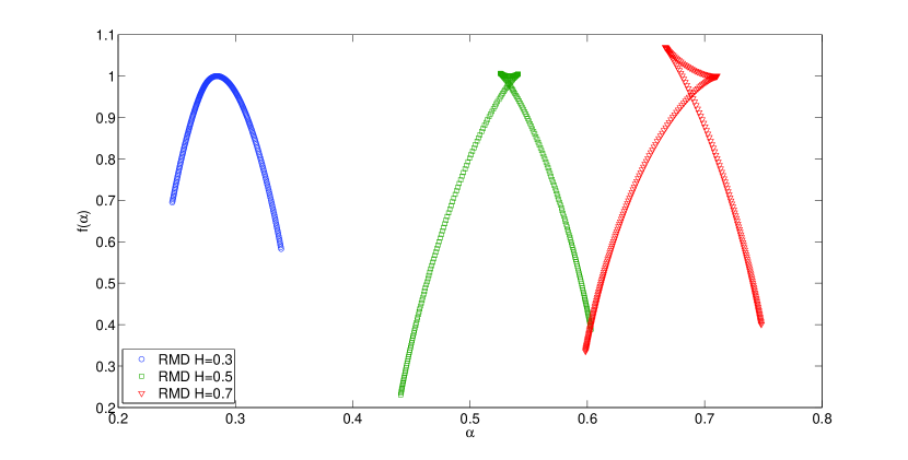
The latter approach makes a useful representation of multifractality. The singularity spectrum in this case should have rather regular form of inverse parabolic shape as shown in Fig.2. The width of spectrum measures the multifractality level of the signal. For the pure monofractal signal this width converges to one point and , while if the bigger amount of multifractality is present in the signal, the width of spectrum becomes wider.
We will analyze in this paper multifractal properties of real financial time series using representation and MF-DFA method argued as working better than other approaches [15]. Our main task is to investigate how multifractal properties of stocks change with variety of ”surgeries” done on the initial real financial time series. We shall do this in following chapters. Our aim is to see what phenomena on the market influence its multifractal dynamics in the first place. In particular, we will focus on examining how multifractal picture of real time series is changed when one cuts off extreme events like crashes or rupture points, and how established trends or their absence influence the multifractal behavior of developed and developing markets.
2 Multifractal noise in monofractal signal of finite length
All statistical methods determining the fractal properties of time series give an exact result only for series of infinite length. Since this applies also to the MF-DFA scheme, one should know how the length of series is an important factor in discovering its multifractal structure. In fact, finite signals assumed by their construction to be monofractals, reveal some artificial multifractal structure. This is because big fluctuations in finite time series, measured within MF-DFA, seem to be more rare than for longer or infinite time series. It leads to smaller value for in finite series than for infinite ones, and finally, to some artificial multifractal structure of finite time series. This kind of multifractal noise should be subtracted first as a background influencing any real property of monofractal or multifractal time series of finite length.
To explore this issue we must have a ”test series“ with known fractal characteristic. We will use monofractal series generated by the random midpoint displacement (RMD) algorithm [22].
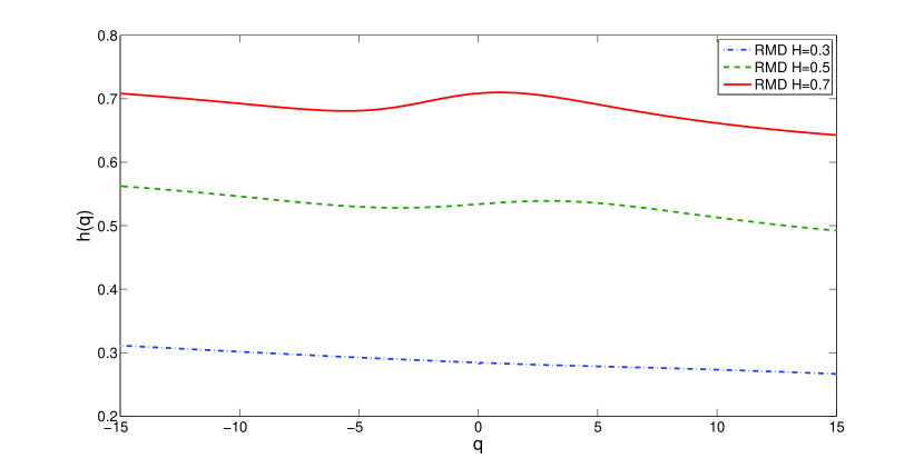
The resulting h(q) functions calculated within MF-DFA for three series of length generated with input Hurst exponent values respectively are presented in Fig. 1.
One may notice a small degree of multifractality (short span of ) for all three series. The series with higher show a bigger deviation from monofractality.
The non-monotonic behaviour of is reflected by the ”twist“ on top of the singularity spectrum (see Fig. 2). This effect will be also observed in following chapters where real financial data are analyzed.
One can also see that the maxima positions of the spectra reflect the assumed Hurst exponents values.
It is essential to find the influence of series length on the width of multifractal spectrum. To observe this, one has to calculate the highest and lowest value of , as well as the position of the peak. This was done on a sample of 20 series each for four lengths and for different values. The width of spectrum was rapidly changing with and seemed to be weakly dependent on . Table 1 presents results found for .
| Series length | Spectrum width | Peak position |
| 0.73 | 0.56 | |
| 0.28 | 0.50 | |
| 0.21 | 0.50 | |
| 0.22 | 0.51 |
They confirm the significant narrowing of spectrum width when the length of time series is increasing. Since we will deal later on with series lengths around , we may assume that the finite size effects should be around .
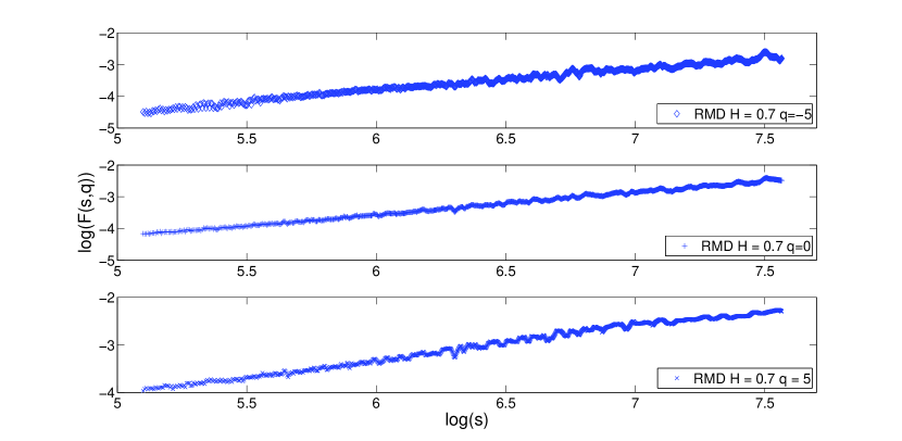
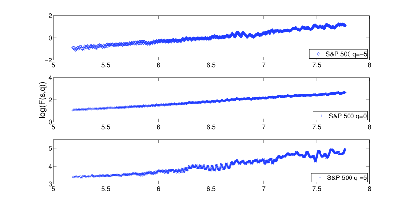
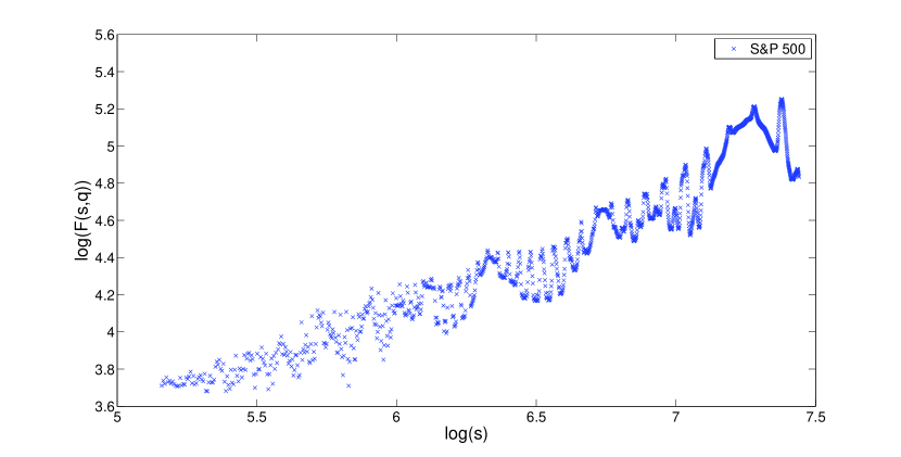
Before analyzing real data we also need to observe the scaling range of the relation. For the artificial data, this range spans almost the entire available time window lengths (see Fig. 3). However, for the entire set of real data (later sections will also discuss parts of these data), the scaling range becomes shorter and decreases with increasing values.
The corresponding effect for the S&P500 is visible in Fig. 4. It is even more significant for positive and larger what is shown in Fig. 5 (compare with Fig. 4). To solve this problem a careful separate study of all relations and manual selection of the scaling range is needed. It was done in analysis of all financial data presented below.
3 Long-term data analysis
The first and most obvious approach is to make the long-term data analysis, i.e., to calculate the multifractal structure of the stock market indices in the whole available time horizon. Our analysis focuses on two indices:
-
•
WIG (Warsaw Stock Exchange)) - from April 16th 1991 till October 10th 2008
-
•
S&P500 (NYSE & Nasdaq) - from December 30th 1927 till September 3rd 2008
They are examples of developing (Poland) and developed (USA) markets respectively.
All time series were created from daily closing values of each index. The S&P 500 data were downloaded from the financial web-site of Yahoo.com [18] and WIG data from a stock market web-site of Wirtualna Polska [19].
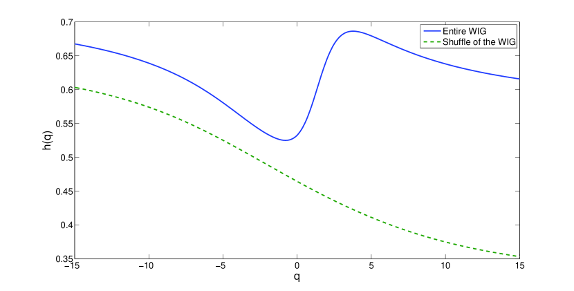
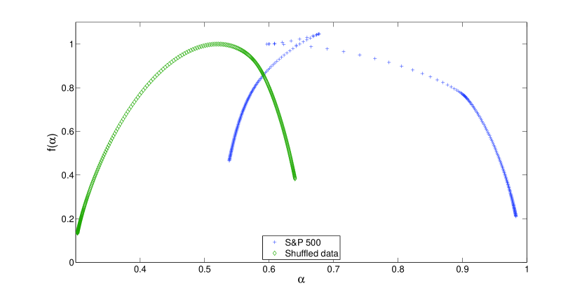
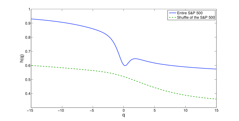
The singularity spectra and plots of all discussed time series (as well as their shuffles) are presented in Figs 6, 7. Surprisingly, all markets show unexpected non-monotonic behavior. This phenomenon, in addition to the problems with short scaling ranges (mentioned in the previous section), strongly suggests a disturbance in the multifractal structure of the series. Spectra of all three shuffled data sets are positioned around the expected location . These sets of data also show a monotonic behavior of the function, contrary to originally ordered data. The spectra width for original as well for shuffled data are much wider than those of the corresponding RMD spectra and hence indicate the multifractal content in dynamics of long-term market data. Simultaneously, the non-monotonic behavior seems to indicate non-stationary effects in these data. The latter case needs more detailed study partly provided below.
4 Multifractal analysis of financial data in established trends
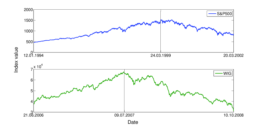
It has been shown by a number of authors (see e.g.[5,20,21]) that positive and negative fluctuations in time series have different fractal properties. Oświȩcimka et. al. has shown in Ref.[5] that DAX data in increasing and decreasing trends has different multifractal properties for particular choice of periods Dec.1997-Dec.1999 and May 2004-May 2006. It is quite natural to investigate whether these properties are general and if so, in what extent they are general for other markets. In particular, it is interesting to know how multifractal properties of established trends depend on the internal structure of these trends. We were interested in the beginning in positive (negative) long-lasting trends with no sub-trends in opposite direction. We tried to exactly repeat this way the analysis made for DAX in Ref.[5]. Such trends turned out to be very rare for S&P 500 and WIG indices. The selected fragments of both indices with required properties are shown in Fig. 8. They have both long-lasting positive trend (bullish phase) followed by a long negative trend (bearish phase) and no astonishing internal events.
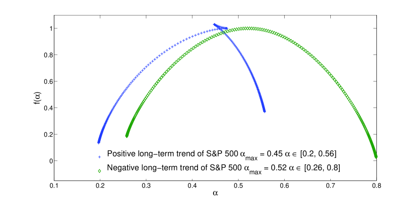
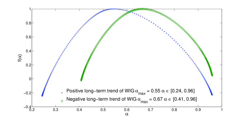
The resulting singularity spectra (see Fig.9) show the expected shift of the bearish phase spectra towards higher values of . Since these results were obtained from data with a much wider scaling range, they should be considered as much more reliable then previous ones presented for entire indices. It is also worth noting that the spectra are now much wider, which suggest a more complex multifractal structure. In the case of WIG this effect might be amplified by the short data set, nevertheless the spectra width of a RMD series with similar length is still narrower.
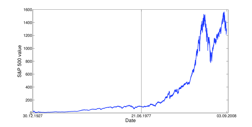
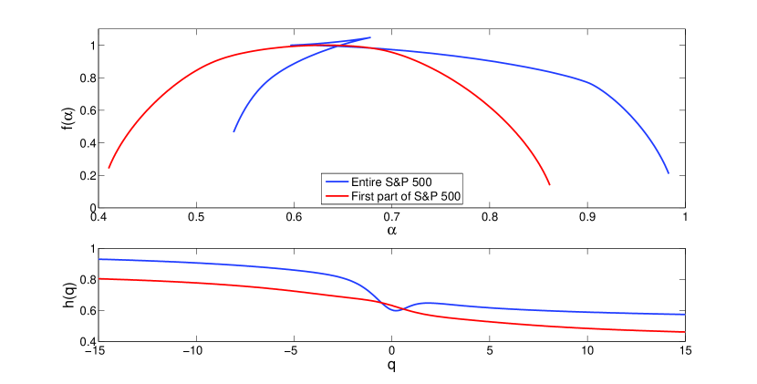
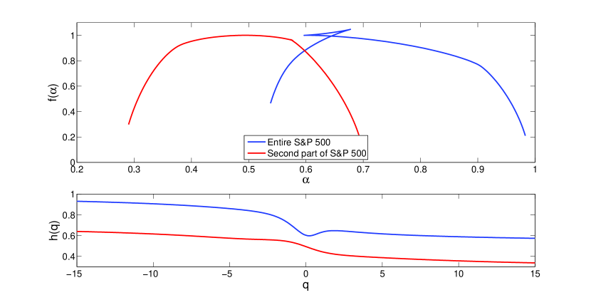
This improvement of singularity spectra for well determined trends in both indices (i.e. quasi quadratic dependence from ) with respect to spectra obtained for the entire indices might suggest that the multifractality is strongly affected by non-stationarity of financial time series. To verify such hypothesis we checked what multifractal properties are hidden in subparts of entire index. The S&P500 index is particularly good for this search because it is long enough comparing with WIG, thus containing much more amount of data. If one divides the entire S&P500 history into two regimes - one with small fluctuations (small volatility) and the second one with high fluctuations (high volatility) as shown in Fig. 10, a very intriguing result for singularity spectra is found in both regimes. Results of this search are plotted in Figs.11, 12, where a comparison of singularity spectra and dependence for both regimes with and behavior for the entire index is provided. It is clear that both regimes show separately a monotonic dependence leading to reversed parabolic shape of . It is not the case of the entire index.
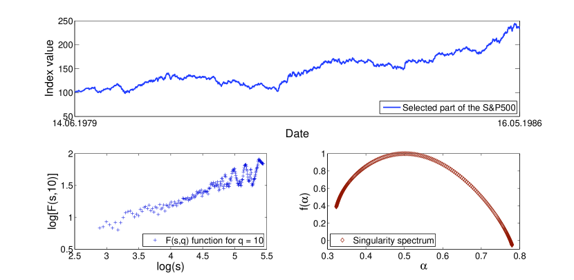
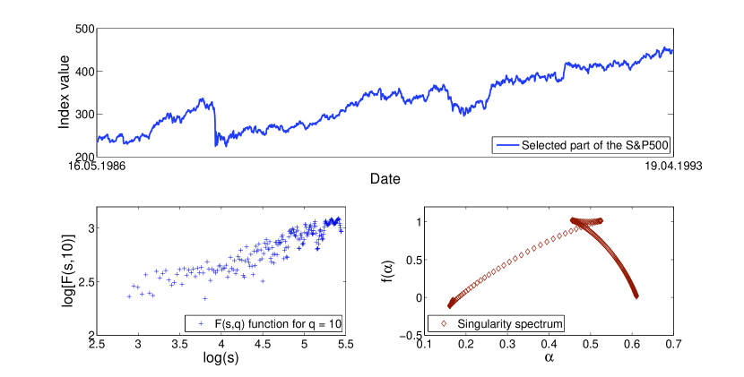
However, both spectra for two regimes are slightly different – the width of multifractal spectrum (and the width of dependence) is larger for the first regime characterized by lower volatility and no opposite sub-trends inside. We checked the same happened for other, even shorter trends, whenever they are affected by well formed sub-trends of opposite direction or by extreme events like crashes, etc. This phenomena is shown on example of S&P500 time series without and with internal structure (see Figs.13, 14). Fig.13 presents an example of increasing trend with no visible distortion inside. We called it ”good” data. Its dynamics is associated with nice multifractal properties - well established quadratic dependence and the monotonic behaviour. Simultaneously, time series of the same length, but collecting data from the very next period, has some extreme events inside and it contains opposite sub-trends connected with these events (see Fig.14). We call them ”bad” data. The scaling is worse here and the presence of ”twist” in singularity spectrum confirms the non-monotonic character of function and leads also to non-quadratic dependence. The multifractal character of time series is here very much affected by the presence of abrupt events, i.e. crashes or data with respectively large fluctuations.
5 Influence of extreme events on multifractal dynamics of stocks
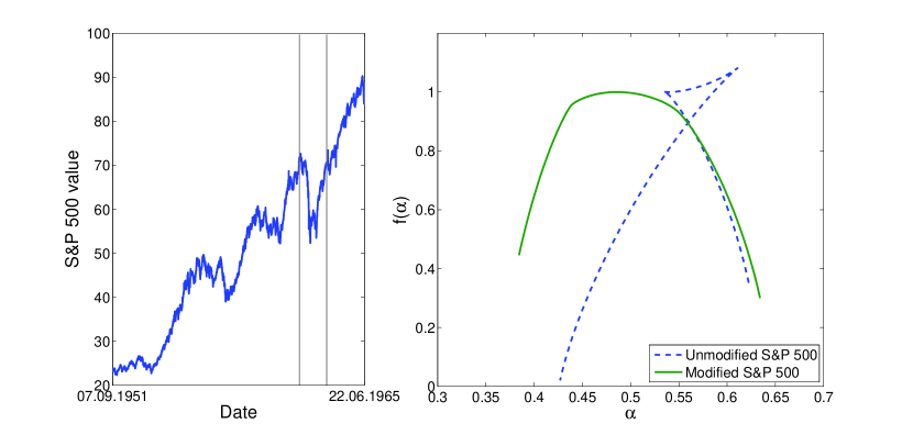
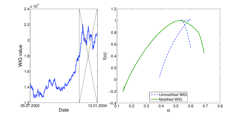
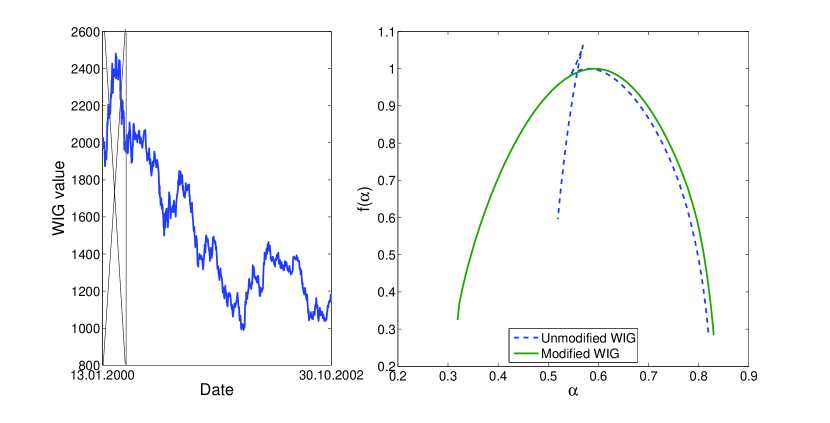
The sub-trends containing abrupt events can be artificially removed to see if such removal would improve the multiscaling properties of the new trend constructed after such ”surgery”. The applied procedure is simple. First, the time series with abrupt events is differentiated. Then, at the level of returns, these events are removed and the time series of remaining returns is integrated to get the new artificial evolution of financial index. Examples of such modification are visible for variety of events for both S&P 500 and WIG indices in Figs.15, 16 and 17 respectively. It is remarkable, how much such surgery significantly improves multi-scaling properties of financial time series and restores the monotonic character of decreasing function. The width of singularity spectrum has also noticeably increased when abrupt events had been removed.
6 Conclusions
We presented a comparative analysis of multifractal properties of financial time series built from stock indices of developing (WIG) and emergent (S&P500) markets using MF-DFA technique. We found that financial time series in a very long time horizon show in both cases very short multiscaling ranges and in turn, their multifractal image is somehow obscured. Therefore we analyzed in shorter time horizon the selected parts of financial data chosen due to their specific properties.
The most important result is that division of time series into regimes of distinctly different (large or small) fluctuations around the main trend, as well as removal of abrupt events like crashes or significant opposite sub-trends, radically improves the multiscaling ranges and restores the monotonic behavior of dependence as well as the reversed parabolic shape of multifractal singularity spectrum . The width of singularity spectrum also increases noticeably in these cases. This leads us to conclusion that non-stationarity of financial time series significantly influences their multifractal character leading to behavior beyond our expectation for multifractal spectrum shape known from studies with artificially created mono- and multifractal signals.
It is clear that further research of length effects as well as the effects of non-stationarity in real time series influencing multiscaling and multifractality is needed with hope for further practical applications.
References
- [1] J.W. Kantelhardt, arXiv: 0804.0747v1 [physics.data-an]
- [2] Z. Eisler, J. Kertész, Physica A 343 (2004) 603
- [3] H.G.E. Hentschel, I. Procaccia, Physica D 8 (1983) 435
- [4] T.C Halsey, M.H. Jensen, L.P. Kadanoff, I. Procaccia, B.I. Shraiman, Phys. Rev. A33 (1983) 1141
- [5] P. Oświȩcimka, J. Kwapień, S. Drożdż, A.Z. Górski, R. Rak, Acta Phys. Pol. A 114 (2008) 547
- [6] J.W. Kantelhardt, E. Koscielny-Bunde, H.H.A. Rego, S. Havlin, A. Bunde, Physica A 295 (2001) 441
- [7] C.-K. Peng, S.V. Buldyrev, S. Havlin, M. Simons, H.E. Stanley, A.L. Golberger, Phys. Rev. E 49 (1994) 1685
- [8] N. Vandewalle, M. Ausloos, Physica A 246 (1997) 454
- [9] M. Ausloos, N. Vandewalle, Ph. Boveroux, A. Minguet, K. Ivanova, Physica A 274 (1999) 229
- [10] G. M. Viswanathan, C.-K. Peng, H.E. Stanley, A.L. Goldberger, Phys. Rev. E 55 (1997) 845
- [11] K. Hu, P. Ch. Ivanov, Z. Chen, P. Carpena, H. E. Stanley, Phys. Rev. E 64 (2001) 011114
- [12] H.E. Hurst, Trans. Am. Soc. Civ. Eng. 116 (1951) 770
- [13] B.B. Mandelbrot, J.R. Wallis, Water Resour. Res. 5(2) (1969) 321
- [14] J.W. Kantelhardt, S.A. Zschiegner, E. Koscielny-Bunde, S. Havlin, A. Bunde, H.E. Stanley, Physica A 316 (2002) 87
- [15] P. Oświȩcimka, J. Kwapień, S. Drożdż, A.Z. Górski, R. Rak, Acta Phys. Pol. B 36 (2005) 2447
- [16] F. Feder, Fractals (Plenum Press, New York 1988)
- [17] H.-O. Peitgen, H. Jürgens, D. Saupe, Chaos and fractal (Springer, Berlin, 2004)
- [18] http://finance.yahoo.com/
- [19] http://gielda.wp.pl/
- [20] K. Ohashi, L.A.N Amaral, B.H. Natelson, Y. Yamamoto, Phys. Rev. E 68 (2003) 065204(R)
- [21] N.B. Ferreira, R. Menezes, D.A. Mendes, Physica A 382 (2007) 73
- [22] R.H. Voss, Random fractal forgeries, in: R.A. Earnshaw (ed.), Fundamental Algorithm for Computer Graphics, NATO ASI Series, Vol. F17, Springer, Berlin, Heidelberg, 1985