arXiv: 0912.3388 [hep-ph]
On Non-Unitary Lepton Mixing and Neutrino Mass Observables

Abstract

There are three observables related to neutrino mass, namely the kinematic mass in direct searches, the effective mass in neutrino-less double beta decay, and the sum of neutrino masses in cosmology. In the limit of exactly degenerate neutrinos there are very simple relations between those observables, and we calculate corrections due to non-zero mass splitting. We discuss how the possible non-unitarity of the lepton mixing matrix may modify these relations and find in particular that corrections due to non-unitarity can exceed the corrections due to mass splitting. We furthermore investigate constraints from neutrino-less double beta decay on mass and mixing parameters of heavy neutrinos in the type I see-saw mechanism. There are constraints from assuming that heavy neutrinos are exchanged, and constraints from assuming light neutrino exchange, which arise from an exact see-saw relation. The latter has its origin in the unitarity violation arising in see-saw scenarios. We illustrate that the limits from the latter approach are much stronger. The drastic impact on inverse neutrino-less double beta decay $(e^{-}e^{-}\rightarrow W^{-}W^{-})$ is studied. We furthermore discuss neutrino mixing in case there is one or more light sterile neutrino. Neutrino oscillation probabilities for long baseline neutrino oscillation experiments are considered, and the analogy to general non-unitarity phenomenology, such as zero-distance effects, is pointed out.

1 Introduction

Even though neutrino mass and lepton mixing are firmly established facts, there is a plethora of open issues still to be addressed. Two of those questions concern the scale of neutrino mass and whether the lepton mixing matrix is unitary. In this letter we would like to discuss in particular some aspects that arise when one combines these two aspects.

The surprisingly large amount of phenomenology of a non-unitarity lepton mixing matrix has recently been discussed by various authors [1, 2, 3, 4, 5, 6, 7, 8, 9, 10]. The observable consequences range from non-standard phenomena in neutrino oscillation experiments [4, 5, 6] to modified properties of leptogenesis [8]. One particular aspect, which so far has only been partly discussed in Refs. [7, 9], is the impact of non-unitarity on observables related to neutrino mass. There are three experimental avenues and measurable quantities to pin down neutrino mass, namely (i) direct searches probing $m_{\beta}$; (ii) neutrino-less double beta decay probing $\langle m\rangle$; (iii) cosmology probing $\Sigma$. In the testable case of quasi-degenerate neutrinos with a mass scale $m_{0}$, and when one neglects the small mass splittings, unitarity of the lepton mixing matrix leads to the relation $\mbox{$\langle m\rangle$}^{\rm max}=m_{\beta}=\Sigma/3$, where $\mbox{$\langle m\rangle$}^{\rm max}$ denotes the maximal value of $\langle m\rangle$. We discuss how non-unitarity of the mixing matrix affects this relation and compare these effects with the inevitable effect of non-zero mass splitting. Surprisingly, the effect of non-unitarity can lead to larger corrections, though the overall effect is small of course.

We furthermore revisit the content of Ref. [7], which uses present limits from neutrino-less double beta decay (0$\nu\beta\beta$) to test mass and mixing parameters of heavy neutrinos in the type I see-saw mechanism. The limits which are obtained when one assumes that light neutrinos are exchanged in the 0$\nu\beta\beta$-diagram can (in the type I see-saw) be exactly related to heavy neutrino parameters. This is possible because the lepton mixing matrix in see-saw scenarios is non-unitary. One can compare these limits with the constraints arising when one assumes that these heavy neutrinos are exchanged in the 0$\nu\beta\beta$-diagram. We illustrate that the limits on the heavy mass and mixing parameters from light neutrino exchange are much stronger than the ones from heavy neutrino exchange. The impact of this approach on inverse neutrino-less double beta decay $(e^{-}e^{-}\rightarrow W^{-}W^{-})$ is also studied, and it is shown that the process is heavily suppressed.

Finally, we discuss the presence of light sterile neutrinos in addition to the three active ones. In this situation the $3\times 3$ matrix which describes the mixing of active neutrinos amongst each other is in general not unitary. We show how to identify the mixing parameters of the sterile neutrinos with the small parameters commonly used to parameterize a non-unitary mixing matrix $N$, namely in $N=(1+\zeta)\,U_{0}$, where $U_{0}$ is unitary and $\zeta$ hermitian. We illustrate how these parameters enter the observables related to neutrino mass. Moreover, we note the analogy of this realization of non-unitarity, which is kinematically easily accessible, to the usually considered one, for which it is assumed that the reason for non-unitarity is beyond kinematic reach. For instance, in case of eV² scale mass-squared differences corresponding to the sterile neutrinos, “zero-distance effects” in neutrino oscillation probabilities arise due to the averaged-out oscillations associated with these mass-squared differences.

The letter is build up as follows: in Section 2 we discuss observables related to neutrino mass and their connection in case the mixing matrix is unitary. In Section 3 we let non-unitary enter the game and discuss how this influences the relations among the mass observables. The particular example of type I see-saw parameters and 0$\nu\beta\beta$ is discussed there as well. Finally, in Section 4 the analogy between light sterile neutrinos and non-unitarity is treated, before we conclude in Section 5.

2 Neutrino Mass Observables

In the charged lepton basis the Pontecorvo-Maki-Nakagawa-Sakata (PMNS) matrix $U$ diagonalizes the neutrino mass matrix $m_{\nu}$ and is parameterized as

$$U=\left(\begin{array}[]{ccc}c_{12}c_{13}&s_{12}c_{13}&s_{13}e^{-i\delta}\\[5.69046pt] -s_{12}c_{23}-c_{12}s_{23}s_{13}e^{i\delta}&c_{12}c_{23}-s_{12}s_{23}s_{13}e^{i\delta}&s_{23}c_{13}\\[5.69046pt] s_{12}s_{23}-c_{12}c_{23}s_{13}e^{i\delta}&-c_{12}s_{23}-s_{12}c_{23}s_{13}e^{i\delta}&c_{23}c_{13}\end{array}\right)P\,.$$ (1)

Here $c_{ij}=\cos\theta_{ij}$, $s_{ij}=\sin\theta_{ij}$ and the Majorana phases are contained in the diagonal matrix $P={\rm diag}(1,\,e^{i\alpha_{2}/2},\,e^{i\alpha_{3}/2})$. The eigenvalues of $m_{\nu}$ are the neutrino masses and there are three complementary observables related to them. The most model-independent one is the kinematic mass as measurable in beta decay experiments:

$$m_{\beta}=\sqrt{\sum|U_{ei}|^{2}\,m_{i}^{2}}\,.$$ (2)

The current limit is 2.3 eV [11] and with the KATRIN experiment a 90 % C.L. limit of $m_{\beta}\leq 0.2$ eV will be possible, while a discovery potential of $5\sigma$ for $m_{\beta}=0.35$ eV exists [12]. Presumably unfair to other experiments, we will denote the observable $m_{\beta}$ in the following as the KATRIN observable.

In contrast to the incoherent sum in Eq. (2), neutrino-less double beta decay (0$\nu\beta\beta$) is sensitive to the coherent sum (the “effective mass”)

$$\mbox{$\langle m\rangle$}=\left|\sum U_{ei}^{2}\,m_{i}\right|.$$ (3)

The measured limits on the half-life of neutrino-less double beta decay are around $10^{23}$ and $10^{25}$ y, depending on the nucleus [13]. Depending also on the uncertain nuclear matrix elements, upper limits on $\langle m\rangle$ around 0.5 to 1 eV arise if one assumes that light neutrino exchange is responsible for 0$\nu\beta\beta$. The existing limits on the half-lifes will be improved considerably (by two orders of magnitude or more) in the near future by various experiments [13]. The maximal value of the effective mass,

$$\mbox{$\langle m\rangle$}^{\rm max}=\sum\left|U_{ei}\right|^{2}\,m_{i}\,,$$ (4)

is obtained when all Majorana phases are trivial (e.g., zero) and the three now real terms in the sum of Eq. (3) simply add.

Finally, the sum of neutrino masses,

$$\Sigma\equiv\sum m_{i}\,,$$ (5)

can be extracted from cosmological observations and is bounded from above by about 1 eV, depending on the data set, priors and of course the cosmological model [14]. One expects future limits on $\Sigma$ in the 0.1 eV range.

We can easily relate the different observables in the limit of quasi-degenerate neutrinos. If all mass splittings are set to zero, and the common neutrino mass is denoted with $m_{0}$, then the relation

$$m_{0}=m_{\beta}=\mbox{$\langle m\rangle$}^{\rm max}=\Sigma/3$$ (6)

is immediately obtained when unitarity of $U$ is assumed. Mismatch of these relations would for quasi-degenerate neutrinos indicate that some form of new physics is present, see e.g., [16]. It is known that there are corrections to relations (6) when non-zero mass splitting is taken into account [17].

We will evaluate these corrections in the following: our convention is such that $m_{0}$ is always the heaviest neutrino mass. Hence, in the normal ordering we denote $m_{0}=m_{3}$, while for the inverted ordering $m_{0}=m_{2}$. Defining the quantities

$$\eta_{\odot}=\frac{\mbox{$\Delta m^{2}_{\odot}$}}{2\,m_{0}^{2}}~{}\mbox{ and }~{}\eta_{\rm A}=\frac{\mbox{$\Delta m^{2}_{\rm A}$}}{2\,m_{0}^{2}}\,,$$ (7)

we can obtain the following expressions for the masses

$$\begin{array}[]{cccc}\mbox{normal:}&m_{3}=m_{0}~{},&m_{2}\simeq m_{0}\left(1-\eta_{\rm A}-\frac{1}{2}\,\eta_{\rm A}^{2}\right)~{},&m_{1}\simeq m_{0}\left(1-\eta_{\rm A}-\frac{1}{2}\,\eta_{\rm A}^{2}-\eta_{\odot}\right)\,,\\ \mbox{inverted:}&m_{2}=m_{0}~{},&m_{1}\simeq m_{0}\left(1-\eta_{\odot}\right)~{},&m_{3}\simeq m_{0}\left(1+\eta_{\rm A}-\frac{1}{2}\,\eta_{\rm A}^{2}-\eta_{\odot}\right).\end{array}$$ (8)

We have kept here second order terms for the ratio $\eta_{\rm A}$ of the atmospheric mass-squared difference and $m_{0}^{2}$, which can be of the same order of magnitude as the terms $\eta_{\odot}$ of order solar mass-squared difference divided by $m_{0}^{2}$. This form of expansion will be applied for most of this work, and we mention here already that we will later neglect also terms of order $\eta_{\rm A}^{2}\,|U_{e3}|^{2}$, because they correspond in magnitude to terms of order $\eta_{\odot}^{2}$. With this expansion, the results for the three observables are (we start with assuming a normal mass ordering)

$$\begin{array}[]{c}\displaystyle m_{\beta}\simeq m_{0}\left(1-c_{13}^{2}\,\eta_{\rm A}-\frac{1}{2}\,c_{13}^{4}\,\eta_{\rm A}^{2}-c_{12}^{2}\,c_{13}^{2}\,\eta_{\odot}\right)\equiv\tilde{m}_{\beta}\,,\\ \displaystyle\mbox{$\langle m\rangle$}^{\rm max}\simeq m_{\beta},\\ \displaystyle\Sigma\simeq 3\,m_{0}\left(1-\frac{2}{3}\,\eta_{\rm A}-\frac{1}{3}\,\eta_{\rm A}^{2}-\frac{1}{3}\,\eta_{\odot}\right)\equiv\tilde{\Sigma}\,.\end{array}$$ (9)

We see that the upper limit of the effective mass and the KATRIN observable are to the order given identical. Their difference is by all means tiny, to be more precise:

$$m_{\beta}-\mbox{$\langle m\rangle$}^{\rm max}\simeq m_{0}\left(\frac{1}{4}\,\sin^{2}2\theta_{12}\,\eta_{\odot}^{2}+|U_{e3}|^{2}\,c_{12}^{2}\,\eta_{\odot}\,\eta_{\rm A}+\frac{1}{2}\,|U_{e3}|^{2}\,\eta_{\rm A}^{2}\right)\equiv m_{0}\,\Delta_{1}\,.$$ (10)

Numerically, if we choose $m_{0}=0.3$ eV and insert [15] $\mbox{$\Delta m^{2}_{\rm A}$}=2.39\cdot 10^{-3}$ eV², $\mbox{$\Delta m^{2}_{\odot}$}=7.67\cdot 10^{-5}$ eV² and $\sin^{2}\theta_{12}=\frac{1}{3}$, then $\Delta_{1}$ is $2.1\cdot 10^{-8}$ for $U_{e3}=0$ and $3.6\cdot 10^{-6}$ for $|U_{e3}|=0.2$. Any deviation from these numbers will therefore be a clear signal of new physics.

The situation is somewhat different when we consider $\Sigma$. In the fully degenerate regime, we have the relation $\Sigma=3\,m_{\beta}$. Corrections are induced by non-zero splitting, which results in

$$\frac{1}{3}\,\Sigma-m_{\beta}\simeq\frac{1}{3}\,\Sigma-\mbox{$\langle m\rangle$}^{\rm max}\simeq\frac{m_{0}}{6}\left((3\,\cos 2\theta_{13}-1)\,\eta_{\rm A}+\eta_{\rm A}^{2}+(1+3\,\cos 2\theta_{12})\,\eta_{\odot}\right)\equiv m_{0}\,\Delta_{2}\,.$$ (11)

With the same numerical input as above for $\Delta_{1}$, the range of $\Delta_{2}$ is between 0.0046 for $|U_{e3}|=0$ and 0.0041 for $|U_{e3}|=0.2$.

In the inverted ordering, the formulae are basically identical and in particular the size of $m_{\beta}-\mbox{$\langle m\rangle$}^{\rm max}$, as well as of $\frac{1}{3}\,\Sigma-m_{\beta}$ is identical to the normal ordering, except for a sign change for the latter.

3 Non-Unitarity and Neutrino Mass Observables

3.1 General Case

Now let us switch on non-unitarity, or rather switch off unitarity. It proves convenient to write in the relation $\nu_{\alpha}=N_{\alpha i}\,\nu_{i}$, which connects flavor and mass states, the now non-unitary matrix $N$ as [4]

$$N=(1+\eta)\,U_{0}\,,$$ (12)

where $\eta$ is hermitian (containing 6 real moduli and 3 phases because $\eta_{\alpha\beta}=|\eta_{\alpha\beta}|\,e^{i\phi_{\alpha\beta}}$ for $\alpha\neq\beta$) and $U_{0}$ is unitary (containing 3 real moduli and 3 phases). Several observables [3] such as limits on rare lepton decays and universality lead to the following 90% C.L. bounds on the elements of $\eta$:

$$|\eta|=\left(\begin{array}[]{ccc}|\eta_{ee}|&|\eta_{e\mu}|&|\eta_{e\tau}|\\ \cdot&|\eta_{\mu\mu}|&|\eta_{\mu\mu}|\\ \cdot&\cdot&|\eta_{\mu\tau}|\end{array}\right)\leq\left(\begin{array}[]{ccc}2.0\times 10^{-3}&5.9\times 10^{-5}&1.6\times 10^{-3}\\ \cdot&8.2\times 10^{-3}&1.0\times 10^{-3}\\ \cdot&\cdot&2.6\times 10^{-3}\end{array}\right).$$ (13)

These bounds apply to sources of non-unitarity corresponding to energies much larger than experimentally accessible. Mixing of light neutrinos with heavy (say, with masses $\mathrel{\hbox to0.0pt{\raise 2.20013pt\hbox{$>$}\hss}{\lower 2.20013pt\hbox{$\sim$}}}$ TeV) particles is one example for such a situation. Using now $N$ instead of $U$, we can re-evaluate the results from the last Section, in particular the difference of the KATRIN observable $m_{\beta}$ and the maximal value of the effective mass for a normal mass ordering. We find that the parameter $\eta_{ee}$ related to non-unitarity contributes in first order:

$$\begin{array}[]{c}m_{\beta}\simeq\tilde{m}_{\beta}+m_{0}\,|\eta_{ee}|\\ \mbox{$\langle m\rangle$}^{\rm max}\simeq\tilde{m}_{\beta}+2\,m_{0}\,|\eta_{ee}|\,.\end{array}$$ (14)

The term $\tilde{m}_{\beta}$ has been defined above in Eq. (9). The terms $\eta_{e\mu}$ and $\eta_{e\tau}$ contribute only quadratically, the other entries of $\eta$ do not show up at all. Hence, the difference between the effective mass and the KATRIN observable is

$$m_{\beta}-\mbox{$\langle m\rangle$}^{\rm max}\simeq m_{0}\,(\Delta_{1}-|\eta_{ee}|)\,,$$ (15)

where $\Delta_{1}$ is defined in Eq. (10). Applying our example of $m_{0}=0.3$ eV, we find that the term $m_{0}\,|\eta_{ee}|$ can be as large as $6.0\cdot 10^{-4}$ eV, which has to be compared with $m_{0}\,\Delta_{1}$ being mostly of order $10^{-6}$ eV. Though the correction from $|\eta_{ee}|$ is below current experimental sensitivities, it is surprising and noteworthy that it can be almost 3 orders of magnitude larger than the correction from mass splitting.

The sum of masses does not depend on the mixing matrix and is therefore not affected by its non-unitarity. For the differences of $\Sigma$ with the KATRIN observable and the maximal effective mass one finds

$$\begin{array}[]{c}\displaystyle\frac{1}{3}\,\Sigma-m_{\beta}\simeq m_{0}\,(\Delta_{2}-|\eta_{ee}|)\,,\\ \displaystyle\frac{1}{3}\,\Sigma-\mbox{$\langle m\rangle$}^{\rm max}\simeq m_{0}\,(\Delta_{2}-2\,|\eta_{ee}|)\,.\end{array}$$ (16)

With our example values discussed above $\Delta_{2}$ is smaller than 0.0046 and thus we see (after recalling that $|\eta_{ee}|<0.0020$) that also the relations $\Sigma/3=m_{\beta}$ and $\Sigma/3=\mbox{$\langle m\rangle$}^{\rm max}$ can be modified by non-unitarity to a larger extent than due to mass-splitting.

In the inverted ordering one finds the same corrections to the differences of observables than for the normal ordering.

3.2 Heavy Neutrino Mixing in the type I See-Saw

Within the conventional type I see-saw there is a guaranteed source of unitarity violation, namely the inherent mixing of the light neutrino states with the heavy ones. The complete mass term containing the Dirac and Majorana masses can be written as

$${\cal L}=\overline{\nu_{L}}\,m_{D}\,N_{R}+\frac{1}{2}\,\overline{N_{R}^{c}}\,M_{R}\,N_{R}+h.c.=\frac{1}{2}\,(\overline{\nu_{L}},\overline{N_{R}^{c}})\left(\begin{array}[]{cc}0&m_{D}\\ m_{D}^{T}&M_{R}\end{array}\right)\left(\begin{array}[]{c}\nu_{L}^{c}\\ N_{R}\end{array}\right)+h.c.,$$ (17)

and it is diagonalized by a unitary $6\times 6$ matrix

$${\cal U}=\left(\begin{array}[]{cc}N&S\\ T&V\end{array}\right)\mbox{ with }{\cal M}={\cal U}\left(\begin{array}[]{cc}m_{\nu}^{\rm diag}&0\\ 0&M_{R}^{\rm diag}\end{array}\right){\cal U}^{T}\,.$$ (18)

Since the eigenvalues of $M_{R}$ are much bigger than the elements of $m_{D}$, the entries of $S$ and $T$ are of order $m_{D}/M_{R}$, and hence one can obtain the expression

$$-N^{\dagger}\,m_{D}\,M_{R}^{-1}\,m_{D}^{T}\,N^{\ast}=m_{\nu}^{\rm diag}\,.$$ (19)

The matrix $S$ characterizes the mixing of the light neutrinos with the heavy ones:

$$\nu_{\alpha}=N_{\alpha i}\,\nu_{i}+S_{\alpha i}\,N_{i}\,,$$ (20)

where $\nu_{i}$ ($N_{i}$) are the light (heavy) neutrinos with $i=1,2,3$ and $\alpha=e,\mu,\tau$. Therefore, the mixing matrix in type I see-saw scenarios is strictly speaking not unitary, since $NN^{\dagger}=\mathbbm{1}-SS^{\dagger}\neq\mathbbm{1}$.

The effective mass in neutrino-less double beta decay is given by

$$\mbox{$\langle m\rangle$}=\left|\sum N_{ei}^{2}\,m_{i}\right|\leq\xi~{}{\rm eV}\,,$$ (21)

and has, as discussed above, a current limit of around 1 eV, depending on the uncertain nuclear matrix elements. We have written therefore the limit as $\xi$ eV, with $\xi={\cal O}(1)$.

To connect the effective mass with the heavy neutrino parameters, one notes that the 11-element of Eq. (18) reads $N\,m_{\nu}^{\rm diag}\,N^{T}+S\,M_{R}^{\rm diag}\,S^{T}=0$. Therefore, for the effective mass holds [7]

$$\left|\sum N_{ei}^{2}\,m_{i}\right|=\left|\sum S_{ei}^{2}\,M_{i}\right|\,.$$ (22)

Consequently, the experimental limits on $\langle m\rangle$ apply directly to this combination of parameters:

$$\left|\sum S_{ei}^{2}\,M_{i}\right|\leq\xi~{}\rm eV\,.$$ (23)

This relation has been discussed first in Ref. [7], and here we illustrate its phenomenological consequences further. Note that this relation has its origin in the necessary unitary violation of the PMNS matrix in type I see-saw scenarios. The combination of parameters in Eq. (23) has to be compared with another combination of mass and mixing parameters, which can be constrained from 0$\nu\beta\beta$ [18]:

$$\mbox{$\displaystyle\left\langle\frac{1}{m}\right\rangle$}=\left|\sum S_{ei}^{2}\,\frac{1}{M_{i}}\right|\leq\tilde{\xi}~{}5\cdot 10^{-8}\,{\rm GeV}^{-1}\,.$$ (24)

This limit (we have introduced a factor $\tilde{\xi}$ taking into account possible nuclear matrix element uncertainties) is obtained when 0$\nu\beta\beta$ is assumed to be mediated by heavy neutrinos. The origin of the difference between $\langle m\rangle$ and $\displaystyle\left\langle\frac{1}{m}\right\rangle$ is nothing but the two extreme limits of the fermion propagator of the Majorana neutrinos, which is central to the Feynman diagram of 0$\nu\beta\beta$:

$$\frac{{/q}+m_{i}}{q^{2}-m_{i}^{2}}\propto\left\{\begin{array}[]{cc}m_{i}&\mbox{ for }q^{2}\gg m_{i}^{2}\\ \frac{\displaystyle 1}{\displaystyle m_{i}}&\mbox{ for }q^{2}\ll m_{i}^{2}\end{array}\right.\,.$$ (25)

Here $q$ denotes the momentum transfer in the process under study, which is around $10$ to $100$ MeV, corresponding to $1/r$, where $r\simeq 10^{-12}$ cm is the average distance of the two decaying nuclei.

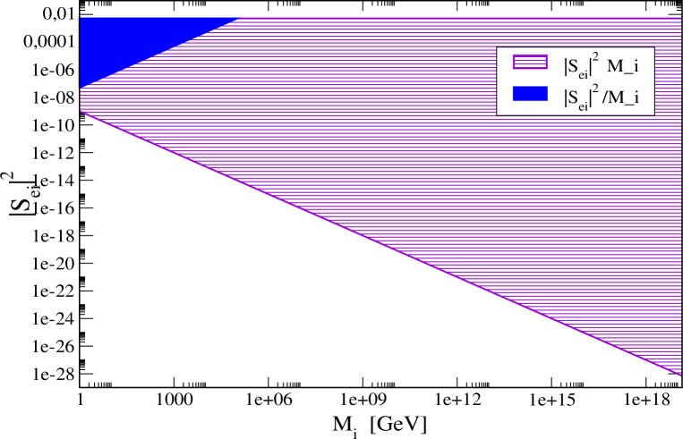
Figure 1: Constraints on heavy Majorana neutrino parameters from neutrino-less double beta decay. The horizontally striped (violet) area is forbidden by $|S_{ei}|^{2}\,M_{i}<1$ eV, while the filled (blue) area is forbidden by $|S_{ei}|^{2}/M_{i}<5\cdot 10^{-8}$ GeV^-1. The general upper limit is $|S_{ei}|^{2}<0.0052$.

We see that $\langle m\rangle$ and $\displaystyle\left\langle\frac{1}{m}\right\rangle$ depend on two different combinations of the mass and mixing parameters of the heavy neutrinos. It is a useful exercise to compare the two approaches. Fig. 1 shows the two limits. In what regards the mixing parameter $S_{ei}$, there is an upper limit of [21]

$$|S_{ei}|^{2}\leq 0.0052\,,$$ (26)

obtained from global fits, in particular of LEP data. The horizontally striped (violet) area in Fig. 1 is obtained from $|S_{ei}|^{2}\,M_{i}<1$ eV, while the filled (blue) area is from $|S_{ei}|^{2}/M_{i}<5\cdot 10^{-8}$ GeV^-1. It is clear to see that the constraints from $|S_{ei}|^{2}\,M_{i}<1$ eV are much stronger.

We should note that the limits from $|S_{ei}|^{2}\,M_{i}$ apply to heavy neutrinos of the see-saw mechanism, while limits from $|S_{ei}|^{2}/M_{i}$ apply to any heavy neutral Majorana fermion which mixes with the light fermions. We have also assumed that there is only one heavy neutrino contributing to the sum, and therefore do not take the possibility of fine-tuned cancellations of different terms in the sum into account. We also do not take into account fine-tuned cancellations in neutrino-less double beta decay, i.e., there could be diagrams (e.g. right-handed currents, supersymmetry,$\ldots$) contributing to 0$\nu\beta\beta$, which interfere destructively with the neutrino mass contribution(s).

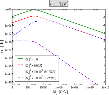
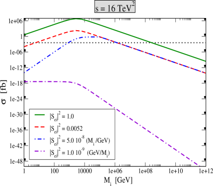
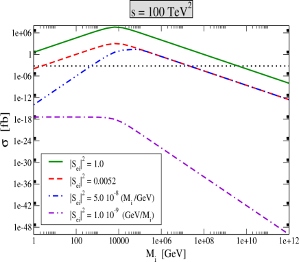
Figure 2: Cross section for $e^{-}e^{-}\rightarrow W^{-}W^{-}$ with $\sqrt{s}=1$ TeV (upper left), $\sqrt{s}=4$ TeV (upper right), $\sqrt{s}=10$ TeV (bottom) and several limits for the mixing parameter $|S_{ei}|^{2}$. The dotted line corresponds to five events for an assumed luminosity of 80 $(s/{\rm TeV^{2}})$ fb^-1.

With these caveats in mind, we continue with studying a frequently considered process related to collider phenomenology of heavy Majorana neutrinos. There are many possibilities for this, but here we focus for simplicity on “inverse neutrino-less double beta decay” [22, 23],

$$e^{-}e^{-}\rightarrow W^{-}W^{-}\,,$$

which may be searched for at future linear colliders in an electron-electron mode. The differential cross section in the limit of negligible mass of the $W^{-}$ and one heavy neutrino $M_{i}$ is

$$\frac{d\sigma}{d\cos\theta}=\frac{G_{F}^{2}}{32\,\pi}\left\{M_{i}\,|S_{ei}|^{2}\left(\frac{t}{t-M_{i}^{2}}+\frac{u}{u-M_{i}^{2}}\right)\right\}^{2}\,.$$ (27)

Evaluating the full cross section for $\sqrt{s}=1$ TeV, 4 TeV, and 10 TeV results in Fig. 2, where we give $\sigma$ for different values of $|S_{ei}|^{2}$. We have also indicated where to expect five events when a luminosity of 80 $(s/{\rm TeV^{2}})$ fb^-1 [23] is achieved. Note that the extreme limits of the cross section, which are given as

$$\sigma=\left\{\begin{array}[]{cc}\displaystyle\frac{G_{F}^{2}}{4\,\pi}\,\left(|S_{ei}|^{2}\,M_{i}\right)^{2}&\mbox{for }s\gg M_{i}^{2}\,,\\ \displaystyle\frac{G_{F}^{2}}{16\,\pi}s^{2}\left(\frac{|S_{ei}|^{2}}{M_{i}}\right)^{2}&\mbox{for }s\ll M_{i}^{2}\,,\end{array}\right.$$ (28)

do not depend on $s$ for negligible masses and are proportional to $s^{2}$ for heavy masses.

The effect of the strong limit $|S_{ei}|^{2}\,M_{i}<1$ eV is again clearly seen. In case of $\sqrt{s}=1$ TeV even the weaker limit (24) from 0$\nu\beta\beta$ renders the process unobservable. For the larger values of $\sqrt{s}=4$ and 10 TeV a large range of values of $M_{i}$ could potentially be probed. However, switching on the limit (23) from the see-saw relation makes the cross section miniscule. This straightforward example shows that the limit (23) makes it much harder to observe any effect of Majorana neutrinos at colliders (if they are see-saw based and no cancellations take place).

4 Light sterile Neutrinos and Non-Unitarity

Another straightforward source of non-unitarity of the $3\times 3$ lepton mixing matrix is the presence of light sterile neutrinos, with masses in the eV regime. We wish to remark in this note a nice analogy between the effects of sterile neutrinos and of kinematically unaccessible non-unitarity, which takes place when neutrino oscillations are considered.

Assuming first the presence of only one sterile neutrino, the total light neutrino mass matrix is now a $4\times 4$ object, and diagonalized by a unitary $4\times 4$ matrix

$$U=\left(\begin{array}[]{cccc}\lx@intercol\hfil\mbox{$N_{3\times 3}$}\hfil\lx@intercol&U_{e4}\\ U_{s1}&U_{s2}&U_{s3}&U_{s4}\end{array}\right).$$ (29)

The “active” $3\times 3$ part $N$, which describes the mixing of $\nu_{e}$, $\nu_{\mu}$ and $\nu_{\tau}$, is not unitarity, because $NN^{\dagger}\neq\mathbbm{1}_{3}$. We parameterize the full $4\times 4$ mixing matrix as

$$U=\tilde{R}_{14}\,R_{24}\,\tilde{R}_{34}\,R_{23}\,\tilde{R}_{13}\,R_{12}\,P\,,$$ (30)

where $P={\rm diag}(1,e^{i\alpha_{2}/2},e^{i\alpha_{3}/2},e^{i\alpha_{4}/2})$ contains the Majorana phases and $R_{ij}$ are rotations around the $ij$-axis, e.g.,

$$R_{23}=\left(\begin{array}[]{cccc}1&0&0&0\\ 0&c_{23}&s_{23}&0\\ 0&-s_{23}&c_{23}&0\\ 0&0&0&1\end{array}\right),~{}~{}\tilde{R}_{14}=\left(\begin{array}[]{cccc}c_{14}&0&0&s_{14}\,e^{-i\delta_{14}}\\ 0&1&0&0\\ 0&0&1&0\\ -s_{14}\,e^{i\delta_{14}}&0&0&1\end{array}\right).$$ (31)

The upper left $3\times 3$ submatrix of $U$ is called $N$. Recall that one can write $N=(1+\zeta)\,U_{0}$ with unitary $U_{0}$ and hermitian $\zeta$, and hence we can identify $2\,\zeta\simeq NN^{\dagger}-\mathbbm{1}$. Expanding in terms of the small mixing angles $\theta_{i4}$, we find from Eq. (30):

$$\zeta\simeq-\frac{1}{2}\left(\begin{array}[]{ccc}\theta_{14}^{2}&\theta_{14}\,\theta_{24}\,e^{-i\delta_{14}}&\theta_{14}\,\theta_{34}\,e^{i(\delta_{34}-\delta_{14})}\\ \theta_{14}\,\theta_{24}\,e^{i\delta_{14}}&\theta_{24}^{2}&\theta_{24}\,\theta_{34}\,e^{i\delta_{34}}\\ \theta_{14}\,\theta_{34}\,e^{-i(\delta_{34}-\delta_{14})}&\theta_{24}\,\theta_{34}\,e^{-i\delta_{34}}&\theta_{34}^{2}\end{array}\right).$$ (32)

We should stress here that the limits on $\eta$ quoted in Eq. (7) do of course not apply to the elements of $\zeta$. The limits on $\eta$ are valid for particles which are kinematically far from being accessible. We note that if the LSND result [24] is analyzed in terms of neutrino oscillations, the angles $\theta_{i4}$ are of order $0.1$. However, in terms of oscillation experiments there are similar effects from sterile neutrinos and from a non-unitary mixing matrix, as we will note in the following.

To illustrate this, consider that the sterile neutrinos have typically mass-squared differences of order eV², i.e., much larger than the solar and atmospheric mass-squared difference. It suffices to make our point for the simple case of a high-energy, short-baseline neutrino factory with baseline $L=130$ km (CERN–Frejus) and a muon energy of $E_{\mu}=50$ GeV. One can neglect matter effects and the solar neutrino mass-squared difference, hence set $\mbox{$\Delta m^{2}_{\odot}$}=m_{2}^{2}-m_{1}^{2}$ to zero, while the oscillations corresponding to $\Delta m^{2}_{41}\simeq\Delta m^{2}_{42}\simeq\Delta m^{2}_{43}\simeq$ eV² average out. The oscillation probability is in general

$$P_{\alpha\beta}=\left|\sum_{j}U_{\beta j}\,U_{\alpha j}^{\ast}\,e^{-im_{j}^{2}L/(2E)}\right|^{2},$$ (33)

and for the case of one sterile neutrino the sum goes from 1 to 4. For muon to tau neutrinos the probability is given by

$$\begin{array}[]{c}\displaystyle P(\nu_{\mu}\rightarrow\nu_{\tau})^{\rm St}\simeq\sin^{2}2\theta_{23}\,(1-2\,|U_{e3}|^{2})\,\sin^{2}\frac{\Delta_{13}}{2}+\theta_{24}\,\theta_{34}\,\sin\delta_{34}\,\sin\Delta_{13}\\ \displaystyle-(\theta_{24}^{2}+\theta_{34}^{2})\,\sin^{2}2\theta_{23}\,\sin^{2}\frac{\Delta_{13}}{2}+\ldots+2\,\theta_{24}^{2}\,\theta_{34}^{2}\,.\end{array}$$ (34)

We have expanded the lengthy result in terms of the small parameters $|U_{e3}|$ and $\theta_{i4}$, and $\Delta_{31}=(m_{3}^{2}-m_{1}^{2})\,L/(2E)$ corresponds to the oscillations of the atmospheric mass-squared difference. The second term in Eq. (34) is an “interference term” of the sterile neutrino mixing parameter with the leading oscillations. From the many higher order terms we have given here only the constant one, which is particularly interesting. Namely, it introduces a constant contribution stemming purely from the averaged-out sterile neutrino mass-squared difference. This resembles the “zero-distance” effect in case of a non-unitary mixing matrix [1], which denotes a constant non-zero transition probability also in the limit of zero baseline. To further study this, consider the neutrino oscillation probability for a non-unitary PMNS matrix and its zero baseline limit:

$$P^{\rm NU}(\nu_{\alpha}\rightarrow\nu_{\beta})=\frac{\left|\sum_{j}N_{\beta j}\,N_{\alpha j}^{\ast}\,e^{-im_{j}^{2}L/(2E)}\right|^{2}}{(NN^{\dagger})_{\alpha\alpha}\,(NN^{\dagger})_{\beta\beta}}\stackrel{{\scriptstyle L\rightarrow 0}}{{=}}\frac{\left|(NN^{\dagger})_{\beta\alpha}\right|}{(NN^{\dagger})_{\alpha\alpha}\,(NN^{\dagger})_{\beta\beta}}\,.$$ (35)

To be more specific, for the same experimental setup as before, and for the muon to tau channel one finds after an expansion to second order in $|U_{e3}|$ and $\eta_{\mu\tau}$:

$$\begin{array}[]{c}\displaystyle P(\nu_{\mu}\rightarrow\nu_{\tau})^{\rm NU}\simeq(1-2\,|U_{e3}|^{2})\,\sin^{2}2\theta_{23}\,\sin^{2}\frac{\Delta_{31}}{2}-2\,|\eta_{\mu\tau}|\,\sin 2\phi_{\mu\tau}\,\sin 2\theta_{23}\,\sin\Delta_{31}\\ \displaystyle+|\eta_{\mu\tau}|^{2}\left(4-2\,(3-\cos\phi_{\mu\tau})\,\sin^{2}\frac{\Delta_{31}}{2}\right).\end{array}$$ (36)

We have kept only $\eta_{\mu\tau}$ in the above expression, because it is the leading non-unitarity parameter in $P(\nu_{\mu}\rightarrow\nu_{\tau})^{\rm NU}$ [4, 5]. In analogy to the expression (34) for sterile neutrino oscillations, the second term of order $|\eta_{\mu\tau}|$ is an interference term with the oscillations, while the third term of order $|\eta_{\mu\tau}|^{2}$ gives rise to a constant contribution: the zero distance effect. Indeed, in the limit of vanishing baseline:

$$P(\nu_{\mu}\rightarrow\nu_{\tau})^{\rm NU}\stackrel{{\scriptstyle L\rightarrow 0}}{{\simeq}}4\,|\eta_{\mu\tau}|^{2}\,.$$ (37)

The structure of the two oscillation probabilities is identical, and governed (up to a factor 2) by the same element of $\zeta$ and $\eta$, respectively (note that $\theta_{24}^{2}\,\theta_{34}^{2}=4\,|\zeta_{\mu\tau}|^{2}$). While for the sterile neutrino case the constant term arises due to the averaged-out oscillation term of the large $\Delta m^{2}$, for non-unitarity the non-orthogonality of the neutrino states is the reason.

The same analysis can be performed for the maybe more motivated case [26] of two additional sterile neutrinos. Parameterizing

$$U=\tilde{R}_{15}\,\tilde{R}_{14}\,\tilde{R}_{35}\,R_{24}\,\tilde{R}_{25}\,\tilde{R}_{34}\,R_{23}\,\tilde{R}_{13}\,R_{12}\,P\,,$$ (38)

one finds in the same way as above

$$\zeta\simeq-\frac{1}{2}\left(\begin{array}[]{ccc}\theta_{14}^{2}+\theta_{15}^{2}&\theta_{14}\,\theta_{24}\,e^{-i\delta_{14}}+\theta_{15}\,\theta_{25}\,e^{i(\delta_{25}-\delta_{15})}&\theta_{14}\,\theta_{34}\,e^{i(\delta_{34}-\delta_{14})}+\theta_{15}\,\theta_{35}\,e^{i(\delta_{35}-\delta_{15})}\\ \cdot&\theta_{24}^{2}+\theta_{25}^{2}&\theta_{24}\,\theta_{34}\,e^{-i\delta_{34}}+\theta_{25}\,\theta_{35}\,e^{i(\delta_{35}-\delta_{25})}\\ \cdot&\cdot&\theta_{34}^{2}+\theta_{35}^{2}\end{array}\right).$$

The off-diagonal terms not written down explicitly are simply the complex conjugates of the terms from the other side of the diagonal. The oscillation probability reads

$$\begin{array}[]{c}\displaystyle P(\nu_{\mu}\rightarrow\nu_{\tau})^{\rm St}\simeq\sin^{2}2\theta_{23}\,(1-2\,|U_{e3}|^{2})\,\sin^{2}\frac{\Delta_{13}}{2}\\ \displaystyle+\left(\theta_{24}\,\theta_{34}\,\sin\delta_{34}+\theta_{25}\,\theta_{35}\,\sin(\delta_{35}-\delta_{25})\right)\sin\Delta_{13}\\ \displaystyle-\left(\theta_{24}^{2}+\theta_{34}^{2}+\theta_{25}^{2}+\theta_{35}^{2}\right)\sin^{2}2\theta_{23}\sin^{2}\frac{\Delta_{13}}{2}\,,\end{array}$$ (39)

and is governed by the entries $\zeta_{\mu\mu}$, $\zeta_{\mu\tau}$ and $\zeta_{\tau\tau}$. In analogy to the case of one sterile neutrino, there is a constant “zero distance contribution” coming from the fourth order terms, which read $2\left(\theta_{24}^{2}\,\theta_{34}^{2}+\theta_{25}^{2}\,\theta_{35}^{2}\right)$.

We conclude that long baseline oscillation probabilities show similar properties for sterile neutrinos with mass-squared differences exceeding roughly 0.1 eV² and for general non-unitarity. Of course, the phenomenology in other sectors, even other oscillation experiments, is very different. In what regards mass-related observables, the eV scale states contribute to the cosmological sum of masses, and also to $m_{\beta}$ and $\langle m\rangle$. For the latter two the relevant expression is

$$U_{e4}^{2}\,m_{4}=m_{4}\,c_{24}^{2}\,c_{34}^{2}\,s_{14}^{2}\,e^{i(\alpha_{4}+2\delta_{14})}\simeq m_{4}\,\theta_{14}^{2}\,e^{i(\alpha_{4}+2\delta_{14})}\simeq m_{4}\,e^{i(\alpha_{4}+2\delta_{14})}\,|\zeta_{ee}|^{2}\,.$$ (40)

If the three active neutrinos are quasi-degenerate, $m_{4}$ needs to be larger than $m_{0}$ (to avoid too many problems with cosmology), such that there will be a large effect for the observables related to neutrino mass. The phenomenology of those scenarios is discussed e.g. in [28].

Also in the case of two additional sterile neutrinos there is interesting mass-related phenomenology, for which we refer to Ref. [29]. The important quantity is

$$U_{e4}^{2}\,m_{4}+U_{e5}^{2}\,m_{5}\simeq\theta_{14}^{2}\,e^{i(\alpha_{4}-2\delta_{14})}\,m_{4}+\theta_{15}^{2}\,e^{i(\alpha_{5}-2\delta_{15})}\,m_{5}\,,$$ (41)

which, unlike the 4 neutrino case, does not correspond directly to an element of $\zeta$, unless there is a hierarchy in the form of $\theta_{14}^{2}\ll\theta_{15}^{2}$ or $\theta_{14}^{2}\gg\theta_{15}^{2}$.

5 Summary and Conclusions

Non-unitarity of the lepton mixing matrix affects the observables relevant to lepton mixing and neutrino mass. Here we noted three possibilities related to this issue. We have first discussed the general case: for quasi-degenerate neutrinos with a common mass scale $m_{0}$, there can be corrections to the naive relations $\mbox{$\langle m\rangle$}^{\rm max}=m_{\beta}=\Sigma/3$, which are larger than the corrections stemming from the non-degeneracy of the masses. Second, in the context of the type I see-saw mechanism, it was discussed before that limits from light neutrino exchange in neutrino-less double beta decay can be translated to limits on heavy neutrino parameters. We showed that these limits are much stronger than the usual ones, which arise when one assumes heavy neutrino exchange in neutrino-less double beta decay. The expression which makes it possible to relate the heavy neutrino parameters to light neutrino exchange has its origin in the inevitable non-unitarity of the PMNS matrix in type I see-saw scenarios. As an example, the collider impact of the stronger limit on inverse neutrino-less double beta decay was studied, showing drastic suppression of the cross section. Finally, an analogy in neutrino oscillation probabilities between sterile neutrinos and non-unitarity was pointed out.

Acknowledgments

It is a pleasure to thank Zhi-zhong Xing for discussions and hospitality at the Institute of High Energy Physics of the Chinese Academy of Sciences in Beijing, where parts of this paper were written. Financial support for a research visit to Beijing from the Sino-German Center for Research Promotion is gratefully acknowledged. W.R. was supported by the ERC under the Starting Grant MANITOP and by the Deutsche Forschungsgemeinschaft in the Transregio 27 “Neutrinos and beyond – weakly interacting particles in physics, astrophysics and cosmology”.

References

- [1] P. Langacker and D. London, Phys. Rev. D 38, 907 (1988).
- [2] S. M. Bilenky and C. Giunti, Phys. Lett. B 300, 137 (1993) [arXiv:hep-ph/9211269]; M. Czakon, J. Gluza and M. Zralek, Acta Phys. Polon. B 32, 3735 (2001) [arXiv:hep-ph/0109245]; B. Bekman, J. Gluza, J. Holeczek, J. Syska and M. Zralek, Phys. Rev. D 66, 093004 (2002) [arXiv:hep-ph/0207015].
- [3] S. Antusch, C. Biggio, E. Fernandez-Martinez, M. B. Gavela and J. Lopez-Pavon, JHEP 0610, 084 (2006) [arXiv:hep-ph/0607020].
- [4] E. Fernandez-Martinez, M. B. Gavela, J. Lopez-Pavon and O. Yasuda, Phys. Lett. B 649, 427 (2007) [arXiv:hep-ph/0703098].
- [5] S. Goswami and T. Ota, Phys. Rev. D 78, 033012 (2008) [arXiv:0802.1434 [hep-ph]].
- [6] G. Altarelli and D. Meloni, Nucl. Phys. B 809, 158 (2009) [arXiv:0809.1041 [hep-ph]]; S. Antusch, M. Blennow, E. Fernandez-Martinez and J. Lopez-Pavon, Phys. Rev. D 80, 033002 (2009) [arXiv:0903.3986 [hep-ph]].
- [7] Z. Z. Xing, Phys. Lett. B 679, 255 (2009) [arXiv:0907.3014 [hep-ph]].
- [8] Z. Z. Xing, arXiv:0902.2469 [hep-ph]; W. Rodejohann, Europhys. Lett. 88, 51001 (2009) [arXiv:0903.4590 [hep-ph]].
- [9] Z. Z. Xing, Phys. Lett. B 660, 515 (2008) [arXiv:0709.2220 [hep-ph]].
- [10] Z. Z. Xing and S. Zhou, Phys. Lett. B 666, 166 (2008) [arXiv:0804.3512 [hep-ph]]; S. Luo, Phys. Rev. D 78, 016006 (2008) [arXiv:0804.4897 [hep-ph]]; M. Malinsky, T. Ohlsson and H. Zhang, Phys. Rev. D 79, 073009 (2009) [arXiv:0903.1961 [hep-ph]]; M. Malinsky, T. Ohlsson, Z. Z. Xing and H. Zhang, Phys. Lett. B 679, 242 (2009) [arXiv:0905.2889 [hep-ph]]; S. Bhattacharya, P. Dey and B. Mukhopadhyaya, arXiv:0907.0099 [hep-ph]; P. S. B. Dev and R. N. Mohapatra, arXiv:0910.3924 [hep-ph].
- [11] C. Kraus et al., Eur. Phys. J. C 40, 447 (2005) [arXiv:hep-ex/0412056]; V. M. Lobashev, Nucl. Phys. A 719, 153 (2003).
- [12] A. Osipowicz et al. [KATRIN Collaboration], arXiv:hep-ex/0109033.
- [13] For a review see F. T. Avignone, S. R. Elliott and J. Engel, Rev. Mod. Phys. 80, 481 (2008) [arXiv:0708.1033 [nucl-ex]].
- [14] For a review see S. Hannestad, Ann. Rev. Nucl. Part. Sci. 56, 137 (2006) [arXiv:hep-ph/0602058].
- [15] G. L. Fogli, E. Lisi, A. Marrone, A. Palazzo and A. M. Rotunno, Phys. Rev. Lett. 101, 141801 (2008) [arXiv:0806.2649 [hep-ph]]; arXiv:0809.2936 [hep-ph].
- [16] W. Maneschg, A. Merle and W. Rodejohann, Europhys. Lett. 85, 51002 (2009) [arXiv:0812.0479 [hep-ph]].
- [17] Y. Farzan, O. L. G. Peres and A. Y. Smirnov, Nucl. Phys. B 612, 59 (2001) [arXiv:hep-ph/0105105]; Y. Farzan and A. Y. Smirnov, Phys. Lett. B 557, 224 (2003) [arXiv:hep-ph/0211341].
- [18] H. V. Klapdor-Kleingrothaus and H. Päs, arXiv:hep-ph/0002109.
- [19] W. Rodejohann, J. Phys. G 28, 1477 (2002); A. Atre, T. Han, S. Pascoli and B. Zhang, JHEP 0905, 030 (2009) [arXiv:0901.3589 [hep-ph]].
- [20] W. C. Haxton and G. J. Stephenson, Prog. Part. Nucl. Phys. 12, 409 (1984).
- [21] F. M. L. Almeida, Y. D. A. Coutinho, J. A. Martins Simoes and M. A. B. do Vale, Phys. Rev. D 62, 075004 (2000) [arXiv:hep-ph/0002024]; E. Nardi, E. Roulet and D. Tommasini, Phys. Lett. B 344, 225 (1995) [arXiv:hep-ph/9409310].
- [22] T. G. Rizzo, Phys. Lett. B 116, 23 (1982); D. London, G. Belanger and J. N. Ng, Phys. Lett. B 188, 155 (1987); C. A. Heusch and P. Minkowski, Nucl. Phys. B 416, 3 (1994); J. Gluza and M. Zralek, Phys. Lett. B 372, 259 (1996) [arXiv:hep-ph/9510407]; C. Greub and P. Minkowski, eConf C960625, NEW149 (1996) [Int. J. Mod. Phys. A 13, 2363 (1998)] [arXiv:hep-ph/9612340].
- [23] G. Belanger, F. Boudjema, D. London and H. Nadeau, Phys. Rev. D 53, 6292 (1996) [arXiv:hep-ph/9508317].
- [24] A. Aguilar et al. [LSND Collaboration], Phys. Rev. D 64, 112007 (2001) [arXiv:hep-ex/0104049].
- [25] A. Dighe and S. Ray, Phys. Rev. D 76, 113001 (2007) [arXiv:0709.0383 [hep-ph]].
- [26] G. Karagiorgi, Z. Djurcic, J. M. Conrad, M. H. Shaevitz and M. Sorel, Phys. Rev. D 80, 073001 (2009) [arXiv:0906.1997 [hep-ph]].
- [27] S. Choubey, JHEP 0712, 014 (2007) [arXiv:0709.1937 [hep-ph]].
- [28] See e.g, S. M. Bilenky, S. Pascoli and S. T. Petcov, Phys. Rev. D 64, 113003 (2001) [arXiv:hep-ph/0104218]; S. Goswami and W. Rodejohann, Phys. Rev. D 73, 113003 (2006) [arXiv:hep-ph/0512234].
- [29] S. Goswami and W. Rodejohann, JHEP 0710, 073 (2007) [arXiv:0706.1462 [hep-ph]].