Fractal design for efficient brittle plates under gentle pressure loading

Abstract

We consider a plate made from an isotropic but brittle elastic material, which is used to span a rigid aperture, across which a small pressure difference is applied. The problem we address is to find the structure which uses the least amount of material without breaking. Under a simple set of physical approximations and for a certain region of the pressure-brittleness parameter space, we find that a fractal structure in which the plate consists of thicker spars supporting thinner spars in an hierarchical arrangement gives a design of high mechanical efficiency.

I Introduction

In the construction of buildings and implements, optimising mechanical efficiency (minimising the amount of material used) has been practiced since time immemorial. Striking examples may be seen in the flying buttresses and remarkably thin vaulted roofs of medieval European cathedrals. The underlying principles for reducing the mass of masonry were developed much later however, starting with the concept of thrust lines Heyman .

After Euler Euler studied the buckling of struts, it was recognised that compression members are in general considerably less efficient than tension members. This line of reasoning was pursued in the twentieth century by researchers (e.g. Michell ; Cox ) who also considered the question of couplings required to attach different parts of engineering structures to one another. Because of the scaling properties of Euler buckling and the cost in material for couplings of tension members, it is generally advantageous to have few compression members and many long tension members. An efficient structure such as a space frame will therefore typically resemble a tent in this regard; a pattern which is also seen in the anatomy of land animals where compressional limb bones are sheathed in a finely divided web of tendons and musculature Gordon .

In more recent years, the main focus in structural optimization has switched to computational approaches. Various classes of problem are considered: for example under a fixed set of loads and using a fixed total volume of material, to minimise the compliance (energy storage) or the maximum stress in the structure. For trusses, the “ground structure method” Bendsoe1 is typically applied, where the initial structure is specified by a set of $n$ points, and a spaceframe described by (a subset of) the complete graph $K_{n}$ which has these points as nodes. The cross sections of the beams are then varied (potentially down to zero size).

For the optimization of solid components, the naive approach of drilling holes to reduce weight has been brought to a high degree of refinement with methods such as the “SIMP” scheme (for “Solid Isotropic Microstructure with Penalization”) Bendsoe2 ; Eschenauer where voxels of the material are allowed to have grey-scale values during the optimization process. These so-called topology optimization methods allow for any number and shape of holes to emerge from the simulation, except that a minimum length scale (larger than the voxel size) is imposed Bendsoe2 because of the tendency for optimal structures to contain many fine tension members Cox which are difficult to manufacture.

As noted above, the tendency towards fine subdivision of tension members is well known. However a rather different possibility has emerged from two widely different fields. This is the idea that fractals Mandelbrot , which are well known to have interesting mechanical properties when they occur in colloidal flocs Lin ; Kantor ; Buscall and have recently been shown to give highly efficient transport networks West might also occur as optimum mechanical designs:

Firstly it has been noted that trabecular bone has a fractal architecture, which has been hypothesized to be related to mechanical efficiency Huiskes1 . Unfortunately, more recent work indicates that this complex microstructure may not be the result of such a simple optimization Huiskes2 .

Secondly, in paleontology the complex suture patterns of ammonites have been seen as an adaptation for greater strength Jacobs ; Batt ; but again more recent work suggests that fractal morphology is not correlated to life at greater depth Oloriz . Note however that this evidence is not conclusive, since strength and efficiency are different quantities; greater efficiency from fractal design may be demanded by lower availability of minerals and (as a very tentative extrapolation from results in this paper) be possible only at shallower depth.

Given the tantalising possibilities and the complexity of the systems previously studied, it would be interesting to construct a problem in mechanical structure optimisation which is simple enough to analyse in depth, yet encompassing enough physics to be non-trivial. Careful analysis might then suggest whether fractal design principles may indeed give highly efficient structural solutions.

To this end, we consider the following problem: suppose we have an aperture in a rigid structure, which we wish to span with a thin plate of an elastically isotropic but brittle material (Fig. 1). Furthermore, suppose that we want this opening to support a pressure difference, so that the spanning plate has a tendency to bow or to break. We aim to find the minimum amount of material required to support this pressure without breaking. We also impose the condition that the plate is unstressed in the absence of the pressure loading. Such a situation might arise in different contexts; for example in the manufacture of silicon membranes for membrane emulsification Joscelyne or the construction of pressure vessels.

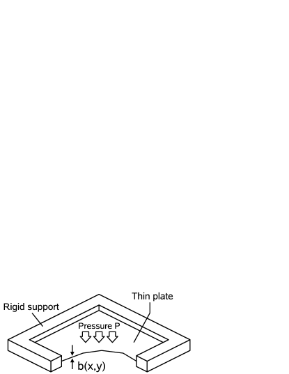
Figure 1: Cutaway view of a thin pressure-supporting plate which spans a square aperture, and is clamped at the edges of this to a rigid support.

II Precise statement of the problem

Consider a thin plate of elastic material with Young modulus $Y$ and Poisson ratio $\nu$. We assume that when the plate is not subject to a pressure load, it has no quenched-in stresses, it lies in the $x-y$ plane, and has a possibly non-uniform thickness $b(x,y)$.

The plate is attached to the boundary of a rigid aperture, so that even under load, the out-of-plane deflection and its gradient are zero at the boundary. We refer to these constraints as “cantilever boundary conditions”.

Let $L_{0}$ be a typical unit of length (for example of the same order of magnitude as the size of the aperture), then we assume that the plate is thin, in the sense that $b/L_{0}\ll 1$. Let us suppose that the plate is now subject to a small pressure difference $P$ between its two sides, and we define a non-dimensional pressure loading parameter $p=P/Y$.

In order to state the problem, we first need an expression for the elastic energy of the plate under such pressure loading. We are furthermore interested in the case where the deflection of the plate may not be small compared to its thickness, and we will therefore have to consider stretching or shearing of the middle plane of the plate Timoshenko .

Under these circumstances, a useful approximation is that of von Karman vonKarman ; Timoshenko . A simple exposition may also be found in Ref. Lobkovsky , from which we take (with a change of notation) the results we need below.

Consider a region of the middle plane of the plate near a point which has co-ordinates before loading given by $(x_{0},y_{0},0)$. Under a load $p$, the plate will deform, after which we define the new co-ordinates of the point under consideration to be

$$\left(x_{0}+u(x_{0},y_{0}),y_{0}+v(x_{0},y_{0}),w(x_{0},y_{0})\right),$$

where $u$, $v$ and $w$ are assumed to be small and we have allowed the possibility of out-of-plane deformations $w$.

The two-dimensional strain tensor of the middle layer after deformation is given by ${\rm\bf e}$ with components

$$e_{xx}=\frac{\partial u}{\partial x_{0}}+\frac{1}{2}\left(\frac{\partial w}{\partial x_{0}}\right)^{2}$$

$$e_{xy}=\frac{1}{2}\frac{\partial u}{\partial y_{0}}+\frac{1}{2}\frac{\partial v}{\partial x_{0}}+\frac{1}{2}\left(\frac{\partial w}{\partial x_{0}}\right)\left(\frac{\partial w}{\partial y_{0}}\right)$$

$$e_{yy}=\frac{\partial v}{\partial y_{0}}+\frac{1}{2}\left(\frac{\partial w}{\partial y_{0}}\right)^{2}.$$

For a uniformly thick plate (or a plate with sufficiently slowly varying thickness Timoshenko2 ) the equilibrium deformation of the middle plane can be obtained by minimising the energy $U$ of Eq. (1) with suitable boundary conditions Lobkovsky , where

$$U=U_{S}+U_{B}-Y\int{dxdy(pw)}.$$ (1)

and the stretching and bending energies of the plate can be simply derived from the corresponding expressions in Ref. Lobkovsky as:

$$U_{S}=\int dxdy\frac{Yb}{2(1-\nu^{2})}\left\{\nu\left[{\rm Tr}({\rm\bf e})\right]^{2}+(1-\nu){\rm Tr}({\rm\bf e}^{2})\right\}$$ (2)

$$U_{B}=\int dxdy\frac{Yb^{3}}{24(1-\nu^{2})}\left\{\left[{\rm Tr}(H)\right]^{2}-2(1-\nu){\rm det}(H)\right\}$$ (3)

where $H$ is the Hessian matrix

$$H(x,y)=\left(\begin{array}[]{cc}\frac{\partial^{2}w}{\partial x^{2}}&\frac{\partial^{2}w}{\partial x\partial y}\\ \frac{\partial^{2}w}{\partial x\partial y}&\frac{\partial^{2}w}{\partial y^{2}}\end{array}\right).$$ (4)

In addition to this, we note that the maximum tensile strain experienced by the material is given by

$$e_{\max}=\max_{\theta}\left[\hat{\bf q}^{T}{\bf e}\hat{\bf q}+\frac{b}{2}\left|\hat{\bf q}^{T}\left(\begin{array}[]{cc}\partial_{x}^{2}w&\partial_{xy}^{2}w\\ \partial_{xy}^{2}w&\partial_{y}^{2}w\end{array}\right)\hat{\bf q}\right|\right],$$ (5)

where $\hat{\bf q}^{T}=(\cos\theta,\sin\theta)$. In this expression, the first term comes from stretching from in- and out-of-plane deformation of the middle plane and the second from stretching produced by bending of the plate (which is maximal at a distance $\pm b/2$ from the middle plane).

In what follows, we assume that the material is brittle, in that it will fail if it experiences a tensile strain that exceeds a small number $\epsilon\ll 1$. We therefore have the no-breaking condition:

$$e_{\max}\leq\epsilon$$ (6)

We can now state precisely the problem of finding a mechanically efficient plate: for a fixed aperture geometry, and for each pair of values $(\epsilon,p)$, we wish to find that function $b(x,y)$ which minimises the integral $\int{b(x,y)}dxdy$, while at the same time achieving mechanical equilibrium (minimising the energy of Eq. (1)) and subject to the condition of no breakage in Eq. (6). In fact, this problem as stated is not well-posed; we therefore choose the extra restriction (discussed in section IV.1) that $|\nabla b|\leq G$ everywhere, for some fixed number $G$.

It is tempting to approach this problem by choosing an arbitrary function $b(x,y)$, minimising the energy, and then locally removing or adding material according as whether $e_{\max}$ is greater than or less than $\epsilon$. This is a possible strategy, but based on the calculations to follow we suspect that starting from a uniform $b$, this strategy will only produce a local minimum in the amount of material used.

III One dimensional case

III.1 Solution for cantilever boundary conditions

Let us consider the case where we have a plate which is infinitely long in the $y$-direction. Furthermore, we impose the strong restriction that $b$ is a function only of $x$, the direction across the plate. This will turn out to be very sub-optimal, but it is an instructive case for developing the argument. Under these conditions, $v=0$, while $u$, $w$ and $b$ are functions only of $x$. The energy per unit length in the $y$-direction of the plate under pressure becomes

$$U=\frac{Y}{1-\nu^{2}}\int{dx}\left[\frac{b}{2}(\partial_{x}u)^{2}+\frac{b}{2}(\partial_{x}u)(\partial_{x}w)^{2}\right.$$

$$\left.\frac{b}{8}(\partial_{x}w)^{4}+\frac{b^{3}}{24}(\partial_{x}^{2}w)^{2}-(1-\nu^{2})pw\right],$$ (7)

which must be minimised subject to the no-breakage condition

$$\frac{\partial u}{\partial x}+\frac{1}{2}\left(\frac{\partial w}{\partial x}\right)^{2}+\frac{b}{2}\left|\frac{\partial^{2}w}{\partial x^{2}}\right|\leq\epsilon.$$ (8)

As stated above, the material is brittle in the sense $\epsilon\ll 1$, and we want the plate to be thin ($b/L_{0}\ll 1$). We also expect $u/L_{0}\ll 1$, $w/L_{0}\ll 1$, and from the geometry, $O(u)=O(w^{2})$, which we write for brevity as $u\sim w^{2}$.

Now, consider first the case where $b$ is a constant and the plate is a strip given by $x\in(-a,a)$. Let $\xi\equiv x/a$ then the Euler-Lagrange equations obtained by minimising the energy of Eq. (III.1) are

$$\frac{\partial u}{\partial\xi}=a\frac{b^{2}}{a^{2}}\frac{\zeta^{2}}{12}-\frac{1}{2a}\left(\frac{\partial w}{\partial\xi}\right)^{2},$$ (9)

$$\frac{\partial^{4}w}{\partial\xi^{4}}=\zeta^{2}\frac{\partial^{2}w}{\partial\xi^{2}}+12a\left(\frac{a}{b}\right)^{3}\tilde{p},$$ (10)

where $\tilde{p}\equiv(1-\nu^{2})p$ and $\zeta$ is the constant of integration of the Euler-Lagrange equations which is still to be determined (physically, $\zeta$ has the interpretation that $\zeta^{2}b^{2}/(12a^{2})$ is the strain experienced by the mid-plane of the plate).

Noting that $w=\partial_{x}w=0$ at $x=\pm a$, and that $w$ is symmetric about $x=0$, we find

$$w=\frac{6a\tilde{p}}{\zeta^{2}}\left(\frac{a}{b}\right)^{3}\left[(1-\xi^{2})+\frac{2\left[\cosh(\zeta\xi)-\cosh\zeta\right]}{\zeta\sinh\zeta}\right]$$ (11)

$$u=a\frac{b^{2}\zeta^{2}}{12a^{2}}\xi-\frac{72a\tilde{p}^{2}}{\zeta^{4}}\left(\frac{a}{b}\right)^{6}\left[\frac{\xi^{3}}{3}-\frac{2\xi\cosh(\zeta\xi)}{\zeta\sinh\zeta}\right.$$

$$\left.+\frac{2\sinh(\zeta\xi)}{\zeta^{2}\sinh\zeta}+\frac{\sinh(2\zeta\xi)-2\zeta\xi}{4\zeta\sinh^{2}\zeta}\right].$$ (12)

The condition which determines $\zeta$ is that $u=0$ at $x=\pm a$, which gives

$$1=\frac{864\tilde{p}^{2}}{\zeta^{6}}\left(\frac{a}{b}\right)^{8}\left[\frac{1}{3}-\frac{2\cosh\zeta}{\zeta\sinh\zeta}+\frac{2}{\zeta^{2}}+\frac{\sinh(2\zeta)-2\zeta}{4\zeta\sinh^{2}\zeta}\right].$$ (13)

The Euler-Lagrange equation, Eq. (9) for $u$ shows that the strain produced by stretching at the middle plane is uniform over the plate, and therefore the no-breakage condition is

$$\frac{\zeta^{2}b^{2}}{12a^{2}}+\frac{b}{2a^{2}}\left|\frac{\partial^{2}w}{\partial\xi^{2}}\right|\leq\epsilon.$$ (14)

III.1.1 Breakage dominated by stretching: $\zeta$ large

Consider first the case $\zeta$ large, which corresponds to $\tilde{p}a^{4}/b^{4}\gg 1$, then bending occurs mainly in thin “boundary layers” near the edges of the plate (i.e. close to $\xi=1$ and $\xi=-1$) which have a width $\Delta\xi\sim 1/\zeta$. In this limit, we find

$$\zeta\approx(288)^{1/6}\tilde{p}^{1/3}\left(\frac{a}{b}\right)^{4/3}.$$ (15)

From the no-breakage condition of Eq. (14), we can calculate the required thickness of the plate. We find that bending and stretching both contribute significantly in the boundary layer (but bending is unimportant elsewhere), and the necessary minimum thickness $b_{\min}$ is

$$\left(\frac{b_{\min}}{a}\right)\approx 2.885\tilde{p}\epsilon^{-3/2}.$$ (16)

It is also interesting to know $\zeta$ in terms of $\tilde{p}$ and $\epsilon$ for the case when $b=b_{\min}$, in order to estimate the thickness of the boundary layers. The result is

$$\zeta\approx 0.626\epsilon^{2}\tilde{p}^{-1}.$$

Lastly, consistency with the fact that $\tilde{p}a^{4}/b^{4}\gg 1$ implies that $\tilde{p}\ll\epsilon^{2}$.

III.1.2 Breakage dominated by bending: $\zeta$ small

Next, let us consider the opposite extreme, where breakage is dominated by bending everywhere; i.e. $\zeta$ is very small, equivalent to $\tilde{p}a^{4}/b^{4}\ll 1$. This leads to

$$\zeta\approx\frac{8}{\sqrt{35}}\tilde{p}\left(\frac{a}{b}\right)^{4}.$$

There are no boundary layers, and the expression for $w$ becomes

$$w\approx\frac{a\tilde{p}}{2}\left(\frac{a}{b}\right)^{3}\left(1-\xi^{2}\right)^{2}.$$

The no-breakage condition is therefore:

$$\frac{\zeta^{2}b^{2}}{12a^{2}}+\frac{2\tilde{p}a^{2}}{b^{2}}\leq\epsilon,$$

where the first term corresponds to strain from stretching of the middle layer (both in-plane and out-of-plane), and the second term is strain from bending. We find that breakage is governed only by the bending term in this limit, and

$$\left(\frac{b_{\min}}{a}\right)\approx 2^{1/2}\tilde{p}^{1/2}\epsilon^{-1/2}.$$

Consistency with $\tilde{p}a^{4}/b^{4}\ll 1$ leads to $\tilde{p}\gg\epsilon^{2}$, and thinness of the plate $(b/a)\ll 1$ also imposes the condition $\tilde{p}\ll\epsilon$.

III.2 Freely hinged boundary conditions

In the case of $\zeta$ large, the required minimum thickness of a uniform plate is determined by the thickness needed to sustain the bending and stretching forces in the thin boundary layers at the edges of the plate. Given more freedom to design a plate with non-uniform thickness, one might imagine that the most efficient design would have a larger value for $b$ in the two boundary layers near the edges, and be thinner everywhere else. The required thickness of this middle region could be estimated conservatively from the minimum thickness required for a plate with freely hinged boundary conditions. This case is also immediately solvable: we require that $w$ be symmetrical while $u=0$, $w=0$ and $\partial_{x}^{2}w=0$ at $x=\pm a$. The Euler-Lagrange equations Eq. (9) and (10) then give in the limit of large $\zeta$

$$\left(\frac{b_{\min}}{a}\right)\approx 0.408\tilde{p}\epsilon^{-3/2}.$$ (17)

The important thing to note is that although the pre-factor is smaller in Eq. (17), the order of magnitude of all quantities is the same as for the cantilevered boundary condition case (Eq. (16)). Even if we were to optimise the mechanical efficiency of the plate by choosing $b$ to be thicker in the boundary layer and thinner in the centre of the plate, we would only achieve a gain in efficiency by a numerical factor of order unity. We also conjecture that an optimisation strategy comprising removing material where the breakage condition is not satisfied will converge on a solution of this kind.

The boundary layers we encounter in this case are therefore in some sense unimportant; having only a quantitative and not a qualitative effect on the amount of material needed to make our pressure-bearing plate. Shortly however, we shall encounter cases where the presence of boundary layers (regions where quantities vary rapidly in space) alters even the scaling of mechanical efficiency with $p$ and $\epsilon$.

III.3 Order of magnitude behaviour for a uniform plate

We can now state the order-of-magnitude behaviour of various quantities (assuming $\nu\neq-1$) for our optimum thin plate which has either uniform thickness, or boundary layers at the edges. In what follows, we shall use “$\sim$” to denote that two quantities are the same order of magnitude. We have:

$$\left(\frac{b_{\min}}{a}\right)\sim\left\{\begin{array}[]{cc}p\epsilon^{-3/2}&p\ll\epsilon^{2}\\ p^{1/2}\epsilon^{-1/2}&\epsilon^{2}\ll p\ll\epsilon\end{array}\right.,$$ (18)

where the first case corresponds to a stretching-dominated and the second to a bending-dominated regime.

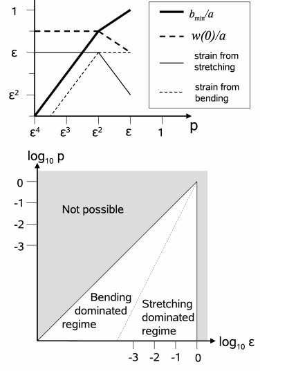
Figure 2: Top figure: order of magnitude behaviour for quantities as a function of pressure, for an aperture spanned by a plate of uniform thickness. Plotted on this scale, all crossovers are sharp and all order 1 prefactors are invisible. Bottom figure: schematic picture of the $p-\epsilon$ plane, showing the approximate positions of crossovers in behaviour for this case. The dashed line showing the crossover of regimes is $p\sim\epsilon^{2}$

The maximum deflection, maximum curvature from bending and maximum strain from stretching (both in-plane and out of plane) are given by

$$\left(\frac{w(0)}{a}\right)\sim\left\{\begin{array}[]{cc}\epsilon^{1/2}&p\ll\epsilon^{2}\\ p^{-1/2}\epsilon^{3/2}&\epsilon^{2}\ll p\ll\epsilon\end{array}\right.,$$ (19)

$$b\left.\frac{\partial^{2}w}{\partial x^{2}}\right|_{\max}\sim\left\{\begin{array}[]{ccc}\epsilon&p\ll\epsilon^{2}&{\rm in\ b.\ layer}\\ p\epsilon^{-1}&p\ll\epsilon^{2}&{\rm out\ b.\ layer}\\ \epsilon&\epsilon^{2}\ll p\ll\epsilon&\end{array}\right.,$$ (20)

$$\frac{\zeta^{2}b^{2}}{a^{2}}\sim\left\{\begin{array}[]{cc}\epsilon&p\ll\epsilon^{2}\\ p^{-1}\epsilon^{3}&\epsilon^{2}\ll p\ll\epsilon\end{array}\right..$$ (21)

These relations are shown in the top panel of Fig. 2 as an “order of magnitude” (“o.o.m.”) plot. The advantage of the compressed scale used in this plot is that all crossover behaviour is sharp, and prefactors are irrelevant (indeed even a factor as large as $\log(\epsilon^{-1})$ would be invisible on this scale). The bottom panel of Fig. 2 shows the different regimes in the $p-\epsilon$ plane. Because of the different scale, pre-factors are now important, and so the picture must be regarded as schematic (except very far from the origin at $(\log\epsilon,\log p)=(0,0)$ ).

IV Plate with parallel spars

IV.1 Behaviour of a single spar

So far we have analysed the case where the thickness $b$ is constant, or (by arguing from these solutions), the case where there are narrow boundary layers at the edges of the plate accommodating the local bending forces. However, because the bending term (Eq. (3)) in the energy (Eq. (1)) has a pre-factor cubic in the plate thickness, we expect intuitively that it would be more efficient still to design a plate with narrow, thick (large $b$) beams or “spars”, which support thinner “panels” between. A simple example of such a design would be as shown in Fig. 3.

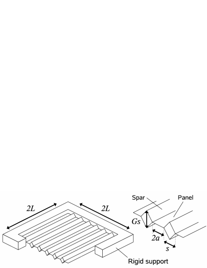
Figure 3: Schematic for the design of a plate consisting of parallel spars separated by long narrow panels, and spanning a square aperture of side $2L$.

Again, from the form of the energy expression, we would expect that the design would get more efficient the narrower (smaller $s$ in Fig. 3) and the taller (larger $Gs$ in Fig. 3) the supporting spars are designed to be. However, at some point, very narrow and tall spars are likely to buckle under loading. In the analysis that follows, we have therefore placed a simple restriction on the design of the plate, which is both interesting in its own right, but can also be seen as an attempt to capture this buckling limitation. The design restriction we place is that the maximum gradient of the thickness cannot exceed some set value $G$, which is of order unity. There is also a third reason for choosing such a $G$, which represents a limitation of the current analysis, rather than a change in the qualitative beahviour of the system. This limitation is that if the thickness $b$ varies too quickly in space, then Eqs. (2) and (3) will no longer be valid.

Stated formally the new restriction is that

$$\forall(x,y):\left|\nabla b(x,y)\right|\leq G.$$ (22)

Let us therefore consider a spar which has a diamond-shaped cross section satisfying this constraint, with width $s$, length $2L$ and loaded under a force $\tilde{f}$ per unit length. We define a re-scaled parameter with dimensions of length to describe this loading, namely $f=\tilde{f}/Y$.

In order to write down the energy of this system from Eq. (1), we need a further condition on the deformation of the middle plane. Because we are envisaging a narrow spar, we take this condition to be that the component of the stress in the $x$-direction (across the spar) at the middle plane is zero. Because the $x$ and $y$ directions are still the principal directions for both the strain and stress tensor, then this leads to $e_{xx}=-\nu e_{yy}$ and so the energy of the spar is given by

$$U=Y\int{dy}\left\{\frac{Gs^{2}}{4}\left[\partial_{y}v+\frac{1}{2}(\partial_{y}w)^{2}\right]^{2}\right.$$

$$\left.+\frac{G^{3}s^{4}}{192}\frac{(\partial_{y}^{2}w)^{2}}{(1-\nu^{2})}-fw\right\}.$$ (23)

Defining $\eta\equiv y/L$, the Euler-Lagrange equations for Eq. (IV.1) are

$$\frac{\partial v}{\partial\eta}=L\frac{\zeta^{2}G^{2}s^{2}}{48L^{2}(1-\nu^{2})}-\frac{1}{2L}\left(\frac{\partial w}{\partial\eta}\right)^{2},$$

$$\frac{G^{2}s^{2}}{48L^{2}}\frac{\partial^{4}w}{\partial\eta^{4}}=\frac{\zeta^{2}G^{2}s^{2}}{48L^{2}}\frac{\partial^{2}w}{\partial\eta^{2}}+\frac{2f(1-\nu^{2})L^{2}}{Gs^{2}},$$

where $\zeta$ is a constant of integration in the Euler-Lagrange equations for Eq. (IV.1) and needs to be determined. Solving these with cantilever boundary conditions gives

$$w=\frac{48L^{4}(1-\nu^{2})f}{G^{3}s^{4}\zeta^{2}}\left[(1-\eta^{2})+\frac{2\left[\cosh(\zeta\eta)-\cosh\zeta\right]}{\zeta\sinh\zeta}\right],$$

$$v=\frac{\zeta^{2}G^{2}s^{2}}{48L(1-\nu^{2})}\eta$$

$$-\frac{4608L^{7}(1-\nu^{2})^{2}f^{2}}{G^{6}s^{8}\zeta^{4}}\left[\frac{\eta^{3}}{3}-\frac{2\eta\cosh(\zeta\eta)}{\zeta\sinh\zeta}\right.$$

$$\left.+\frac{2\sinh(\zeta\eta)}{\zeta^{2}\sinh\zeta}+\frac{\sinh(2\zeta\eta)-2\zeta\eta}{4\zeta\sinh^{2}\zeta}\right],$$

where the constant of integration $\zeta$ can be determined from

$$\frac{G^{8}s^{10}}{L^{8}f^{2}}=\frac{221184(1-\nu^{2})^{3}}{\zeta^{6}}$$

$$\times\left[\frac{1}{3}-\frac{2\cosh\zeta}{\zeta\sinh\zeta}+\frac{2}{\zeta^{2}}+\frac{\sinh(2\zeta)-2\zeta}{4\zeta\sinh^{2}\zeta}\right].$$

From now on, we consider only the orders of magnitudes of different quantities, and again there will be two cases:

IV.1.1 Stretching dominated regime

In the stretching dominated regime, we have $\zeta\gg 1$, and

$$\zeta\sim\frac{L^{4/3}f^{1/3}}{G^{4/3}s^{5/3}},$$

so $f\gg G^{4}s^{5}/L^{4}$ and the no-breaking condition (which is dominated by stre tching everywhere except at the ends of the spar, where bending is also significant) gi ves

$$f\leq\epsilon^{3/2}s^{2}L^{-1}G.$$

Because of the no-breakage condition, the strain from in-plane and out-of-plane stretching is always less than $\epsilon$. The maximum amount of bending is

$$\left.\frac{\partial^{2}w}{\partial y^{2}}\right|_{\max}\sim\frac{L^{2}f}{G^{3}s^{4}\zeta}\sim\frac{L^{2/3}f^{2/3}}{G^{5/3}s^{7/3}},$$

which occurs in the “boundary layers” near the two ends of the spar. The maximum out-of-plane deflection is

$$w(0)\sim\frac{L^{4/3}f^{1/3}}{G^{1/3}s^{2/3}}.$$

IV.1.2 Bending dominated regime

In the case that $\zeta$ is small, we are in the bending dominated regime and we find that

$$\zeta\sim\frac{L^{4}f}{G^{4}s^{5}}$$

Therefore consistency requires that $f\ll G^{4}s^{5}/L^{4}$ and the no-breaking condition (which is dominated by bending) is

$$f\leq\epsilon s^{3}L^{-2}G^{2}.$$

The maximum amount of bending is given by

$$\left.\frac{\partial^{2}w}{\partial y^{2}}\right|_{\max}\sim\frac{L^{2}f}{G^{3}s^{4}}$$

and the amount of in-plane and out-of-plane stretching is of order

$$\frac{\zeta^{2}G^{2}s^{2}}{L^{2}}\sim\frac{L^{6}f^{2}}{G^{6}s^{8}}.$$

The maximum out-of plane deflection is

$$w(0)\sim\frac{L^{4}f}{G^{3}s^{4}}.$$

IV.2 Parallel spars supporting panels

Let us suppose we have a plate consisting, as in Fig. 3, of parallel “spars” separated by thinner “panels”. The parallel spars also represent a collection of boundary layers for the function $b(x,y)$, in the sense that quantities have a fast variation as a function of $x$ or $y$. In contrast to the case discussed above, these boundary layers produce a qualitative change in the system’s behaviour.

We assume that the entire aperture is a square of side $2L$, and that the spars are of width $s$, and separated by a distance $2a$ from neighbouring spars. Because the analysis from now on will focus on orders of magnitude, we shall assume that $G$ is of order unity, and omit it from the expressions. We will assume (and later check) that $s\ll a$ and $a\ll L$ (the latter, together with the relative rigidity of the spars, ensuring that we can treat the panels as infinitely long strips). The panels have a thickness $b_{0}$.

We now calculate the average thickness $\langle b\rangle$ of the plate that is required to support a pressure load, where (again in order-of-magnitude terms)

$$\langle b\rangle\sim\frac{ab_{0}+s^{2}}{a+s}\sim\frac{\max(ab_{0},s^{2})}{\max(a,s)},$$ (24)

and the second equivalence follows from the fact that the terms being added (in each of the numerator and denominator) will in general be of different magnitude.

Because $s\ll a$, then over almost all their length, the spars must support a force per unit length given by $f=2ap$.

We consider the four cases where the spars and panels are in the stretching and bending dominated regimes. There are six conditions which have to be applied in each case:

(i) The panels are assumed to be at their most mechanically efficient, which sets $b_{0}$ as a function of $p$ and $a$.

(ii) Whether the panels are in the bending or stretching dominated regime sets a constraint on the pressure.

(iii) The spars are in the stretching dominated regime if $ap\gg s^{5}/L^{4}$ and the bending dominated regime if $ap\ll s^{5}/L^{4}$.

(iv) The spars must not break (although we do not insist that they should be at this limit; they may be somewhat over-engineered in this sense).

(v) The spars must provide significant support, in the sense that the maximum out-of-plane displacement at the centre of each spar must be much less than the maximum out-of-plane displacement at the centre of each panel.

(vi) There must be at least one spar in the system; in other words $(a/L)\leq 1$.

These conditions are listed in Table 1.

Table 1: The six conditions which must be satisfied by spars and panels for a plate consisting of parallel spars supporting intervening panels. Spars and panels may be either in the bending or stretching dominated regimes.

	Spars in stretching	Spars in bending
	dominated regime	dominated regime
	$b_{0}\sim ap\epsilon^{-3/2}$	$b_{0}\sim ap\epsilon^{-3/2}$
Panels in	$p\ll\epsilon^{2}$	$p\ll\epsilon^{2}$
stretching	$\left(\frac{s}{L}\right)\ll\left(\frac{a}{L}\right)^{1/5}p^{1/5}$	$\left(\frac{s}{L}\right)\gg\left(\frac{a}{L}\right)^{1/5}p^{1/5}$
dominated	$\left(\frac{s}{L}\right)\geq\left(\frac{a}{L}\right)^{1/2}p^{1/2}\epsilon^{-3/4}$	$\left(\frac{s}{L}\right)\geq\left(\frac{a}{L}\right)^{1/3}p^{1/3}\epsilon^{-1/3}$
regime	$\left(\frac{s}{L}\right)\gg\left(\frac{a}{L}\right)^{-1}p^{1/2}\epsilon^{-3/4}$	$\left(\frac{s}{L}\right)\gg p^{1/4}\epsilon^{-1/8}$
	$(a/L)\leq 1$	$(a/L)\leq 1$
	$b_{0}\sim ap^{1/2}\epsilon^{-1/2}$	$b_{0}\sim ap^{1/2}\epsilon^{-1/2}$
Panels in	$\epsilon^{2}\ll p\ll\epsilon$	$\epsilon^{2}\ll p\ll\epsilon$
bending	$\left(\frac{s}{L}\right)\ll\left(\frac{a}{L}\right)^{1/5}p^{1/5}$	$\left(\frac{s}{L}\right)\gg\left(\frac{a}{L}\right)^{1/5}p^{1/5}$
dominated	$\left(\frac{s}{L}\right)\geq\left(\frac{a}{L}\right)^{1/2}p^{1/2}\epsilon^{-3/4}$	$\left(\frac{s}{L}\right)\geq\left(\frac{a}{L}\right)^{1/3}p^{1/3}\epsilon^{-1/3}$
regime	$\left(\frac{s}{L}\right)\gg\left(\frac{a}{L}\right)^{-1}p^{5/4}\epsilon^{-9/4}$	$\left(\frac{s}{L}\right)\gg p^{3/8}\epsilon^{-3/8}$
	$(a/L)\leq 1$	$(a/L)\leq 1$

Table 2: The scaling properties of optimally efficient plates consisting of parallel spars supporting intervening panels. Spars and panels may be either in the bending or stretching dominated regimes.

	Spars in stretching	Spars in bending
	dominated regime	dominated regime
Panels in	$p\ll\epsilon^{5/2}$	$\epsilon^{5/2}\ll p\ll\epsilon^{2}$
stretching	Spars give	$\langle b\rangle\sim Lp^{3/4}\epsilon^{-7/8}$
dominated	no gain	$\left(\frac{s}{L}\right)\sim p^{1/4}\epsilon^{-1/8}$
regime	in efficiency	$\left(\frac{a}{L}\right)\sim p^{-1/4}\epsilon^{5/8}$
Panels in	Not	$\epsilon^{2}\ll p\ll\epsilon$
bending	consistent	$\langle b\rangle\sim Lp^{5/8}\epsilon^{-5/8}$
dominated	with	$\left(\frac{s}{L}\right)\sim p^{3/8}\epsilon^{-3/8}$
regime	conditions	$\left(\frac{a}{L}\right)\sim p^{1/8}\epsilon^{-1/8}$

It is a simple, but tedious matter to combine the conditions of Table 1 with Eq. (24) to obtain the scaling properties of the optimally efficient solution in each case. The results are shown in Table 2.

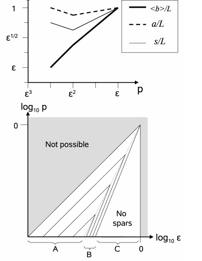
Figure 4: Top figure: order of magnitude behaviour for quantities as a function of pressure for an aperture spanned by a plate consisting of parallel spars supporting long panels. Bottom figure: schematic picture of the $p-\epsilon$ plane, showing contours (solid lines) of constant number of spars in the structure. This number increases towards the bottom left of the figure. Region ‘A’ is where spars and panels are bending dominated ($\epsilon^{2}\ll p\ll\epsilon$). Region ‘B’ is where spars are bending dominated and panels are stretching dominated ($\epsilon^{5/2}\ll p\ll\epsilon^{2}$), and region ‘C’ is where there are no spars, and the now uniformly thick plate is stretching dominated ($p\ll\epsilon^{5/2}$).

Fig. 4 shows these behaviours on an o.o.m. plot, and (schematically) on the $p-\epsilon$ plane.

V Fractal design

V.1 Two beams at right angles

The parallel spars analysed above have provided considerable gains in efficiency over a uniform plate, but it is possible that we have not achieved the global optimal scaling. One possibility which remains is that we could allow spars to intersect. In this way, thicker spars may be used to partially support thinner spars, which together support panels. We can envisage ultimately a hierarchical arrangement with spars of progressively thinner aspect forming a fractal design, and supporting panels only at the smallest length scales.

To proceed, we first investigate whether the principle of a thicker spar supporting a thinner spar can indeed lead to a gain in efficiency for a structure. Consider therefore a single spar which is in the bending dominated regime, carrying a (scaled) force $f$ per unit length, and a point load $\tilde{F}$ at the centre, which we represent by a scaled point force $F=\tilde{F}/Y$. The spar or beam must be considered in two sections, joined at the middle ($x=0$), at which point the displacement $w$ and the first two derivatives of $w$ are continuous

$$w(x)=\left\{\begin{array}[]{cc}w^{+}(x)&x\in(0,L)\\ w^{-}(x)&x\in(-L,0)\end{array}\right.$$ (25)

Hence, if we have two beams at right angles with widths $s_{1}$ and $s_{2}$, joined at the centre, and each carrying a force $f$ per unit length, they will (in the absence of external point forces) apply equal and opposite forces $F$ on each other, and their displacements will be given by the following expressions:

$$w_{1}^{\pm}(x)=\frac{4f}{G^{3}s_{1}^{4}}\left(x^{2}-L^{2}\right)^{2}\pm\frac{8F}{G^{3}s_{1}^{4}}\left(x\mp L\right)^{2}\left(x\pm\frac{L}{2}\right)$$

$$w_{2}^{\pm}(y)=\frac{4f}{G^{3}s_{2}^{4}}\left(y^{2}-L^{2}\right)^{2}\mp\frac{8F}{G^{3}s_{2}^{4}}\left(y\mp L\right)^{2}\left(y\pm\frac{L}{2}\right)$$

$$F=fL\left(\frac{s_{1}^{4}-s_{2}^{4}}{s_{1}^{4}+s_{2}^{4}}\right),$$ (26)

where the point force $F$ in Eq. (26) imposes the constraint that the beams must have the same displacement $w(0)$ at their centre points.

For this highly symmetrical case, the maxima in curvature occur either at the ends or the centres of the beams (for more general cases, there may be maxima between the positions of application of point loads). We can therefore write the no-breakage condition on the first beam as

$$\frac{Gs_{1}}{2}\left|\partial_{x}^{2}w_{1}^{\pm}(x)\right|_{\max}=$$

$$\frac{4fL^{2}}{G^{2}s_{1}^{3}(r^{4}+1)}\max\left[\left|5r^{4}-1\right|,(7r^{4}+1)\right]\leq\epsilon$$

or

$$\frac{s_{1}^{3}}{L^{3}}\geq\frac{4f}{(r^{4}+1)LG^{2}\epsilon}\max\left[\left|5r^{4}-1\right|,(7r^{4}+1)\right],$$ (27)

where $r\equiv s_{1}/s_{2}$. The result must be symmetric on swapping the two spars, so

$$\frac{s_{2}^{3}}{L^{3}}\geq\frac{4f}{(r^{-4}+1)LG^{2}\epsilon}\max\left[\left|5r^{-4}-1\right|,(7r^{-4}+1)\right].$$ (28)

The total volume of material used to make these beams is therefore

$$V=GL\left(s_{1}^{2}+s_{2}^{2}\right),$$ (29)

which we seek to minimise.

Eqs. (27) and (28) have a trivial solution in which $s_{1}=s_{2}$ and $F=0$. The most efficient solution of this kind has both beams at the breaking limit, so

$$s_{1}=s_{2}=2^{4/3}L(f/L)^{1/3}\epsilon^{-1/3}G^{-2/3},$$ (30)

and uses a volume of material given by

$$V\approx 12.699L^{3}(f/L)^{2/3}\epsilon^{-2/3}G^{-1/3}.$$ (31)

However, this is not the global optimum, which in fact occurs when $r\approx 1.22$ and

$$V\approx 12.652L^{3}(f/L)^{2/3}\epsilon^{-2/3}G^{-1/3},$$ (32)

and only the thinner of the two beams is at its breaking limit.

We therefore see that although the gains are very modest, it is nevertheless possible to achieve greater efficiency through having a thicker beam or spar support a thinner. The next question to address is whether this principle can be extended to a hierarchical arrangement with thin spars supporting still thinner spars, until the very thinnest help to support panels to form a continuous plate with no holes.

V.2 Hierarchical arrangement of spars

Consider the arrangement of spars as shown in Fig. 5. Fig. 5(a) shows two spars at right angles, and we refer to this structure as “generation 1”. We choose the spars to have the same width $s_{1,1}$ (the first index referring to the “generation number”, and the second to the type of spar present in this generation). Each spar carries a force per unit length $f_{1}=f_{0}/2$. In light of the previous calculation, we know that it is not optimal to have both spars of the same width; but we ignore this fact in favour of simplicity of analysis.

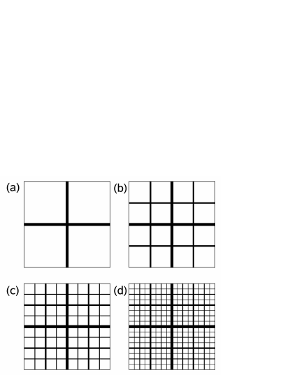
Figure 5: Schematic of a fractal design for a plate spanning a square aperture. (a) is a “generation 1” structure, with two crossed spars supporting four panels. In (b), four thinner spars are added, which subdivides the remainder of the plate into sixteen panels. In (c) and (d) we show generations 3 and 4.

Fig 5(b) shows a “generation 2” structure, where we have two thick spars, just as for generation 1, but their widths are now $s_{2,1}$ which may be different from $s_{1,1}$. In addition, there are four thinner spars, each with width $s_{2,2}$. All the spars now carry a force per unit length of $f_{2}=f_{0}/4$ – chosen to approximate the loading produced by the smaller panels between the spars which will eventually be present in the structure. Fig. 5(c) and (d) show generations 3 and 4 respectively, and we envisage going to large generation numbers $n$ for certain regions of the $p-\epsilon$ plane.

For generation $n$, we will have two spars of width $s_{n,1}$, four thinner spars of width $s_{n,2}$ and so on, culminating with $2^{n}$ of the thinnest spars, which each have a width $s_{n,n}$. The total number of spars in the generation $n$ structure is therefore $2(2^{n}-1)$, and each carries a force per unit length (in addition to the point forces) of $f_{n}=2^{-n}f_{0}$. Again, this is chosen to mimic the loading on the spars produced by supported panels, so that $f_{0}\approx pL/4$ (although the loading in this final structure will not be exactly uniform).

We now analyse the first few generations numerically, ignoring the possible torsional loadings that spars can exert upon one another in asymmetrical configurations. We expect this complication to have minimal effects when $G\lesssim 1$, and so we now specialise to the case $G=1$.

For generation $n$, we choose a structure described by the two parameters $\beta(n)$ and $\gamma(n)$ defined by

$$s_{n,q}=L\left(\frac{f_{0}}{L}\right)^{1/3}\epsilon^{-1/3}\beta(n)\left[\gamma(n)\right]^{q-1}.$$ (33)

We choose $\beta(n)$ and $\gamma(n)$ so that all the spars satisfy the no-breaking condition, and the amount of material V that is used, is minimised. Adding up the total volume of material in the spars gives

$$V(n)=2L^{3}\left(\frac{f_{0}}{L}\right)^{2/3}\epsilon^{-2/3}\beta^{2}(n)\left\{\frac{\left[2\gamma^{2}(n)\right]^{n}-1}{2\gamma^{2}(n)-1}\right\}.$$ (34)

Based on experience from the previous section, we expect that the most efficient structure of this kind will satisfy the breakage condition as an equality only for the thinnest spars. We also expect $\gamma(n)>0.5$ (the thicker spars will not act as completely rigid supports for the thinner spars), but we hope that a hierarchical structure is still achieved, which corresponds to $\gamma(n)<1$.

Table 3 shows the first few values for $\beta(n)$ and $\gamma(n)$ which are found from numerical simulations to minimise $V(n)$. The tentative conclusion is that both quantities tend to fixed, order 1 values as $n$ increases.

Table 3: Values for $\beta(n)$ and $\gamma(n)$ (in Eq. (33)) which are found numerically to minimise $V(n)$ (Eq. (34) from the text).

$n$	$\beta(n)$	$\gamma(n)$
1	1.260	$-$
2	1.126	0.609
3	1.009	0.644
4	1.078	0.650

If now we assume that $\beta(n)$ and $\gamma(n)$ do indeed tend to fixed limits $\beta$ and $\gamma$ as $n\rightarrow\infty$, then provided the spars remain much narrower than the panels, and the spars remain in the bending dominated regime, we can calculate the average thickness of the plate. It will be a sum of two terms; one from the hierarchical structure of spars, and one from the panels between (which may be in either the stretching or bending dominated regimes). For an order of magnitude calculation, the pre-factors are unimportant and we expect square panels to exhibit the same scaling as the long thin panels analysed above. By using Eqs. (34) and (18) we obtain in the large $n$ limit, and assuming $\beta$ is an order 1 quantity

$$\frac{\langle b\rangle}{L}\sim\left\{\begin{array}[]{cc}(2\gamma^{2})^{n}p^{2/3}\epsilon^{-2/3}+2^{-n}p\epsilon^{-3/2}&p\ll\epsilon^{2}\\ (2\gamma^{2})^{n}p^{2/3}\epsilon^{-2/3}+2^{-n}p^{1/2}\epsilon^{-1/2}&\epsilon^{2}\ll p\ll\epsilon\end{array}\right..$$ (35)

If we minimise this as a function of n, we find

$$2^{n}\sim\left\{\begin{array}[]{cc}p^{\frac{\ln 2}{6\ln(2\gamma)}}\epsilon^{-\frac{5\ln 2}{12\ln(2\gamma)}}&p\ll\epsilon^{2}\\ p^{-\frac{\ln 2}{12\ln(2\gamma)}}\epsilon^{\frac{\ln 2}{12\ln(2\gamma)}}&\epsilon^{2}\ll p\ll\epsilon\end{array}\right.,$$ (36)

$$\frac{\langle b\rangle}{L}\sim\left\{\begin{array}[]{cc}p^{\left(1-\frac{\ln 2}{6\ln(2\gamma)}\right)}\epsilon^{\left(-\frac{3}{2}+\frac{5\ln 2}{12\ln(2\gamma)}\right)}&p\ll\epsilon^{2}\\ p^{\left(\frac{1}{2}+\frac{\ln 2}{12\ln(2\gamma)}\right)}\epsilon^{\left(-\frac{1}{2}-\frac{\ln 2}{12\ln(2\gamma)}\right)}&\epsilon^{2}\ll p\ll\epsilon\end{array}\right.,$$ (37)

where for each of Eqs. (36) and (37), the upper expression corresponds to panels in the stretching regime and the lower to panels in the bending regime.

We therefore find that the hierarchical arrangement is more efficient than a uniform plate, provided that $\epsilon^{5/2}\ll p\ll\epsilon$, but for smaller values of p, a plate of uniform thickness is most efficient. This is precisely the range over which parallel spars are more efficient than uniformly thick plates, so the next question is whether a fractal structure is more efficient than the parallel spars?

By comparing Eq. (37) with the two expressions for $\langle b\rangle$ in Table 2 we find that there is a critical value $\gamma_{c}$ of $\gamma$, above which the parallel arrangement is more efficient, and below which fractal structures are preferred. The critical value is

$$\gamma_{c}=2^{-1/3}\approx 0.7937.$$ (38)

Based on the numerical calculations of Table 3, it appears that $\gamma\approx 0.65<\gamma_{c}$, and so (provided $\epsilon\ll 1$ in the mathematical sense), then the hierarchical structure is always more efficient over the entire range $\epsilon^{5/2}\ll p\ll\epsilon$.

We note however that for small, but finite values of $\epsilon$, the pre-factors are no longer negligible, and it remains a possibility that there is a region of the $p-\epsilon$ plane not too far from the origin $(\log\epsilon,\log p)=(0,0)$, where a parallel arrangement of spars is preferred.

Lastly, we note that for the fractal structure, the width of the thinnest spars is given by

$$\frac{s_{n,n}}{L}\sim\left\{\begin{array}[]{cc}p^{\left(\frac{1}{3}+\frac{\ln\gamma}{6\ln(2\gamma)}\right)}\epsilon^{\left(-\frac{1}{3}-\frac{5\ln\gamma}{12\ln(2\gamma)}\right)}&p\ll\epsilon^{2}\\ p^{\left(\frac{1}{3}-\frac{\ln\gamma}{12\ln(2\gamma)}\right)}\epsilon^{\left(-\frac{1}{3}+\frac{\ln\gamma}{12\ln(2\gamma)}\right)}&\epsilon^{2}\ll p\ll\epsilon\end{array}\right.,$$ (39)

so $s_{n,n}\ll a\equiv 2^{-n}L$ for $\epsilon^{5/2}\ll p\ll\epsilon$ and $\gamma\in(0.5,1)$, which justifies Eq. (35) for $\langle b\rangle$.

VI Conclusions

We have constructed a simple problem in elasticity theory, in which it is possible to frame the question of optimal mechanical efficiency in an easily approachable manner. We find that it is necessary to consider all regions of the $p-\epsilon$ plane to tackle this problem (where $p$ represents the applied pressure and $\epsilon$ the material’s brittleness) and have used order-of-magnitude plots as a concise way to present the assymptotic behaviour under the assumption $\epsilon\ll 1$.

After considering various possible forms for the plate in the problem, we discover regions of the $p-\epsilon$ plane where a fractal design is the most mechanically efficient structure we have been able to find. This is a structure where thicker spars act as partial support for thinner spars, and so on until the thinnest spars (together with all the others) support panels, which form a continuous plate.

Our analysis has focused on the order of magnitudes of quantities; this greatly simplifies the algebra, but leaves open questions about the behaviour for small, but finite values of $p$ and $\epsilon$.

- (1) J. Heyman, Coulonb’s Memoir on Statics: An Essay in the History of Civil Engineering (Imperial College Press, 1998).
- (2) L. Euler, Memoires de l’academie des sciences be Berlin 13 , 252 (1759). Reprinted in: V. N. Vagliente and H. Krawinkler, J. Eng. Mech.-ASC E 113(2), 186 (1987).
- (3) A. G. M. Michell, Phil. Mag. Series 6 8, 589 (1904).
- (4) H. L. Cox, The design of structures of least weight (Pergamon Press, 1965).
- (5) J. E. Gordon, Structures (Penguin Books Ltd. 1986).
- (6) M. P. Bendsoe, A. Ben-Tal and J. Zowe, Structural Optimization 7, 141 (1994).
- (7) M. P. Bendsoe and O. Sigmund, Archive of Applied Mechanics 69(9-10), 635 (1999).
- (8) H. A. Eschenauer and N. Olhoff, Appl. Mech. Rev. 54(4), 331 (2001).
- (9) B. B. Mandelbrot, The Fractal Geometry of Nature (W. H. Freeman & Co., New York, 1983).
- (10) M. Y. Lin, H. M. Lindsay et al., Nature 339(6223), 360 (1989).
- (11) Y. Kantor and I. Webman, PRL 52(21), 1891 (1984).
- (12) R. Buscall, P. D. A. Mills, J. W. Goodwin and D. W. Lawson, J. Chem. Soc., Faraday Trans. I 84, 4292 (1984).
- (13) G. B. West, J. H. Brown and B. J. Enquist, Science 276(5309), 122 (1997).
- (14) R. Huiskes, Nature 405(6787), 704 (2000).
- (15) R. Huiskes, J. of Anatomy 197, 145 (2000).
- (16) D. K. Jacobs, Paleobiology 16(3), 336 (1990).
- (17) R. J. Batt, Lethaia 24(2), 219 (1991).
- (18) F. Oloriz and P. Palmqvist, Lethaia 28(2), 167 (1995).
- (19) S. M. Joscelyne and G. Tragardh, J. of Membrane Sci. 169(1), 107 (2000).
- (20) S. P. Timoshenko and J. M. Gere, Theory of Elastic Stability (McGraw Hill, 1986).
- (21) T. von Karman, Collected Works (Butterworth, London 1956).
- (22) A. E. Lobkovsky, Phys. Rev. E 53(4), 3750 (1996).
- (23) S. P. Timoshenko and S. Woinowsky-Kreiger, Theory of Plates and Shells (McGraw-Hill international, 1989).