The Complex Langevin method: When can it be trusted?
Abstract
We analyze to what extent the complex Langevin method, which is in principle capable of solving the so-called sign problems, can be considered as reliable. We give a formal derivation of the correctness and then point out various mathematical loopholes. The detailed study of some simple examples leads to practical suggestions about the application of the method.
pacs:
11.15.Ha, 11.15Bt arXiv:0912.3360 [hep-lat]I Introduction
The complex Langevin method solves in principle the sign problems arising in simulations of various systems, in particular in QCD with finite chemical potential. After being proposed in the early 1980s by Klauder klauder1 and Parisi parisi , it enjoyed a certain limited popularity Karsch:1985cb ; Damgaard:1987rr , but very quickly certain problems were found. The first one was instability of the simulations with absence of convergence (runaways), the second one convergence to a wrong limit Ambjorn:1985iw ; klauder2 ; linhirsch ; Ambjorn:1986fz . Nevertheless in recent years the method has been revived with sometimes impressive success bergesstam ; berges07 ; Berges:2007nr ; aartsstam ; aarts1 ; aarts2 ; guralnik ; guralnik2 . In particular the use of adaptive stepsize has eliminated the problem of runaways Aarts:2009dg .
But nagging problems remained due to the lack of clear criteria to decide when an apparently convergent simulation actually represented the truth. This was linked to the lack of a clear mathematical basis for the method, that would at the same time also provide criteria for its applicability. The purpose of the present paper is to clarify the situation at least to some extent. While we are still not able to close certain mathematical gaps and reach a complete analytic solution to the problems that have plagued the method, we give some strong numerical evidence that the method is correct in some cases and also suggest a plausible explanation for the failure in other cases; this leads to some pragmatic conclusions suggesting how to proceed in practice in a way that promises credible results.
The paper is organized as follows. In Sec. II we give a formal justification of the method, highlighting the assumptions underlying the derivation. In Sec. III three main questions raised by the formal arguments are listed. We then focus on one particular issue, boundary effects, in Sec. IV, and present detailed case studies in Sec. V. Tentative conclusions are given in Sec. VI.
II Formal derivations
For simplicity we concentrate here on models in which the fields take values in flat manifolds or , where is the dimensional torus with coordinates . The complications that arise when the fields live in nontrivial manifolds, as is of course the case in QCD, have been successfully dealt with in the literature (see for instance Ref. batrouni for real, Refs. gausthaler ; gausterer ; berges07 ; aartsstam for complex Langevin dynamics). But these complications are not really relevant for our discussion.
As is well known, the idea is to simulate a complex measure , with a holomorphic function on a real manifold , by setting up a stochastic process on the complexification of , such that the expectation values of entire holomorphic observables in this stochastic process converge to the ones with respect to the complex measure .
The complex Langevin equation (CLE) on is
| (1) |
where denotes the increment of the Wiener process and the equation is to be interpreted as a real stochastic process, namely
| (2) |
with
| (3) |
A slight generalization of Eq. (II) that has been considered and will play a role in this investigation is
| (4) |
where and are independent Wiener processes, and . This is usually referred to as complex noise. The introduction of a nonzero makes it possible to solve the Fokker-Planck equation (see below) numerically and also allows a random walk discretization of the complex Langevin process:
| (5) | ||||
| (6) | ||||
| (7) |
where are the transition probabilities and we have defined the steps such as to have the same in both sub-processes, to ensure correct evolution.
By Itô calculus, if is a twice differentiable function on and
| (8) |
is a solution of the complex Langevin equation (4), we have
| (9) |
where is the Langevin operator
| (10) |
and denotes the noise average of corresponding to the stochastic process described by Eq. (4). In the standard way Eq. (4) leads to its dual Fokker-Planck equation (FPE) for the evolution of the probability density ,
| (11) |
with
| (12) |
is the formal adjoint (transpose) of with respect to the bilinear (not hermitian!) pairing
| (13) |
i.e.,
| (14) |
Note that the FPE has the form of a continuity equation
| (15) |
where is the probability current in the dimensional space , given by
| (16) |
We will also consider the evolution of a complex density on under the following complex FPE
| (17) |
where now the complex Fokker-Planck operator is
| (18) |
A slight generalization will be useful: For any we consider a complex Fokker-Planck operator given by
| (19) |
is the formal adjoint of
| (20) |
The operators act on suitable complex valued distributions (measures) on , parameterized by the real variables . But they do not allow a probabilistic interpretation, because they do not preserve positivity.
For any Eq. (17) with replaced by has the complex density
| (21) |
as its (hopefully unique) stationary solution.
We next consider expectation values. Let be an entire holomorphic observable with at most exponential growth; then we set
| (22) |
and
| (23) |
We would like to show that
| (24) |
provided the initial conditions agree,
| (25) |
which is true if we choose
| (26) |
(for any ). In the limit the dependence on the initial condition should of course disappear by ergodicity.
The goal is to establish a connection between the ‘expectation values’ with respect to and for the class of observables chosen (entire holomorphic with at most exponential growth). The idea is to move the time evolution from the densities to the observables and make use of the Cauchy-Riemann (CR) equations. Formally (i.e. without worrying about boundary terms and existence questions) this works as follows: first we use the fact that we want to apply the complex FP operators only to functions that have analytic continuations to all of . On those analytic continuations we may act with the Langevin operator
| (27) |
whose action on holomorphic functions agrees with that of , since on such functions and so that the difference vanishes.
The proliferation of Langevin/Fokker-Planck operators may be somewhat bewildering, but it is important to realize that are really all different operators: while and act on functions on (i.e. functions of ), agreeing on holomorphic functions, but disagreeing on general functions, acts on functions on , i.e. functions of .
We now use to evolve the observables by the equation
| (28) |
with the initial condition , which is formally solved by
| (29) |
In Eqs. (28, 29), because of the CR equations, the tilde may be dropped, and we will do so now. So we will have
| (30) |
with its formal solution
| (31) |
In fact Eq. (28) is also equivalent to the family of equations
| (32) |
The first thing to notice is that will be holomorphic if is. This can be seen as follows: Let be the Cauchy-Riemann operators defined by
| (33) |
Applying this to both sides of Eq. (28) and using the fact that by the holomorphy of commutes with , we find
| (34) |
this is just Eq. (28) again with replaced by . Under the assumption that generates a semigroup acting on , Eq. (34) has a unique solution; since the initial condition is we conclude that for all , i.e. satisfies the CR equations for all and all . So is holomorphic in each component separately. By Hartogs’ theorem gunningrossi ; vladimirov this implies joint holomorphy.
We now consider, for ,
| (35) |
and claim that it interpolates between the and the expectations:
| (36) |
The first equality is obvious, while the second one can be seen as follows, using Eqs. (26, 31),
| (37) |
where we only had to assume that we can integrate by parts in without worrying about boundary terms.
Our desired result follows if we can show that is independent of . To see this, we differentiate
| (38) |
Integration by parts then shows that the two terms cancel, hence and thus
| (39) |
It is important to notice that this holds for all ; whereas the left hand side seems to depend on , the right hand side is manifestly independent of it.
If we knew in addition that
| (40) |
with given by Eq. (21) with , we could now conclude that the expectation values of the Langevin process relax to the desired values; this convergence would follow if we knew that the spectrum of lies in a half plane and is a nondegenerate eigenvalue. But note that we do not really need convergence of for Eq. (40) to hold, since it will only be tested against analytic observables .
Nevertheless the numerical evidence in many cases points to the existence of a unique stationary probability density . The corresponding probability currents are divergenceless, but unlike the situation in the real Langevin process, they cannot vanish. A general feature of the stationary distribution that can be read off the FPE is the following: Assume that is a local stationary point of , then
| (41) |
for . So if , a local maximum of can only occur where the divergence of the drift force is negative and a minimum where it is positive. For the conclusion is even stronger: where the divergence is negative (positive), there cannot be a local minimum (maximum) in for fixed . These properties provide some checks on numerical solutions.
III Questions
There are three main questions raised by the formal arguments in the previous section:
(1) Can the operators and their transposes be exponentiated; in more mathematical language: do these operators generate semigroups on some suitable space of functions?
(2) Are the various integrations by parts justified, which underlie the shifting of the time evolution from the measure to the observables and back, or are there boundary terms to worry about?
(3) Are the spectra of and their transposes entirely in the left half plane and is 0 a nondegenerate eigenvalue?
Concerning the first question, there are treatises (see for instance Refs. daviesbook ; nier ) giving rather general sufficient conditions for the existence of a semigroup generated by differential operators of the general type considered here. Unfortunately it seems that the cases we have to deal with here are not covered by those general results; the main difficulties are (1) the strong growth of the drift given by the gradients of the action in some complex directions and (2) the fact that the drift is not always ‘restoring’.
Question (1) for is intimately related to the question whether the stochastic process given by the complex Langevin equation exists for arbitrary long times. This is not obvious because typically in the classical (no noise) limit there are trajectories that go to infinity in finite time. While those trajectories occur only for a subset of measure zero of initial conditions, it is not obvious what happens after adding the noise. On the one hand, the noise will typically kick the process away from the unstable trajectories; on the other hand it may also kick it near the unstable trajectory, inducing very large excursions of the process. We will later illustrate this with some examples.
But let us say that the accumulated numerical evidence points not only to the existence of the process for arbitrarily large times, but also to the existence of a unique equilibrium measure for the process; unfortunately we could neither find results in the mathematical literature that would imply this, nor could we prove ourselves that this is the case.
Concerning the exponentiation of , which should be easier, we still could not establish mathematically that it is possible on a space of functions containing the most obvious observables, such as exponentials.
There is a useful criterion for the existence of a bounded semigroup generated by an operator on a Hilbert space daviesbook : generates a bounded semigroup if it is dissipative, i.e. if . Unfortunately even in the simplest cases of a quadratic the corresponding Langevin and FP operators are not dissipative. So they can at best generate exponentially bounded semigroups; if in addition the spectrum is in the left half plane, convergence to the equilibrium should still take place.
For the second question it would be necessary to have good control over the falloff of the solutions of the FPE in the imaginary directions: if we insert the observables into Eq. (39), we get for the Fourier transform (Fourier coefficients in the compact case) of the complex density
| (42) |
This makes sense for all only if decays more strongly than any exponential in imaginary direction. Our case studies described in the following sections indicate that this does not seem to be the case: in our first example the decay is probably exponential, but not stronger; in our second example the decay seems to be even weaker ( with ), so that exponentials cannot be used as observables. The remainder of the paper is mainly devoted to studying Question (2) in some toy models.
Finally let us remark that the third question is more difficult than the first one, and again the answer is not known rigorously. But again the numerical evidence strongly suggests a positive answer, depending on the model and the parameter values, in many interesting and relevant cases (see e.g. Refs. aartsstam ; aarts2 ).
IV Boundary effects
In this paper we are mainly concerned with Question (2). Even though we have very little analytic control, careful numerical studies reveal that, as remarked, the answer is generally no! In our case studies we find indications that the probability density indeed relaxes to an equilibrium density , but that that limiting density decays at best like an exponential for , in other cases only power-like. This limits the class of observables for which the integrations by parts can be performed without boundary terms.
But let us first take a closer look at the integrations by parts that occur in the formal arguments of Sec. II. The danger lies in a possibly insufficient falloff in the imaginary () directions, whereas in the real () direction we have either compactness or sufficient falloff due to the behaviour of the action .
Let us remark that for the operators and are uniformly strictly elliptic; this is important, because it implies regularity for any solution of the stationary FPE gilbarg . It is also to be expected that the semigroup has a smooth (even real analytic) kernel so that for will be smooth (real analytic). This is supported by our numerical studies. So the problematic point is to show that the two terms on right-hand side of Eq. (II) actually cancel. This may fail because the observables typically grow in imaginary direction, whereas the decay of (always assuming it exists) may be insufficient to compensate for it.
Let us see in a little more detail how the argument for the independence of may fail. For simplicity of presentation we consider the one-dimensional case (). We write the Langevin operator (10) as
| (43) |
where is the Langevin operator for . Then let us consider
| (44) |
We use the formula
| (45) |
and integration by parts to rewrite Eq. (IV) as
| (46) |
The term denoted by collects possible boundary terms arising in the integration by parts. It vanishes only if the decay of is strong enough to offset any possible growth of ; otherwise it may either converge to a finite nonzero value or diverge. By the CR equations the first term vanishes, but the uncontrolled boundary term remains.
Let us look at a simple example that shows how and when the formal argument fails. Consider
| (47) |
(where the second term vanishes on account of the CR equations). By the formal argument this would be zero, being just a boundary term, but careful application of integration by parts, at first over the finite domain , gives
| (48) |
Here it is clear that what matters is the combined asymptotic behaviour of and , and depending on the observable, may be zero, finite, or divergent. Of course the form of the boundary terms is less simple when using integration by parts in Eqs. (II,IV), but we expect that it is still the decay of the products like , , that is relevant.
When trying to investigate the effects of the boundary numerically, one would in principle like to use the probability density obtained without a cutoff. In practice this is, however, not feasible, and we therefore introduce a cutoff in the imaginary direction, which is not sent to infinity. Such a device is necessary for the solution of the FPE, and even though the CLE does not require it, for the purpose of comparison we also introduce it there. This will, however, introduce additional problems with the formal arguments relying on the CR equations as well as integration by parts.
Concretely we proceed as follows: We restrict each to lie between and and impose periodic boundary conditions on both the observables and the probability densities. This has a number of consequences. Firstly, observables will in general not be continuous across the ‘seam’, where we identify with . They can therefore not be interpreted as continuous functions and a priori the Itô formula (9) does not hold (it may still hold in the sense of distributions, which should be sufficient for our purposes). Furthermore, the jump across the seam will mean that the CR equations are no longer satisfied everywhere. For the evolved observables the CR equations cannot be expected to hold anywhere exactly, as the violation that occurred initially only at the boundary gets propagated everywhere by the Langevin evolution. Similarly, the drift in the FPE is expected to be discontinuous at the seam. Therefore we have to expect that has a jump there as well; this in turn forces us to interpret the FPE in the sense of distributions.
One might wonder whether it would not be better to limit the fluctuations in the imaginary direction by introducing a smooth cutoff; but since such a smooth cutoff function will necessarily be nonholomorphic it will destroy the formal arguments even more; we therefore stick with the simplest choice of a periodic cutoff.
We conclude therefore that the introduction of a cutoff and imposing periodic boundary conditions leads to a breakdown of the formal arguments given in Sec. II. Although it is difficult to quantify precisely the effect of this, it seems reasonable to expect that it is still the behavior of and similar products at large that determines what is happening. For the CLE it is also clear that a very large cutoff will practically not be felt, because the system very rarely will make contact with it. This is borne out by our numerics which clearly shows convergence to the limit of infinite cutoff. For the FPE, on the other hand the issue is less clear, because there are very large boundary terms arising from the gradients of the drift across the ‘seam’. In any case, for the FPE we cannot directly compare with the cutoff-free results, because these do not exist.
V Case studies
V.1 The U(1) one-link model
To understand in more detail how boundary terms affect the behaviour of complex Langevin simulations, we studied in some detail the U(1) one-link model in the hopping (HDM) approximation that was already discussed in Ref. aartsstam for .
The action is
| (49) |
with
| (50) |
| (51) |
The complex drift force is correspondingly
| (52) |
and the two components of the drift read
| (53) | ||||
| (54) |
As discussed in Ref. aartsstam there are two fixed points at and ; the first one is attractive, the second one repulsive.
A special feature of this model is that for the drift is purely in direction. If in addition , the Langevin process will never leave the line if it starts there (we emphasize that the properties discussed in this paragraph do not hold for the full U(1) one-link model, which was studied in detail in Ref. aartsstam ). It is therefore straightforward to find an explicit solution to the stationary FPE,
| (55) |
It follows that this model is actually equivalent to one with a real action, once we shift and replace by ( and now embody the dependence on the parameters of the model). The numerics presented below show that the line is an attractor for the Langevin process; this indicates that the solution (55) is unique (with proper normalization). These properties imply that for the dynamics is completely understood.
When , the presence of the repulsive fixed point is responsible for the occurrence of large excursions, which are well known to be the scourge of complex Langevin simulations. For large the drift terms dominate over the noise, and the Langevin process is essentially just a deterministic motion; the ‘classical’ trajectories are given by
| (56) |
where the complex integration constant is related to the starting point by
| (57) |
It is easy to see that all trajectories, except those starting on the unstable trajectories ( ) are attracted to the stable fixed point at .
As an illustration we show in Fig. 1 a scatter plot of a Langevin simulation clearly exhibiting the classical orbits. There were 500 update steps between consecutive points and we used . To enhance the classical features, this simulation was done with the noise terms in the CLE (see Eqs. (59, 60) below) suppressed by a factor 10; this is of course equivalent to replacing by while multiplying the force terms by a factor of 100. This scatter plot should capture some generic features that will also be present for other choices of the model parameters.

In order to numerically study the role of boundary terms and large values at nonzero , we introduce a cutoff in imaginary direction, placed symmetrically around , i.e. , and impose periodic boundary conditions. To see the effect of this cutoff, we compute numerically the expectation values of the observables for , for various values of and , both by simulating the Langevin process and by numerical solution of the FPE. Note that these observables grow exponentially at large . The exact values are given by
| (58) |
where are the modified Bessel functions of the first kind.
The Langevin process is discretized in the usual way,
| (59) | |||
| (60) |
where and are pseudorandom numbers with zero mean and variance 2. We use periodic boundary conditions in the imaginary direction, as stated above. We also use an adaptive step size Aarts:2009dg , choosing such that the product of . To estimate the statistical error we run 100 trajectories with independent random starting points.

To solve the FPE numerically, we employ the periodicity in and consider the Fourier decompositions
| (61) | ||||
| (62) |
with the inverse transformations given by
| (63) | ||||
| (64) |
The FPE can be rewritten in terms of these modes as
| (65) | |||
| (66) |
This equation is solved numerically with a discretized time step and a spatial discretization in of . We vary the cutoff in the direction from up to ( in some cases). In the direction, with , we use points. We found that convergence was reached after time steps, corresponding to a Langevin time . We found convergence for all the values of and studied. For , we were not able to solve the FPE numerically, due to the singular behaviour, but the solution is known analytically, see Eq. (55).
We fix the parameters of the model to be
| (67) |
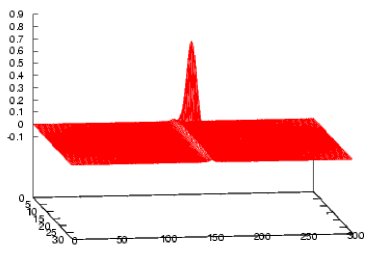
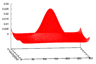
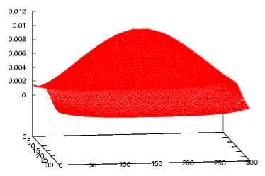
In Fig. 2 we show some examples of the real probability distribution at large Langevin time for various and a given cutoff . The direction goes from left to right and the compact direction from back to front. We observe that at small , the distribution resembles the analytic result at . The distribution is very narrow in the direction and boundary effects are not expected to play a role. Increasing results in a wider distribution, and boundary effects become clearly visible. The apparent non-smooth behaviour at the edge is to be expected from the discontinuity across the seam, discussed at the end of the previous section.
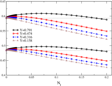
After obtaining the distribution, expectation values of observables follow from Eq. (22). In Tables 1 – 7 (see end of paper) we compare the results of the Langevin simulation and the FPE for increasing values of from up to . Note that the Langevin equation can be solved without a cutoff (). The imaginary parts of the observables are consistent with zero. The data of the tables are also summarized in Figs. 3, 4 (the FPE and the CLE data are indistinguishable at the scale of the figures; the rightmost points in Fig. 4 correspond to for FPE and for CLE).

The following facts can be inferred from these results:
(1) CLE and FPE give rather similar results, but sometimes they differ by
several (statistical error of the CLE simulation).
(2) All the data show a clear dependence on , in contrast to the
conclusion of the formal arguments. For larger values both CLE and
FPE give results different from the exact values.
(3) The best results are generally obtained for the smallest . In
this case there is also the weakest dependence, in fact no
dependence whatsoever for .
Obviously the presence of the cutoff and periodic boundary conditions affects the CLE and FPE in a similar way. But the dependence shows the failure of the formal argument, even for . At least for one has a clear case of ‘convergence to a wrong limit’. The data of the CLE with and are actually not really converged, except for Observing the scatter plots for different Langevin times it appears unclear whether the observables really reach an equilibrium distribution – they tend to drift out to infinity, whereas their averages, while remaining small, suffer from huge fluctuations. On the other hand the observables seem to reach a stable distribution for and any .
V.2 The model of Guralnik and Pehlevan
Guralnik and Pehlevan guralnik studied an instructive toy model on and , called GP model henceforth. Its action is
| (68) |
and was studied in connection with PT invariant but non-hermitian Hamiltionians (where PT indicates the combined action of parity and time reversal) bender .
The action (68) leads to the drift forces
| (69) |
There is a stable fixed point at and an unstable one at . The ‘classical trajectories’ obtained by leaving out the noise are given by
| (70) |
Since this is a Möbius transformation from to the trajectories are circles. They can be imagined to emerge from the unstable fixed point at and go to the stable fixed point as . Those classical trajectories again can be seen clearly in the large excursions, since there the noise becomes negligible. Fig. 6 shows the result from a Langevin simulation at and (in this case there are 50000 update steps between two consecutive points).


Guralnik and Pehlevan give the exact results of the first three moments at , they are
| (71) |
They solved the discretized Langevin equation numerically, using , and obtained good agreement with those exact results. We did some more and probably longer simulations at , , , . The results for are shown in Fig. 6; again they show a clear dependence on , in conflict with the formal reasoning. While for small there is agreement with the exact result, for larger we again have convergence to the wrong limit.


The results for show a similar behaviour, except that at the result is , with a statistical error that is huge compared to the error found at . The data for show an even more dramatic failure for larger : they diverge for , whereas for fluctuations are large. Finally we measured , which has an exact value of . Here divergence becomes manifest already for (but it might occur for all ).
In order to have an idea of the equilibrium distribution for we show in Fig. 7 a scatter plot of 50000 configurations in the complex plane. Non-Gaussian behaviour is quite clear from this plot. Noticeable is the appearance of sharp edges of the distribution, possibly indicating jumps, but no functions like in the case in the hopping expansion. To obtain these pictures we sampled over 60000 points taken at equal intervals of 0.5 in Langevin time. Similar distributions have been observed in Ref. aartsstam for the full U(1) one-link model. The non-Gaussian character is further demonstrated in Fig. 8: the histograms for both and deviate strongly from a Gaussian distribution.
VI Tentative conclusions
VI.1 Explanation of wrong results
We will now try to interpret these findings. They are quite analogous in the two model cases and we will try to reach some conclusions that can be generalized to more realistic models.
The question of convergence vs. divergence apparently depends on the values of , but it is more plausible that there is no qualitative difference between the different positive values of , only the time needed to observe the asymptotic behaviour is different. On the other hand for there seems to be really a qualitative difference: the distributions develop discontinuities or even functions; but more important is the fact that they seem to drop very rapidly in the imaginary direction.
We tentatively conclude that for the systems relax to equilibrium measures that show at least exponential decay in imaginary direction (in our simple model this decay is of course much stronger – the measure is zero for ).
For the situation is less clear, but it seems that in the model we get a decay at least like , but probably not stronger than any exponential. In the model of Guralnik and Pehlevan the data suggest a power-like decay (the power appears to be near 2).
To sum up our tentative conclusions:
There is a unique equilibrium distribution for the Langevin processes for any , but for it shows limited decay, especially in the imaginary direction.
The type of decay for depends on the model considered; but for some observables their growth in imaginary direction may conspire with the falloff of the equilibrium measure in such a way that we obtain convergence to a wrong limit. In any case one should not expect convergence of the mean value for all holomorphic observables.
For very small and limited simulation time, the behaviour is of course indistinguishable from the one at , and one may reach a quasi-convergence to the right limit, even if an infinitely long simulation would diverge.
If we try to generalize boldly from our toy model to real lattice gauge theories, we expect that for and for most interesting observables, such as Wilson loops, Polyakov loops etc., we have to expect boundary terms contributing even as the boundary is sent to infinity. For multiply charged loops and the situation could be even worse: those boundary contributions may diverge as the boundary is moved to infinity. But these problems probably will not occur for and do not show up at very small values of either, at least if simulations are not run excessively long.
We realize that definite conclusions about the falloff of the probability density in the direction have not yet been reached; we intend to return to a more detailed study of this question in a future paper.
VI.2 Practical conclusions
The conclusions for practical applications are quite straightforward:
(1) In complex Langevin simulations one should use . If one wants to do a random walk simulation or an iterate of the Fokker-Planck operator, this is not possible, but one should make sure that .
(2) Always validate the simulations by comparison with other trusted computations for parameter values where other methods are available.
(3) Wilson or Polyakov loops of higher charge will generally have much larger fluctuations. In general they are not needed for physics applications, but they may be worth looking at because they can give information about the probability distribution.
Acknowledgements.
We thank Frank James and Denes Sexty for discussion. I.-O.S. thanks the MPI for Physics München and Swansea University for hospitality. G.A. is supported by STFC.References
- (1) J. Klauder, Acta Phys. Austriaca Suppl. XXXV (1983) 251; J. Phys. A: Math. Gen. 16, L317-319 (1983); Phys. Rev. A 29, 2036-2047 (1984).
- (2) G. Parisi, Phys. Lett. 131 B (1983) 393.
- (3) F. Karsch and H. W. Wyld, Phys. Rev. Lett. 55 (1985) 2242.
- (4) P. H. Damgaard and H. Hüffel, Phys. Rept. 152 (1987) 227.
- (5) J. Ambjorn and S. K. Yang, Phys. Lett. B 165, 140 (1985).
- (6) J. Klauder and W. P. Petersen, J. Statist. Phys. 39 (1985) 53.
- (7) H. Q. Lin and J. E. Hirsch, Phys. Rev. B 34 (1986) 1964.
- (8) J. Ambjorn, M. Flensburg and C. Peterson, Nucl. Phys. B 275, 375 (1986).
- (9) J. Berges and I. O. Stamatescu, Phys. Rev. Lett. 95 (2005) 202003 [hep-lat/0508030].
- (10) J. Berges, S. Borsanyi, D. Sexty and I. O. Stamatescu, Phys. Rev. D 75 (2007) 045007 [hep-lat/0609058].
- (11) J. Berges and D. Sexty, Nucl. Phys. B 799, 306 (2008) [0708.0779 [hep-lat]].
- (12) G. Aarts and I. O. Stamatescu, JHEP 0809 (2008) 018 [0807.1597 [hep-lat]].
- (13) G. Aarts, Phys. Rev. Lett. 102 (2009) 131601 [0810.2089 [hep-lat]].
- (14) G. Aarts, JHEP 0905 (2009) 052 [0902.4686 [hep-lat]].
- (15) C. Pehlevan and G. Guralnik, Nucl. Phys. B 811, 519 (2009) [0710.3756 [hep-th]].
- (16) G. Guralnik and C. Pehlevan, Nucl. Phys. B 822, 349 (2009) [0902.1503 [hep-lat]].
- (17) G. Aarts, F. James, E. Seiler and I. O. Stamatescu, Phys. Lett. B (to appear) [arXiv:0912.0617 [hep-lat]].
- (18) G. G. Batrouni, G. R. Katz, A. S. Kronfeld, G. P. Lepage, B. Svetitsky and K. G. Wilson, Phys. Rev. D 32 (1985) 2736.
- (19) H. Gausterer and H. Thaler, J. Phys. A: Math. Gen. 31 (1998) 2541.
- (20) H. Gausterer, Nucl. Phys. A642 (1998) 239c.
- (21) R. C. Gunning and H. Rossi, Analytic Functions of Several Complex Variables, Prentice-Hall, Englewood Cliffs, N.J. 1965.
- (22) V. S. Valdimirov, Methods of the Theory of Functions of Many Complex Variables, MIT Press, Cambridge, Mass. 1966.
- (23) E. B. Davies, Linear Operators and their Spectra, Cambridge University Press, Cambridge, UK 2007.
- (24) B. Helffer and F. Nier, Hypoelliptoc Estimates and Spectral Theory for Fokker-Planck Operators and Witten Laplacians, Springer, Berlin, Germany 2005.
- (25) D. Gilbarg and N. S. Trudinger, Elliptic Partial Differential Equations of Second Order, Springer, Berlin et al 1977.
- (26) C. M. Bender, Rept. Prog. Phys. 70 (2007) 947 [hep-th/0703096].
| 0.032 | CLE | 0.48331(047) | 0.59265(058) | 0.12311(037) | 0.19865(055) |
|---|---|---|---|---|---|
| 0.158 | CLE | 0.48331(047) | 0.59265(058) | 0.13211(037) | 0.19865(055) |
| 0.474 | CLE | 0.48331(047) | 0.59265(058) | 0.13211(037) | 0.19865(055) |
| 0.790 | CLE | 0.48331(047) | 0.59265(058) | 0.13211(037) | 0.19865(055) |
| 1.581 | CLE | 0.48331(047) | 0.59265(058) | 0.13211(037) | 0.19865(055) |
| CLE | 0.48331(047) | 0.59265(058) | 0.13211(037) | 0.19865(055) | |
| exact | 0.48356 | 0.59297 | 0.13065 | 0.19646 |
| 0.032 | CLE | 0.48344(046) | 0.59281(057) | 0.13154(036) | 0.19778(054) |
|---|---|---|---|---|---|
| FPE | 0.48358 | 0.59297 | 0.13065 | 0.19646 | |
| 0.158 | CLE | 0.48369(047) | 0.59313(057) | 0.13194(036) | 0.19835(055) |
| FPE | 0.48361 | 0.59302 | 0.13065 | 0.19645 | |
| 0.474 | CLE | 0.48370(047) | 0.59313(058) | 0.13188(036) | 0.19822(054) |
| FPE | 0.48376 | 0.59307 | 0.13066 | 0.19639 | |
| 0.790 | CLE | 0.48372(048) | 0.59319(059) | 0.13186(036) | 0.19812(055) |
| FPE | 0.48405 | 0.59292 | 0.13076 | 0.19618 | |
| 1.581 | CLE | 0.48382(047) | 0.59330(058) | 0.13183(037) | 0.19792(056) |
| FPE | 0.48647 | 0.59033 | 0.13318 | 0.19449 | |
| CLE | 0.48396(047) | 0.59345(058) | 0.13089(042) | 0.19685(056) | |
| exact | 0.48356 | 0.59297 | 0.13065 | 0.19646 |
| 0.032 | CLE | 0.48345(050) | 0.59280(062) | 0.13114(035) | 0.19714(052) |
|---|---|---|---|---|---|
| FPE | 0.48366 | 0.59290 | 0.13066 | 0.19646 | |
| 0.158 | CLE | 0.48385(054) | 0.59335(067) | 0.13153(039) | 0.19771(059) |
| FPE | 0.48371 | 0.59313 | 0.13064 | 0.19644 | |
| 0.474 | CLE | 0.48402(052) | 0.59357(064) | 0.13148(037) | 0.19762(056) |
| FPE | 0.48399 | 0.59348 | 0.13059 | 0.19637 | |
| 0.790 | CLE | 0.48425(053) | 0.59377(065) | 0.13146(038) | 0.19764(057) |
| FPE | 0.48425 | 0.59379 | 0.13056 | 0.19627 | |
| 1.581 | CLE | 0.48485(051) | 0.59454(063) | 0.13115(036) | 0.19725(054) |
| FPE | 0.48476 | 0.59437 | 0.12363 | 0.19583 | |
| CLE | 0.48527(051) | 0.59504(063) | 0.12944(047) | 0.19387(079) | |
| exact | 0.48356 | 0.59297 | 0.13065 | 0.19646 |
| 0.032 | CLE | 0.48342(049) | 0.59293(060) | 0.13095(038) | 0.19692(057) |
|---|---|---|---|---|---|
| FPE | 0.48373 | 0.59226 | 0.13074 | 0.19602 | |
| 0.158 | CLE | 0.48410(051) | 0.59346(062) | 0.13068(037) | 0.19632(056) |
| FPE | 0.48399 | 0.59344 | 0.13065 | 0.19647 | |
| 0.474 | CLE | 0.48538(051) | 0.59497(064) | 0.13090(038) | 0.19702(058) |
| FPE | 0.48488 | 0.59457 | 0.13050 | 0.19623 | |
| 0.790 | CLE | 0.48619(051) | 0.59605(061) | 0.13066(041) | 0.19655(063) |
| FPE | 0.48572 | 0.59559 | 0.13027 | 0.19589 | |
| 1.581 | CLE | 0.48762(052) | 0.59761(062) | 0.12934(044) | 0.19503(064) |
| FPE | 0.48729 | 0.59753 | 0.12934 | 0.19449 | |
| CLE | 0.48890(050) | 0.59942(063) | 0.12392(068) | 0.18602(086) | |
| exact | 0.48356 | 0.59297 | 0.13065 | 0.19646 |
| 0.032 | CLE | 0.48047(049) | 0.58917(060) | 0.12935(035) | 0.19450(053) |
|---|---|---|---|---|---|
| FPE | 0.48073 | 0.58856 | 0.12894 | 0.19328 | |
| 0.158 | CLE | 0.48240(051) | 0.59150(063) | 0.13039(037) | 0.19613(056) |
| FPE | 0.48313 | 0.59163 | 0.13055 | 0.19584 | |
| 0.474 | CLE | 0.48747(053) | 0.59753(067) | 0.13080(041) | 0.19645(059) |
| FPE | 0.48739 | 0.59760 | 0.13064 | 0.19646 | |
| 0.790 | CLE | 0.49012(055) | 0.60078(069) | 0.12952(045) | 0.19437(069) |
| FPE | 0.49020 | 0.60107 | 0.12984 | 0.19525 | |
| 1.581 | CLE | 0.49532(052) | 0.60714(068) | 0.12647(054) | 0.19056(085) |
| FPE | 0.49550 | 0.60758 | 0.12668 | 0.19051 | |
| CLE | 0.49995(049) | 0.61287(063) | 0.10733(202) | 0.16132(376) | |
| exact | 0.48356 | 0.59297 | 0.13065 | 0.19646 |
| 0.032 | CLE | 0.46720(051) | 0.57290(063) | 0.12150(034) | 0.18269(051) |
|---|---|---|---|---|---|
| FPE | 0.46763 | 0.57253 | 0.12118 | 0.18165 | |
| 0.158 | CLE | 0.46985(054) | 0.57620(066) | 0.12335(037) | 0.18557(055) |
| FPE | 0.47070 | 0.57629 | 0.12363 | 0.18533 | |
| 0.474 | CLE | 0.48570(057) | 0.59533(071) | 0.13167(042) | 0.19766(065) |
| FPE | 0.48608 | 0.59542 | 0.13184 | 0.19793 | |
| 0.790 | CLE | 0.49664(055) | 0.60871(068) | 0.13166(046) | 0.19731(074) |
| FPE | 0.49644 | 0.60858 | 0.13166 | 0.19799 | |
| 1.581 | CLE | 0.51104(056) | 0.62580(080) | 0.12366(074) | 0.18370(114) |
| FPE | 0.51055 | 0.62601 | 0.12363 | 0.18595 | |
| CLE | 0.52272(051) | 0.64013(069) | 0.07553(204) | 0.11359(334) | |
| exact | 0.48356 | 0.59297 | 0.13065 | 0.19646 |
| 0.032 | CLE | 0.45144(051) | 0.55358(062) | 0.11267(035) | 0.16941(053) |
|---|---|---|---|---|---|
| FPE | 0.45203 | 0.55343 | 0.11236 | 0.16843 | |
| 0.158 | CLE | 0.45456(055) | 0.55742(067) | 0.11453(038) | 0.17224(054) |
| FPE | 0.45513 | 0.55722 | 0.11479 | 0.17207 | |
| 0.474 | CLE | 0.47443(057) | 0.58151(071) | 0.12738(044) | 0.19117(065) |
| FPE | 0.47501 | 0.58165 | 0.12759 | 0.19136 | |
| 0.790 | CLE | 0.49560(053) | 0.60668(073) | 0.13448(052) | 0.20120(081) |
| FPE | 0.49575 | 0.60740 | 0.13446 | 0.20198 | |
| 1.581 | CLE | 0.52141(093) | 0.63883(093) | 0.12345(098) | 0.18569(144) |
| FPE | 0.52157 | 0.63948 | 0.12426 | 0.18692 | |
| CLE | 0.54104(059) | 0.66230(082) | 0.05049(354) | 0.07723(522) | |
| exact | 0.48356 | 0.59297 | 0.13065 | 0.19646 |