Conducting-angle-based percolation in the XY model

Abstract

We define a percolation problem on the basis of spin configurations of the two dimensional XY model. Neighboring spins belong to the same percolation cluster if their orientations differ less than a certain threshold called the conducting angle. The percolation properties of this model are studied by means of Monte Carlo simulations and a finite-size scaling analysis. Our simulations show the existence of percolation transitions when the conducting angle is varied, and we determine the transition point for several values of the XY coupling. It appears that the critical behavior of this percolation model can be well described by the standard percolation theory. The critical exponents of the percolation transitions, as determined by finite-size scaling, agree with the universality class of the two-dimensional percolation model on a uniform substrate. This holds over the whole temperature range, even in the low-temperature phase where the XY substrate is critical in the sense that it displays algebraic decay of correlations.

I Introduction

Consider the XY or planar model on the square lattice with periodic boundary conditions, described by the reduced Hamiltonian

$${\mathcal{H}}=-\frac{J}{k_{\rm B}T}\sum_{<ij>}\vec{s}_{i}\cdot\vec{s}_{j},$$ (1)

where the sum is over all nearest-neighbor pairs, and the $\vec{s}_{i}$ are two-dimensional unit vectors labeled by the site number $i$. We restrict the nearest-neighbor interaction to be ferromagnetic, i.e., $J>0$.

When the temperature of this model is lowered, it undergoes a phase transition of an interesting character, which was explained by Kosterlitz and Thouless KT . More exact results for the exponents were obtained by Nienhuis Nhon for an O(2) model in the same universality class. These results show that the renormalization exponent $y_{t}$ of the temperature is equal to 0, which means that the temperature-driven transition is of infinite order, i.e. the specific-heat singularity is extremely weak. In contrast, the magnetic susceptibility displays a very strong divergence when the temperature is lowered to the transition point.

At temperatures $T>0$ below the transition point there is no spontaneous long-range order in the sense that the magnetization is zero MW . Instead, the low-temperature phase resembles a critical state; the correlations decay algebraically, with exponents that are still dependent on the temperature.

Recently, there has been ample attention to percolation problems defined on a critical substrate, see e.g. Refs. XYH, ; DBN, ; DDGQB, ; DDGB, and references therein. It thus appears that, for Potts and O($n$) models, the universal properties of such percolation transitions do reflect the nature of the critical substrate. These investigations are based on model representations with discrete degrees of freedom.

It is thus interesting to investigate related problems using a substrate with continuous degrees of freedom. For instance, the mechanical properties of static granular matter can be analyzed in terms of the so-called force networks GHM ; JNB . By introducing a threshold force, such that forces exceeding the threshold form clusters, a percolation transition is seen at a critical force threshold. This approach was applied to different models for granular piles, that are expected to belong to different universality classes. It was found that also the corresponding percolation behavior could discriminate between the different models OSN . This might suggest that such substrate dependence is a general phenomenon for critical models with continuous degrees of freedom, i.e., the critical behavior of the percolation clusters might generally reflect the long-range correlations of the original degrees of freedom.

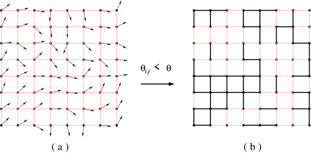
In order to shed more light on this issue, the present work investigates a percolation problem using the substrate of the two-dimensional XY-model. In particular we are interested how the universal properties of the percolation transition will depend on the temperature of the underlying XY model. We define the percolation problem such as to depend only on the XY configuration, and not on any additional random variables. This is achieved by introducing a “conducting angle” $\theta$ such that neighboring spins whose orientations differ by less than $\theta$ are connected by a percolation bond. This name is based on the analogy with a conductance problem of conducting units on a lattice, such that neighboring units are in electrical contact only if their orientations match to a sufficient degree.

It is clear that this conducting angle also defines a threshold pair energy, below which a pair of neighboring XY spins is connected by a percolation bond. These percolation bonds define a bond percolation configuration involving a complete decomposition of the lattice in percolation clusters. An example of an XY configuration with the corresponding percolation cluster decomposition is shown in Fig. 1.

Figure 1: Construction of a bond-percolation configuration (b) from an XY spin configuration (a). If the angle $\theta_{ij}$ between a pair (i, j) of neighboring spins is less than a given angle $\theta$, the neighboring spins are connected by a bond, so that the lattice decomposes into a system of percolation clusters. The threshold was chosen as $\theta=\pi/6$ in this figure.

It is obvious that the resulting bond percolation configurations will not percolate for $\theta=0$, and that they will percolate for $\theta=\pi$ and larger. We are thus left with the task to find the percolation threshold $\theta_{\rm c}$ and the critical exponents as a function of the temperature. To answer these questions, we perform simulations of the two-dimensional (2D) XY spin model, which are described in Section II. Section III presents the numerical results, including the critical parameters. We include a short discussion in Sec. IV.

II Algorithm

For reasons of efficiency, we make use of a cluster algorithm SW to simulate the XY model. We applied the single-cluster algorithm formulated by Wolff W2 to the model on the square lattice. We recall the steps involved in one Wolff cluster flip:

1. Choose an arbitrary direction as the $y$-direction, and denote by $\alpha_{i}$ the angle between the spin $\vec{s_{i}}$ and the $y$-axis. Define an Ising spin $s_{i}=\pm 1$ with the same sign as the $y$-component of $\vec{s_{i}}$. Thus, the nearest-neighbor interaction term in ${\mathcal{H}}_{ij}$ between spins $i$ and $j$ reads

   $${\mathcal{H}}_{ij}=-K\vec{s}_{i}\cdot\vec{s}_{j}=-Ks_{i}^{x}s_{j}^{x}-Ks_{i}^{y}s_{j}^{y}=-Ks_{i}^{x}s_{j}^{x}-K\cos(\alpha_{i})\cos(\alpha_{j})\,s_{i}s_{j}\,,$$ (2)

   where $K\equiv J/k_{\rm B}T$. As far as the dependence of ${\mathcal{H}}_{ij}$ on the Ising variables ${s_{i}}$ and ${s_{j}}$ is concerned, this is an Ising coupling between the two spins with strength $K_{ij}=K\cos\alpha_{i}\cos\alpha_{j}$. One may update the Ising variables using a cluster algorithm that takes into account these position-dependent couplings. The following steps are used to update the $y$-components of the spins.

2. Choose a spin randomly, say on site $i$. For each nearest-neighbor site $j$ of $i$, connect $i$ and $j$ by a bond with probability $p_{ij}=\max(0,1-e^{-2K_{ij}})$. Then do the same for each of the nearest-neighbor sites of each newly connected site, and so on. The process continues until no more new sites are connected. Then, the construction of the cluster, which contains all sites connected via some path of bonds to site $i$, is finished.

3. Change the sign of the $y$-components of all spins in that cluster.

III Numerical results and analysis

During the simulations, we constructed percolation cluster decompositions on the basis of a chosen conducting angle $\theta$. For each such decomposition we sampled several quantities in order to estimate the second moment of the cluster size distribution $S_{2}$, the probability $P$ that there exists a cluster that wraps the system, a dimensionless ratio $Q$ that can be related to the Binder cumulant, and the cluster size distribution function $n_{s}$. We shall proceed to introduce these quantities in more detail and list their expected finite-size scaling properties.

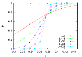
Since we are using finite systems with periodic boundary conditions, we define a ”wrapping cluster” Pinson as a percolation cluster that connects to itself along at least one of the periodic directions. For each XY configuration $S$ we thus define a quantity $p(S,\theta)$ that has the value 1 if there exists a wrapping cluster, and $p(S,\theta)=0$ otherwise. Thus, for a system with finite size $L$, the probability $P(K,\theta,L)$ that a wrapping cluster exists is given by

$$P(K,\theta,L)=\langle p(S,\theta)\rangle\,,$$ (3)

where the ensemble average is taken for an XY system with linear size $L$ and coupling $K$. If there is a percolation transition at a conducting angle $\theta_{\rm c}$, one expects that $\theta$ plays the role of a temperature-like variable, and thus that the finite-size scaling behavior FSS of $P$ is described by

$$P(K,\theta,L)=P^{(c)}+a(\theta-\theta_{\rm c})L^{y_{{}_{p}}}+\cdots+b_{1}L^{y_{{}_{1}}}+b_{2}L^{y_{{}_{2}}}+\cdots,$$ (4)

where $y_{p}$ controls the scaling of $\theta$ and acts as a temperature-like exponent, corresponding with the bond dilution exponent in the language of the percolation model. The exponents $y_{1}$, $y_{2}$, etc. are correction-to-scaling exponents, which are unknown in principle. The constant $P^{(c)}$, which is defined as the value of $P$ at $\theta_{\rm c}$ in the limit $L\to\infty$, and the exponent $y_{p}$ are universal, but the universality class of the present percolation problem remains to be determined.

The second moment $S_{2}$ of the percolation cluster size distribution can also be viewed as the mean size of the cluster containing an arbitrary point. It is defined as

$$S_{2}=\frac{1}{N^{2}}\left<\sum_{i}^{N_{c}}s_{i}^{2}\right>\,,$$ (5)

where $s_{i}$ is the size of the $i$-th cluster, $N_{c}$ the total number of clusters for a configuration, and $N=L^{2}$ is the volume of the system. The quantity $S_{2}$ is also closely related with the generalization $\chi_{\rm RC}$ of the $q$-state Potts magnetic susceptibility to the random-cluster model, applied to the special case $q=1$. This relation is expressed as $\chi_{\rm RC}=NS_{2}$.

In analogy with the Potts susceptibility, we expect the following finite-size-scaling behavior for $S_{2}$ in the neighborhood of a percolation threshold at $\theta_{\rm c}$:

$$S_{2} = L^{2y_{{}_{h}}-2d}[a_{0}+a_{1}(\theta-\theta_{\rm c})L^{y_{{}_{p}}}+\cdots+b_{1}L^{y_{{}_{1}}}+b_{2}L^{y_{{}_{2}}}+\cdots]\,,$$ (6)

where $y_{h}$ is the fractal dimension of critical percolation clusters. At the percolation threshold $\theta_{\rm c}$, this equation reduces to

$$S_{2} = L^{2y_{{}_{h}}-2d}(a_{0}+b_{1}L^{y_{{}_{1}}}+b_{2}L^{y_{{}_{2}}}+\cdots)\,.$$ (7)

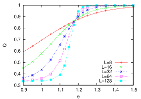
We also define a dimensionless ratio related to the Binder cumulant Binder as

$$Q=\frac{S_{2}^{2}}{3S_{2}^{(2)}-2S_{4}}\,,$$ (8)

where $S_{2}^{(2)}$ is defined as

$$S_{2}^{(2)}=\frac{1}{N^{4}}\left<\left(\sum_{i}^{N_{c}}s_{i}^{2}\right)^{2}\right>,$$ (9)

and $S_{4}$ as

$$S_{4}=\frac{1}{N^{4}}\left<\sum_{i}^{N_{c}}s_{i}^{4}\right>\,.$$ (10)

The relation with the Binder cumulant is based on the fact that Eq. (8) is obtained when the Binder ratio $\langle m^{2}\rangle^{2}/\langle m^{4}\rangle$ of magnetization moments of the Ising model is expressed in the language of the $q=2$ random-cluster model. In analogy with the Binder cumulant, we expect that, in the neighborhood of the percolation threshold, it behaves like

$$Q(K,\theta,L)=Q^{(c)}+a_{1}(\theta-\theta_{\rm c})L^{y_{p}}+\cdots+b_{1}L^{y_{{}_{1}}}+b_{2}L^{y_{{}_{2}}}+\cdots\,.$$ (11)

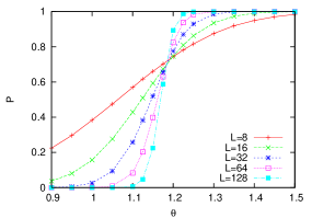
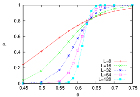
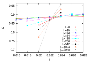
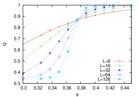
III.1 Wrapping probability as a function of $\theta$

We simulated XY systems with linear sizes $L=8$, 16, 32, 64, 128, and 256 at different inverse temperatures: $K=0$, 0.001, 0.01, 0.10, $\cdots$, 5.00, and 10.00. For $K=0.9$ and $K=1.0$, system sizes up to $L=1024$ and $2048$ were simulated respectively. Typically, $10^{7}$ XY configurations were sampled. The samples were taken at intervals consisting of one Metropolis sweep and four Wolff clusters. For each of these XY configurations, percolation cluster decompositions were constructed with several different values of the conducting angle.

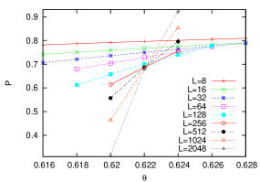
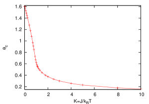
Some results for the wrapping probability $P(K,\theta,L)$ as a function of the conducting angle are shown in Figs. 2-4. These figures show clear intersections corresponding with percolation thresholds. Furthermore, the behavior appears to be remarkably similar for different values of the XY coupling $K$. We applied the least-squares method to fit the wrapping probability by the finite-size-scaling equation (4). The results for the percolation threshold $\theta_{\rm c}$ are shown in Fig. 5 as a function of the XY coupling $K$. They are also included in Table 1 for each value of $K$, together with the results for the exponent $y_{p}$ and the universal probability $P^{(c)}$. The results for the latter quantity reproduce, within error bounds, the literature value $P^{(c)}=0.690473725$ which applies to the ordinary two-dimensional percolation model Pinson ; ZLK ; NZ .

Figure 2: (color online). Wrapping probability versus $\theta$ at $K=0.5$. The curves are added as a guide for the eye.

Figure 3: (color online). Wrapping probability versus $\theta$ at $K=1$. The right-hand figure shows the details in the vicinity of $\theta_{\rm c}$, where the finite size effect becomes relatively strong. The curves are added as a guide for the eye.

Figure 4: (color online). Wrapping probability versus $\theta$ at $K=2.0$. The curves are added as a guide for the eye.

Figure 5: Percolation threshold $\theta_{\rm c}$ versus $K$. For $K=0$, the critical value of the conducting angle is 1.61078 radians or about 92 degrees. This value applies to a system of randomly oriented conductors on the square lattice. The curve is added as a guide for the eye, and estimated error bars are smaller than the size of the symbols.

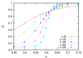
III.2 Dimensionless ratio $Q$ as a function of $\theta$

We also sampled the ratio $Q$ for systems at different inverse temperatures. Some of the data are shown in Figs. 6 to 8. They display the same general behavior as the wrapping probability in the preceding subsection.

A least-squares analysis of the data for $Q(K,\theta,L)$ on the basis of the finite-size-scaling equation (11) results in the estimates of $y_{p}$, $Q^{(c)}$, and the percolation threshold $\theta_{\rm c}$. The estimates of $y_{p}$ and $\theta_{\rm c}$ are in agreement with those found by fitting $P(K,\theta,L)$. The estimates of the universal value $Q^{(c)}$ are also listed in Table 1 for each $K$. Their values are in agreement with the literature value DB $0.87053~{}(2)$ for the ordinary two-dimensional percolation model.

Figure 6: (color online). Dimensionless ratio $Q$ versus conducting angle $\theta$ for $K=0.5$. The curves are added as a guide for the eye.

Figure 7: (color online). Dimensionless ratio $Q$ versus conducting angle $\theta$ for $K=1.0$. The right-hand figure shows the details in the vicinity of $\theta_{\rm c}$. The curves are added as a guide for the eye.

Figure 8: (color online). Dimensionless ratio $Q$ versus conducting angle $\theta$ for $K=2.0$. The curves are added as a guide for the eye.

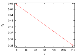
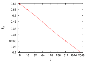
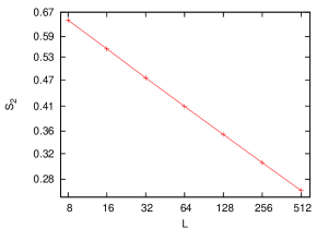
III.3 The second moment $S_{2}$ at the percolation threshold

We simulated the model with system sizes $L=8$, 16, 32, 64, 128, 256 and $512$ at the estimated percolation threshold $\theta_{\rm c}$ for each $K$, and sampled the second moment $S_{2}$ of the cluster-size distribution. Samples were taken at intervals consisting of one Metropolis sweep and four Wolff clusters. The numbers of samples taken for system sizes $L=8$ to $32$, $L=64$ to $128$, and $L=256$ to $512$ are $10^{7}$, $4\times 10^{6}$ and $2\times 10^{6}$ respectively. For $K=1.0$, which is in the vicinity of the Kosterlitz-Thouless (KT) transition, additional simulations took place for system sizes $L=1024$ and 2048, involving several times $10^{6}$ samples per system size.

Some of the data for $S_{2}$ are shown as a function of the system size $L$ in Figs. 9-11 for some values of $K$. These figures use logarithmic scales, so that linear behavior means that $S_{2}$ behaves as a power of $L$, in accordance with criticality. For $K=1.0$, which is close to the KT transitions, small deviations from linearity are visible.

Figure 9: Second moment $S_{2}$ of the cluster size distribution versus finite size $L$, for XY coupling $K=0.5$. The curve is added as a guide for the eye, and estimated error bars are smaller than the size of the symbols.

Figure 10: Second moment $S_{2}$ of the cluster size distribution versus finite size $L$, for XY coupling $K=1.0$. The curve is added as a guide for the eye, and estimated error bars are smaller than the size of the symbols.

Figure 11: Second moment $S_{2}$ of the cluster size distribution versus finite size $L$, for XY coupling $K=2.0$. The curve is added as a guide for the eye, and estimated error bars are smaller than the size of the symbols.

We fitted $S_{2}$ by the finite-size-scaling formula Eq. (7), and thus obtained estimates of the fractal dimension $y_{h}$, which are listed in Table 1 for several values of $K$. For $K=1.0$, a satisfactory fit could only be obtained by discarding system sizes $L<128$ and including system sizes up to $L=2048$.

III.4 The distribution $n_{s}$ of the cluster size $s$

At the percolation transition $\theta_{\rm c}$, the requirement that the cluster size distribution scales in a covariant way yields a power law for this distribution

$$n_{s}(s,\theta_{\rm c})\propto s^{-\tau}\,,$$ (12)

where $\tau$ is a critical exponent equal to $1+d/y_{h}$, with $d=2$ dimensions and the fractal dimension $y_{h}$ of the percolation clusters. For the ordinary $d=2$ percolation model, one has $y_{h}=91/48$ CG ; Cardy , and thus $\tau=187/91$.

Parts of the data for $n_{s}$ are shown in Figs. 12-14 as a function of cluster size $s$, for different values of the XY coupling $K$.

Figure 12: (color online). Cluster size distribution function as a function of cluster size $s$ for $K=0.5$, $\theta_{\rm c}=1.18179$.

Figure 13: (color online). Cluster size distribution function as a function of cluster size $s$ for $K=1.0$, $\theta_{\rm c}=0.62210$.

Figure 14: (color online). Cluster size distribution function as a function of cluster size $s$ for $K=2.0$, $\theta_{\rm c}=0.37560$.

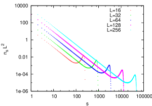
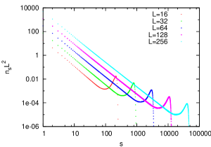
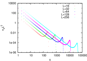
The axes in these figures use logarithmic scales. The data points are, in a wide range of cluster sizes, well approximated by straight lines, corresponding with a scale-invariant distribution according to a power law. The slopes of these lines are close to the value of $\tau$ that applies to the ordinary percolation model. The curves in Figs. 12-14 can obviously be brought to an approximate data collapse by introducing suitable prefactors, but it appears that there is still an appreciable finite-size dependence.

For a numerical determination of $\tau$ from the data for $n_{s}$, we use a least-squares analysis of the range of $s$ where $n_{s}$ is almost linear in Figs. 12-14, thus excluding small clusters smaller than 20, and the largest clusters exceeding a size $L^{y_{h}}/10$. Even then, two correction terms had to be included in order to obtain satisfactory residuals, according to the fit formula

$$n_{s}(s,\theta_{\rm c},L)=a_{0}s^{-\tau}(1+a_{1}s^{y_{1}}+a_{2}L^{y_{2}})\,,$$ (13)

where the term with coefficient $a_{2}$ is significant only for $K>1$. Satisfactory fits were obtained for all inverse temperatures. For example, for $K=0.75$, we fitted the data simultaneously for system sizes $L=32$, 64,$\cdots$, 512 using the above formula, and found $\tau=2.055~{}(2)$, $y_{1}=-0.57~{}(1)$ with $\chi^{2}$ per degree of freedom almost equal to 1. For $K=2.0$, a fit of the data for system sizes $L=32$,64,$\cdots$, 512 yielded $\tau=2.054~{}(2)$, $y_{1}=-1.0~{}(1),y_{2}=-1.6~{}(1)$, again with a satisfactory value of $\chi^{2}$ as compared with the number of degrees of freedom.

We thus obtained estimates of the exponent $\tau$ that agree well with the value $\tau=187/91=2.0549\cdots$ for the ordinary 2D percolation model, for several temperatures of the XY model.

Table 1: Numerical results for the percolation threshold $\theta_{\rm c}$, the bond dilution exponent $y_{p}$, the fractal dimension $y_{h}$, the universal wrapping probability $P^{(c)}$ and the universal dimensionless ratio $Q^{(c)}$. The exact values for two-dimensional percolation exponents are $y_{p}=3/4$ and $y_{h}=91/48=1.895833\cdots$.

$K$	$\theta_{\rm c}$	$y_{p}$	$y_{h}$	$P^{(c)}$	$Q^{(c)}$
0	1.61078 (2)	0.750(2)	1.8961 (3)	0.6906 (2)	0.8708 (3)
0.001	1.60994 (2)	0.748(3)	1.8961 (3)	0.6908 (3)	0.8707 (5)
0.010	1.60252 (2)	0.750(2)	1.8959 (3)	0.6905 (3)	0.8706 (3)
0.100	1.52866 (2)	0.751(2)	1.8959 (3)	0.6905 (3)	0.8708 (5)
0.200	1.44651 (2)	0.752(2)	1.8958 (3)	0.6903 (4)	0.8708 (5)
0.500	1.18179 (2)	0.750(2)	1.8956 (3)	0.6903 (3)	0.8709 (5)
0.750	0.91074 (2)	0.751(2)	1.8957 (3)	0.6901 (5)	0.8704 (5)
0.800	0.85002 (2)	0.749(5)	1.8957 (3)	0.6905 (3)	0.8702 (5)
0.900	0.72804 (2)	0.751(4)	1.8958 (3)	0.6902 (4)	0.8705 (5)
1.000	0.62209 (2)	0.74 (2)	1.894  (2)	0.6907 (4)	0.8705 (5)
1.100	0.55695 (1)	0.753(3)	1.8954 (5)	0.6902 (6)	0.8709 (5)
1.120	0.54815 (1)	0.752(3)	1.8958 (2)	0.690  (1)	0.8706 (5)
1.200	0.51869 (1)	0.751(2)	1.8959 (2)	0.6903 (5)	0.8707 (5)
1.500	0.44598 (2)	0.753(3)	1.897  (2)	0.6907 (3)	0.8708 (5)
2.000	0.37560 (2)	0.752(3)	1.895  (1)	0.6900 (8)	0.8708 (3)
5.000	0.22851 (1)	0.751(2)	1.8958 (3)	0.690  (1)	0.8708 (5)
10.00	0.15981 (2)	0.751(4)	1.895  (1)	0.689  (3)	0.8708 (5)

IV Discussion

The numerical results presented in Sec. III for the exponents $\tau$, $y_{h}$ and $y_{p}$, as well as for the universal probability $P^{(c)}$ and the universal ratio $Q^{(c)}$, agree accurately with the literature values applying to the two-dimensional percolation model. Thus our analysis shows the existence of a transition in the ordinary percolation universality class, independent of the XY temperature. This result is as expected in the high-temperature phase where the XY spins display strong random disorder, but may seem somewhat surprising in the critical region including the low-temperature range. The problem discussed here can be viewed as a correlated percolation problem, in which the bond probabilities correlate as the nearest-neighbor differences in the XY model. For such long-range correlated percolation Weinrib weinrib formulated a generalized Harris criterion to decide if the correlations are relevant for the percolation behavior or not. The critical behavior is expected to be in the universality class of ordinary (uncorrelated) percolation if $a\nu>2$ for correlations decaying with distance as $r^{-a}$, with $\nu$ the percolation correlation length exponent $\nu=4/3$. Indeed in the case at hand $a=2$, and the correlations should thus be irrelevant. It stands in a strong contrast with a recent analysis DDGB of a percolation problem defined on the basis of the two-dimensional O($n$) model where $n$ is a continuously variable parameter. For the O(2) model, which belongs to the same universality class as the XY model, it was found DDGB that the percolation transition was driven by a bond dilution field that is only marginally relevant, i.e., $y_{p}=0$ at that transition, while $y_{p}=3/4$ for ordinary percolation. It thus appears that the character of a percolation transition on a critical substrate depends on the precise definition of the percolation problem. The percolation problem of Ref. DDGB was defined within regions separated by loops as defined in the context of the O($n$) loop model. These loops obviously display fractal propertiesDDGQB at O($n$) criticality, and thus affect the nature of the percolation transition. In contrast, the spatial variation of the angle between neighboring XY spins is very smooth near criticality, and does not display boundary-like structures, even at the KT transition. While it is natural that the KT transition is reflected in some way in the behavior of the percolation transition at the critical value of the conducting angle, such effects are exposed by our numerical results only in terms of slow convergence in the analysis of the finite-size data.