Distance dependence of angular correlations in dense polymer solutions
23 rue du Loess–BP 84047, 67034 Strasbourg Cedex 2, France
‡ Department of Physics, University of Florida, Gainesville FL 32611, USA
Angular correlations in dense solutions and melts of flexible polymer chains are investigated with respect to the distance between the bonds by comparing quantitative predictions of perturbation calculations with numerical data obtained by Monte Carlo simulation of the bond-fluctuation model. We consider both monodisperse systems and grand-canonical (Flory-distributed) equilibrium polymers. Density effects are discussed as well as finite chain length corrections. The intrachain bond-bond correlation function is shown to decay as for with being the screening length of the density fluctuations and a novel length scale increasing slowly with (mean) chain length . )
1 Introduction
Background.
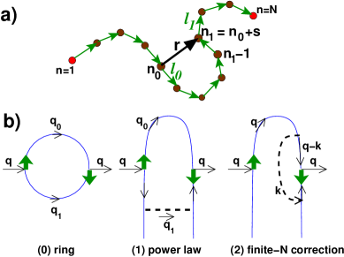
It is generally assumed that large scale correlations are screened in dense solutions of flexible polymers beyond the local correlation length characterizing the decay of the density fluctuations [1, 2, 3]. One consequence of this screening hypothesis is that orientational correlations between two bonds and on the same chain should vanish rapidly for distances and for corresponding curvilinear distances with being the number of monomers spanning the correlation length. See Figure 1 for a sketch of the notations used in this paper with denoting the monomer index, the number of monomers per chain, the root-mean-square end-to-end distance, the monomer number density, the root-mean-square bond length, the effective bond length and the dimensionless chain stiffness parameter [2, 4].
Surprisingly, recent numerical studies [5, 6, 7, 8, 9] have demonstrated the power-law decay of the intrachain bond-bond correlation function , averaged over bond pairs of same curvilinear distance , as a function of
| (1) |
with an exponent rather than the exponential cut-off expected from Flory’s ideality hypothesis [10]. (The amplitude is given in eq 3 below.) This result has been rationalized by means of scaling arguments and perturbation calculations which demonstrate the systematic swelling of the chain segments [11, 5, 12, 13, 7]. The gist of the calculation is that the effective interactions between the monomers of a chain are only partially screened and represented (to leading order) by an effective potential in momentum space
| (2) |
increasing quadratically with wavevector [2, 13]. The detailed calculation yields the power-law amplitude
| (3) |
which is very close to the empirical values for all simulation models tested [7].
Aim and key results of this study.
Since the power-law decay of resembles the return probability of a random walk in three dimensions it is tempting [14] to attribute the observed effect to “self-kicks” of the chain involving the correlated bonds themselves (or their immediate neighbors). Accordingly, the bond-bond correlation function should reveal a -correlation if sampled as a function of the distance between bond pairs. This interpretation turns out to be incorrect, however, and we will show that the power law in simply translates as
| (4) |
with a Flory exponent for (to leading order) Gaussian chains. More specifically, it will be demonstrated by means of analytical theory and Monte Carlo simulation that
| (5) |
as suggested by eq 4, i.e. the angular correlations are genuinely long-ranged. The index “” emphasizes that is the predicted asymptotic behavior for long chains on scales where the system behaves as an incompressible solution. For systems with finite compressibility () the power law generalizes naturally to
| (6) |
in terms of the reduced distance and a scaling function for . Interestingly, the upper cut-off of eq 5 is found to increase rather slowly with chain length
| (7) |
The simulation of computationally challenging chain lengths thus is required to demonstrate numerically the predicted power-law decay of .
Outline.
The one-loop perturbation calculation leading to the above results follows again the seminal work by Edwards [2]. See Figure 1(b) for a sketch of the computed interaction graphs. This calculation will be discussed first (Section 2). Computational methods and parameters are summarized in section 3. We present then in section 4 our numerical results obtained for systems containing either monodisperse polymers or Flory size-distributed equilibrium polymers [15, 16]. By varying the density we scan the screening length over two orders of magnitude [9]. This puts us into a position to test the general scaling relation, eq 6, for systems with finite compressibility. Focusing first on the properties of asymptotically long chains we consider finally the strong finite chain-size effects predicted by eq 7. A synopsis of our results is given in section 5 where we suggest possible avenues for future studies.
2 Perturbation calculation
General remarks.
We remind [2] that the first-order perturbation calculation of a quantity under a perturbation (to be specified below) generally reads . Averages performed over an unperturbed reference system of Gaussian chains of effective bond length are denoted . In this study we have to average the observable over all intrachain bond pairs at a given distance . For linear chains by construction. Thus we only have to compute the average
| (8) |
which simplifies considerably the task compared to the perturbation calculation of the mean-square segment size presented in refs 5, 13, 7. We remind that for closed cycles the ring closure implies long range angular correlations even for Gaussian chains, hence,
| (9) |
to leading order.
We suppose first that the chains are infinite and on local scale perfectly flexible () [17]. We begin by formulating the problem in reciprocal space and demonstrate then the power-law asymptote, eq 5. Finite chain-size effects are first discussed for Flory distributed chains and then by means of inverse Laplace transformation for monodisperse melts. Finally, it is shown how our results can be reformulated for semiflexible chains ().
Reciprocal space description of flexible chains.
The calculation of eq 8 and 9 is most readily performed in reciprocal space as sketched in Figure 1(b). The Fourier transform of a function is denoted , the Laplace transform of a function is written with being the Laplace variable conjugated to the arc-length .
Bond vectors and observable. The vertical bold arrows in Figure 1(b) represent the Fourier transformed bond vectors
| (10) |
with and being the Gaussian distribution function of the bond vector in real and reciprocal space, respectively. We have used here that can be expanded at low momentum [18]. The wavevectors conjugated to the bonds and are denoted and , respectively. The Fourier transform of the observable reads, hence,
| (11) |
Effective potential . The perturbation potential in real space is supposed to be the pairwise sum of the effective monomer interactions of all pairs of monomers of the same chain. To obtain one labels a few chains. The interaction between labeled monomers is (partially) screened by the background of unlabeled monomers. It has been shown [2, 13] that within linear response this corresponds to an effective potential with
| (12) |
This potential is represented by the dashed lines in the diagrams. The bare excluded volume indicated in the first term of eq 12 characterizes the short-range repulsion between monomers. Thermodynamic consistency requires [19, 13, 9] that is proportional to the inverse of the measured compressibility of the solution
| (13) |
where we have introduced a convenient monomeric length and defined the screening length following, e.g., eq 5.38 of ref 2. Please note that can be determined experimentally or in a computer simulation from the low-wavevector limit of the total monomer structure factor and, due to this operational definition, is called “dimensionless compressibility” [9]. The single chain form factor represents the interaction between two monomers caused by the chain connectivity [2]. For Gaussian chains of finite length the form factor is given by Debye’s function [2]. For infinite chains we have, hence, . For scales larger than the screening length () the finite compressibility (indicated by the first term in eq 12) becomes negligible and the solution behaves for all densities as an incompressible melt. Equation 12 reduces thus to the scale-free interaction potential already mentioned (eq 2).
Fourier-Laplace transform of the propagator. We remind that the Fourier transform of the Gaussian propagator[2] may be written with denoting the curvilinear distance between two monomers of the chain. An arrow along a chain contour (thin lines) corresponds to the Fourier-Laplace transformed Gaussian propagator of wavevector as specified in the diagrams. We need to average over all bond pairs at a given distance irrespective of their curvilinear distance and we have thus to sum below over all possible . For infinite chains this corresponds to setting for the corresponding Laplace variable and we shall often use the summed up Gaussian propagator , i.e. the Fourier transform of the density around a reference monomer of all monomers belonging to the same infinite Gaussian chain [3]. Hence,
| (14) |
for infinite chains on large scales ().
Interaction diagrams. The momentum inserted in the interaction diagrams is conjugated to the distance between both bonds. Momentum is a conserved quantity flowing from one correlated point to the other. If the momentum flows in the opposite direction of a bond (as it is the case for the second bond ) the wavevector comes with a negative sign in eq 11. The first two diagrams are thus given by the convolution integrals
| (15) | |||||
| (16) | |||||
The integrals and describe the bond-bond correlation functions of closed cycles and linear chains, respectively. The perturbation calculation of linear chains using eq 8 implies a minus sign. This sign is indicated in front of the effective interaction in the last equation. Using eq 11 and assuming eq 14 the integrals are considerably simplified
| (17) | |||||
| (18) |
and the inverse Fourier transforms are thus
| (19) | |||||
| (20) |
Sum rule for closed cycles and linear chains.
Up to a constant prefactor the integrals and are thus equal on large scales (). This remarkable result needs further discussion beyond the technical notions set up in the preceding paragraph.
Closed cycles. The bond-bond correlation function of closed rings is directly obtained from after normalization with the density
| (21) |
The reason for the normalization factor is that for both bonds are known to be bonds of the same polymer ring while the interaction integral eq 15 corresponds only to a probability for both bonds being in the same chain times a probability that this chain is closed. That is negative is of course due to the closure constraint which corresponds to an entropic spring force bending the second bond back to the origin. Since this force is scale free (for infinite chains) this yields a power law.
Linear chains. It follows immediately from eq 20 that for linear chains
| (22) |
which demonstrates finally the key claim (eq 5) made in the Introduction (assuming ). The normalization factor is due to the fact that for both bonds are known to belong to the same chain. As compared to the closed cycles the correlation has the opposite sign since the attractive spring of the ring closure (indicated by in eq 17) has been replaced by the effective repulsion (indicated by in eq 18). This repulsion bends the second bond away from the origin increasing thus the bond-bond correlation function.
Sum rule. Interestingly, the perturbation result, eq 19, may be rewritten as
| (23) |
where we have used the normalization factors mentioned above. This “sum rule” suggests a geometrical interpretation of the observed relation between infinite linear chains and closed cycles which may remain valid beyond the one-loop approximation used here. The idea is that in an hypothetical ideal melt containing both linear chains and closed cycles all correlations disappear (on distances much smaller than the typical chain sizes) when summed up over the contributions of both architectures. The weight corresponds to the fraction of bond pairs in closed loops [20]. Since the orientational correlations in ideal cycles are necessarily long-ranged due the ring closure (eq 21), it follows, assuming the sum rule, that the same applies to bond pairs of linear chains. Since bonds in closed cycles are anti-correlated (), they must be aligned () for linear chains.
Flory size-distributed chains.
We turn now to the upper boundary indicated in eq 5 and attempt to characterize finite- effects for . We start by considering self-assembled chains (branching of chains and formation of closed loops being disallowed) having an annealed size-distribution [16] with an exponentially decaying number density for polymer chains of length with being the chemical potential. This so-called “Flory size-distribution” is relevant to equilibrium polymer systems [15, 6]. For Flory distributed Gaussian chains the form factor becomes [13] in the intermediate wavevector regime. Since the first term in eq 12 can again be neglected in the incompressible limit (), this yields an effective excluded volume
| (24) |
i.e. the term in eq 2 is replaced by . Since this applies also for the propagator, which becomes , the central eq 14 remains valid for Flory distributed chains and, hence, also the sum rule eq 23. We compute as before eq 20 using now the inverse Fourier transform of in real space
| (25) |
This yields with denoting the asymptotic power law eq 5 (with ) and
a rapidly decaying function of with being the typical end-to-end distance of the polydisperse system.
Interestingly, the diagram (1) is not sufficient to characterize the bond-bond correlation for larger distances since the last diagram (2) of Figure 1(b) corresponding to the convolution integral
| (26) | |||||
provides, as we shall see, the actual cut-off of the power law in this limit. Using again eq 11 and eq 14 the integral factorizes
| (27) | |||||
| (28) |
where we have introduced in the last line the convenient dimensionless constant
| (29) |
in which we dump local physics at large wavevector . Before evaluating the angular correlations in real space it is important to clarify the physics described by the diagram. The underlined second factor in eq 27 characterizes the alignment of the bond vectors of the monomers and at a fixed distance of the monomers and (Figure 1(a)). Obviously, even for Gaussian chains these two bonds become more and more aligned if the distance gets larger than , i.e. when the chain segment becomes stretched. For perfectly Gaussian chains the bonds and at and would still remain uncorrelated, however, since the second bond is outside the chain segment on which we have imposed the distance constraint.
As indicated by the dashed line in the diagram, it is then due to the effective interaction between the monomers within the stretched segment () and the monomers outside () that the bonds at and get aligned and then in turn the two bonds at and . We note that, strictly speaking, depends on the mean chain length , since is a function of . However, one checks readily that this effect can be neglected for reasonable mean chain lengths. We also note that the constant is finite, since the UV divergence which formally arises for large (where ) may be regularized by local and, hence, model dependent physics [21]. We will determine numerically from our simulations of self-assembled linear equilibrium polymers (Section 4).
Assuming a finite and chain length independent coefficient in eq 28 and inserting the propagator for Flory distributed chains we obtain by inverse Fourier transformation
| (30) |
for the interaction integral in real space. Normalizing as before with and summing over both diagrams this yields
| (31) |
for . Comparing both terms in eq 31 one verifies that the crossover occurs at in agreement with eq 7. The bond-bond correlation function of an incompressible solution of Flory distributed polymers becomes thus constant for . This remarkable result is essentially due to the polydispersity. This allows to find for all distances pairs of bonds and stemming from segments which are slightly stretched by an energy of order and which are, hence, slightly shorter than a unstretched segment of length . Since there are more shorter chains and chain segments this just compensates the decay of the weight due to the weak stretching. Although the number of such slightly stretched segments decays strongly with distance, their relative effect with respect to the typical unstretched segments, , remains constant for all . It is for this reason that the chemical potential appears in the second term of eq 31. Please note that bond pairs from strongly stretched segments (corresponding to an energy much larger than ) are, however, still exponentially suppressed and can be neglected. As we will show now, this is different for monodisperse chains where strongly stretched chain segments contribute increasingly to the average for large distances.
Finite chain size effects: Monodisperse chains.
The bond-bond correlation function of monodisperse polymer melts may be obtained by inverse Laplace transformation of the result obtained for Flory distributed grand-canonical polymers. Note that a very similar calculation has been described in detail in ref 13 for the coherent structure factor. The interaction integral for monodisperse chains of chain length in reciprocal space may we written
| (32) |
where denotes the Laplace transform of a function . The extra factor stands for the dangling tails in both diagrams which accounts for the combinatorics necessary due to the finite chain length. and are the interaction integrals computed in the previous paragraph using eq 24 for the effective interaction potential and the corresponding Fourier-Laplace transformed propagator . Note that the first term in eq 32 is accurate up to finite-size corrections due to the use of eq 24 for the effective potential.
We compute then the inverse Fourier transformation and normalize it consistently with using eq 25. This yields
| (33) |
with and defined as for Flory distributed chains (eq 29). The first term due to diagram (1) of Figure 1(b) contains a (rapidly decaying) cut-off function
with denoting the repeated integral of the complementary error function [22]. This function is non-monotic and goes through a maximum with an overshoot of about at . The second term in eq 33 is again due to diagram (2). The function
becomes constant for small where . We note that as for Flory distributed chains the second term in eq 33 becomes dominant on scales . Interestingly, for large we have and is, hence, predicted to increase as
| (34) |
We remind that for a chain segment of arc-length stretched between its end monomers and one expects if . The coefficient stands for the correlation of the bond at monomer within the stretched segment with the bond at the monomer outside the segment (Figure 1(b)). The limiting behavior, eq 34, is thus expected since more and more bond pairs from strongly stretched chain segments with must contribute to the average at distances .
Finite persistence length effects.
Up to now we have supposed that the chains are perfectly flexible. For semiflexible chains () the above results apply now to the Kuhn segments of the chains [23]. The bond length of the Gaussian reference chain used in the perturbation calculation corresponds to the length of the Kuhn segment (i.e. not to the effective bond length ), the arc-length to the number of Kuhn segments and the density to the density of Kuhn segments
| (35) |
If the bond-bond correlation function calculated in terms of Kuhn segment units is reexpressed in the natural microscopic units, eq 35 introduces the additional prefactor indicated in eq (5).
3 Algorithmic and technical issues
The theoretical predictions derived above are supposed to hold in any dense polymer solution containing sufficiently long chains. The numerical data presented below (Figures 2-4) have been obtained using the well-known “bond fluctuation model” (BFM) [24, 25, 26, 7, 8, 9, 15] — an efficient lattice Monte Carlo scheme where a coarse-grained monomer occupies 8 lattice sites on a simple cubic lattice (i.e., the volume fraction is ) and bonds between adjacent monomers can vary in length and direction [27]. All length scales are given in units of the lattice constant and we set . Even the partial overlap of monomers is forbidden in the classical formulation of the BFM [24, 25, 7, 15]. We have put the predictions to a test by simulating systems having either a quenched and monodisperse or an annealed size distribution:
(i) Monodisperse systems have been equilibrated and sampled using a mix of local, slithering snake, and double bridging Monte Carlo moves. See ref 7 for details. Systems with chain lengths up to have been obtained for various densities, as indicated in Figure 2, up to the “melt density” [7]. We use periodic simulation boxes of linear size . For the largest density used this corresponds to monomers and to chains of length per simulation box. The smallest density indicated () refers to one single chain in the box allowing us to characterize properly the dilute reference point. The scaling of bond-bond correlation function with chain length at is presented in Figure 3.
(ii) As sketched in Figure 4, systems with annealed size distribution — so-called “equilibrium polymers” — have been obtained by attributing a finite and constant scission energy to each bond which has to be paid whenever the bond between two monomers is broken. Standard Metropolis Monte Carlo is used to reversibly break and recombine the chains [15, 13, 6]. Branching and formation of closed rings are explicitly forbidden. As one expects from standard linear aggregation theory, the density of chains shows essentially a Flory distribution, , with the mean chain size scaling as [15]. Only local hopping moves have been used for sampling equilibrium polymer systems, since the breaking and recombination of chains reduce the relaxation times dramatically compared to monodisperse systems [28].
4 Simulation results
Density effects.
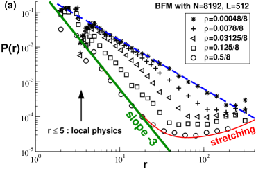
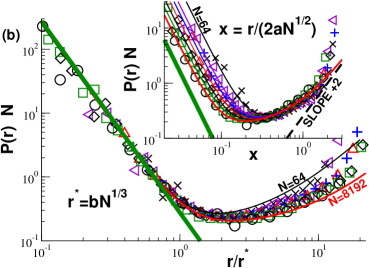
The scaling of the bond-bond correlation function with density for monodisperse chains is addressed in Figure 2. Only data for our largest chain length is presented here to focus first on the discussion of the large- limit. The finite- effects, visible nevertheless (“stretching”) from the increase of for large , will be further discussed below at the end of this section (Figures 3 and 4). As can be seen in panel (a), model-depending physics not taken into account by the theory obviously becomes relevant for short distances corresponding to segments of a couple of monomers. For clarity we have thus omitted data points with in all other figures and panels below.
The power-law behavior observed for small densities is implicit to the swollen-chain statistics in dilute good solvents where the root-mean-square segment size is known to scale with a Flory exponent (with denoting the respective power-law amplitude). Since with (see ref 5) it follows from eq 4 that the bond-bond correlation function should scale as
| (36) |
as indicated by the dashed lines in Figure 2. The index indicates that this is the expected asymptotic behavior for asymptotically long chains in the dilute good solvent limit.
As the density increases, the correlation function still coincides with the dilute behavior for distances smaller than the screening length of the semidilute solution where each chain segment interacts primarily with itself. (The screening length is indicated in the inset of panel (b).) At distances , where the chains overlap and form a “melt of blobs”, [3] the correlation function decreases much faster, however not exponentially as one might expect from Flory’s hypothesis or the -scenario (“self-kicks”) mentioned in the Introduction, but with a second power-law regime with exponent .
That the crossover between both power-law regimes occurs indeed at can better be seen from panel (b) where we have replotted the data as a function of the reduced distance as suggested by eq 6. Taking apart the finite chain-size effects for large distances we find an excellent scaling collapse of the data considering the large spread of the raw data (panel (a)) and that no free shift parameter was used. The three independently determined length scales , and used for the rescaling according to eq 6 are compared in the inset of panel (b). The latter two lengths are relevant due to the stiffness parameter which is needed (eq 5) for the vertical scale . Note that the bond length (triangles) is essentially constant for all densities, at least on the logarithmic scales addressed here. The effective bond length approaches from above, i.e. decreases with increasing . The dashed line in the inset corresponds to the power law expected from the scaling theory of semidilute solutions [3]
| (37) |
Thus, the density dependence of can not be neglected. The screening length has been determined assuming eq 13 and using the directly measured effective bond length and dimensionless compressibility . We have crosschecked these values with the decay of the total structure factor where this has been possible. For not too high densities our data is nicely fitted by the power law (bold line)
| (38) |
as expected for semidilute solutions.[3] Obviously, the semidilute power-law relations cannot hold strictly for the highest densities where the compressibility (and, hence, the blobs size) becomes too small [26, 29]. However, the differences are small on logarithmic scales and we obtain a very similar scaling plot by insisting on eqs 37 and 38 for all densities (not shown).
The density crossover scaling implies obviously the matching of the dilute and dense asymptotic power-law predictions
| (39) |
As can be checked using the well-known scaling relations , and defining the semidilute solution [3] (which are also implicit to eq 37 and eq 38), eq 39 requires the prefactor in eq 5. We have checked that scales the data, while without does not (not shown). The successful scaling collapse confirms, hence, the rescaling of the Kuhn segments presented at the end of section 2.
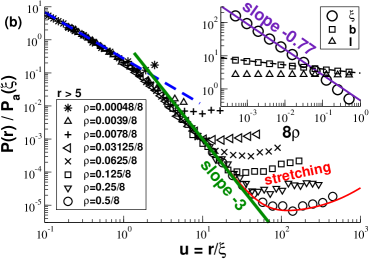
Finite -effects for monodisperse chains.
We concentrate in the reminder of this section on dense melts with . Chain length effects are investigated in Figure 3 for monodisperse chains. The unscaled raw data are presented in panel (a). As expected from theory, increases for large distances due to the increasing weight of stretched segments contributing to the average at distance . With increasing chain length this effect becomes less important, however, and our data approaches systematically the asymptotic power-law decay (eq 5) indicated by the bold line. The thin lines represent the complete prediction, eq 33, for different . Numerical data and theory agree nicely, especially for large chains. The deviations observed for and for fully stretched chains () are, of course, expected. Please note that the cut-off function of the asymptotic power law obtained by diagram (1) may be ignored () without changing the plot. The finite- effects are in fact dominated by the function of the second term in eq 33. We remind that eq 34 predicts ultimately a quadratic increase with distance of the bond-bond correlation function as indicated by the dashed line for one chain length (). It is essentially the limited simulation box size () of the present study preventing us from demonstrating numerically this asymptotic behavior which should be accessible otherwise for the longer chains ().
The scaling with chain length is addressed in panel (b). Obviously, eq 33 is not compatible with one scaling variable allowing to collapse all data. The crossover from the power-law asymptote (diagram (1)) to the -dependent correction (due to diagram (2)) is, however, well described by plotting as a function of with using as a scale the minimum of eq 33. As shown in the main panel this yields a numerically satisfactory scaling over two orders in magnitude of the reduced distance , especially for our largest chains. This scaling fails for large distances (), however, as emphasized by the theoretical predictions (thin lines) indicated for and (bottom). In this limit only the second term in eq 33 matters and, as can be seen from the inset in Figure 3(b), a data collapse can be achieved by tracing as a function of . As already noted, the observed deviations from the limiting behavior for (eq 34) are expected (i) due to the breakdown of the Gaussian chain model at for small chain lengths and (ii) due to the restricted box size of the present study.
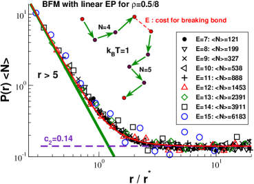
Equilibrium polymers.
Fortunately, this scaling issue is much simpler for equilibrium polymers as shown in Figure 4 where we have plotted as a function of with using the indicated mean chain lengths . Note that the error bars (not shown) become clearly much larger than the symbol size for large bond energies . It is fair to state, however, that all data points collapse nicely on the one master curve indicated by the thin line obtained from eq 31 for . That the variable effectively drops out stems from (i) the rapid decay of the exponential cut-off function of the first term in eq 31 and (ii) the -independence of the correction term. That the bond-bond correlation function of equilibrium polymers becomes constant for large distances confirms a non-trivial prediction of the theory. We used the clearly visible plateau to determine the coefficient required for the interaction diagram (2) and already used in the previous Figures 2 and 3. We note finally that this best fit value of is rather close to , the independently determined bond-bond correlation between adjacent bond vectors [21].
5 Conclusion
Summary.
Focusing on dense solutions of linear and (essentially) flexible polymer chains we have investigated analytically and by means of Monte Carlo simulation the intrachain angular correlations with respect to the distance between bond pairs. Motivated by recent work showing the power-lay decay of the bond-bond correlation function with curvilinear distance (eq 1) we addressed the question whether the correlations are indeed long-ranged in space or only due to the return probability (“self-kicks”) of a chain. Our calculations of have been based on a standard one-loop perturbation scheme (Figure 1(b)). The power-law decay predicted for asymptotically long chains (eq 5) is well confirmed by our numerically data approaching systematically the asymptotic envelope with increasing density (Figure 2) and (mean) chain length (Figures 3 and 4). As postulated in eq 6, density effects are found to scale as with being the independently measured screening length. For we confirm the expected power law for dilute good solvents (eq 36). More importantly, the explicit compressibility dependence of the bond-bond correlation function drops out for where , i.e. polymer solutions behave on large scales as incompressible packings of blobs and this for all densities provides that the chains are sufficiently long. Finite-chain size effects are also successfully predicted by the theory for both monodisperse polymers (eq 33) and equilibrium polymers (eq 31). It should be emphasized that the fit to the asymptotic power law is parameter free and that fitting the -effect only requires one additional free parameter, (eq 28), due to local orientational correlations between adjacent bonds which regularize diagram in Figure 1(b).
Outlook.
Interestingly, the presented perturbation calculation for dense polymer chains may also be of relevance to the angular correlations of dilute polymer chains at and around the -point which has received attention recently [14]. The reason for this connection is that (taken apart different prefactors) the same effective interaction potential (eq 2) enters the perturbation calculation in the low wavevector limit. We expect therefore similar genuinely long-ranged angular correlations for asymptotically long -chains (as implied by eq 4) rather than the “self-kicks” suggested in the literature [14]. Strong finite- effects are again expected, however, and much longer chains as the ones presented in the current numerical studies of -chains are required to demonstrate the asymptotic power-law behavior.
The present study has focused on the first Legendre polynomial of the intrachain bond-bond correlations [10]. Since this is not an easily experimentally accessible property it should be mentioned that higher Legendre polynomials have also been predicted following similar perturbation calculations as the ones presented above. For instance it is possible to show that the second Legendre polynomial should decay as the fifth power of distance if averaged over all intra-chain contributions and as the sixth power if averaged over all bond pairs at a given distance [30]. Unfortunately, we are at present unable to demonstrate these predictions numerically due to the stronger power-law decay requiring much better statistics. This study is currently underway.
Our one-loop perturbation calculation show that for infinite chains or Flory distributed (grand-canonical) polymers the bond-bond correlations observed in systems of linear chains are equivalent to the subtraction of angular correlations due to closed cycles (eq 23). The same sum rule can be shown to hold for higher Legendre polynomials summing over intra- and inter-chain contributions. This finding suggests a deeper purely geometrical description of the observed long-ranged orientational correlations relating this issue to the recently discovered Anti-Casimir forces in polymer melts [19, 31] arising due to a similar subtraction of soft fluctuation modes, not present in the linear polymer system but in its hypothetical counterpart containing both chain architectures. Taking advantage of the polymer-magnetic analogy[3] we plan to address this fundamental connection in a more theoretical paper.
Acknowledgment. We thank A.N. Semenov (ICS, Strasbourg, France) for helpful discussions. Financial support by the University of Strasbourg, the CNRS, the IUF and the ESF-STIPOMAT programme are acknowledged as well as a generous grant of computer time by the IDRIS (Orsay).
References
- [1] Flory, P. J. J. Chem. Phys. 1949, 17, 303.
- [2] Doi, M.; Edwards, S. F., The Theory of Polymer Dynamics (Clarendon Press, Oxford, 1986).
- [3] de Gennes, P. G., Scaling Concepts in Polymer Physics (Cornell University Press, Ithaca, New York, 1979).
- [4] The local properties , , or are supposed to be those of asymptotically long chains. The determination of their values requires the numerically extrapolation using the data obtained from a systematic chain length variation. Extrapolation schemes for the dimensionless compressibility and the effective bond length are, e.g., discussed in ref 9.
- [5] Wittmer, J. P.; Meyer, H.; Baschnagel, J.; Johner, A.; Obukhov, S. P.; Mattioni, L.; Müller, M.; Semenov, A. N. Phys. Rev. Lett. 2004, 93, 147801.
- [6] Wittmer, J. P.; Beckrich, P.; Crevel, F.; Huang, C. C.; Cavallo, A.; Kreer, T.; Meyer, H. Comp. Phys. Comm. 2007, 177, 146.
- [7] Wittmer, J. P.; Beckrich, P.; Meyer, H.; Cavallo, A.; Johner, A.; Baschnagel, J. Phys. Rev. E 2007, 76, 011803.
- [8] Meyer, H.; Wittmer, J. P.; Kreer, T.; Beckrich, P.; Johner, A.; Farago, J.; Baschnagel, J. Eur. Phys. E 2008, 26, 25.
- [9] Wittmer, J. P.; Cavallo, A.; Kreer, T.; Baschnagel, J.; Johner, A. J. Chem. Phys. 2009, 131, 064901.
- [10] Differences between our definition of the bond-bond correlation function and the more common first Legendre polynomial using the normalized tangent vector can be shown to be negligible.
- [11] Semenov, A. N.; Johner, A. Eur. Phys. J. E 2003, 12, 469.
- [12] Wittmer, J. P.; Beckrich, P.; Johner, A.; Semenov, A. N.; Obukhov, S. P.; Meyer, H.; Baschnagel, J. Europhys. Lett. 2007, 77, 56003.
- [13] Beckrich, P.; Johner, A.; Semenov, A. N.; Obukhov, S. P.; Benoît, H. C.; Wittmer, J. P. Macromolecules 2007, 40, 3805.
- [14] Shirvanyants, D.; Panyukov, S.; Liao, Q.; Rubinstein, M. Macromolecules 2008, 1, 1475.
- [15] Wittmer, J. P.; Milchev, A.; Cates, M. E. J. Chem. Phys. 1998, 109, 834.
- [16] Concerning static equilibrium properties there is no difference between an annealed and a corresponding quenched polydispersity for infinite macroscopically homogeneous systems. This follows from the well-known behavior of fluctuations of extensive parameters in macroscopic systems: the relative fluctuations vanish as as the total volume . The latter limit is taken first in our calculations, i.e. we consider an infinite number of (annealed or quenched) chains. The large chain limit is then taken afterwards to increase the range of the scale free limit (eq 5).
- [17] The two lengths and (or ) are nevertheless given if this is helpful to remind well-known relations and to indicate where the different contributions stem from.
- [18] Equation 10 does not only apply to Gaussian bonds, but to the low-wavevector limit of any bond vector with an analytic bond length distribution [7].
- [19] Semenov, A. N.; Obukhov, S. P. J. Phys.: Condens. Matter 2005, 17, 1747.
- [20] We remember that is the density of all the monomers of an infinite chain with the reference monomer being at the origin. Hence, sums over the monomers of both strands connected to the reference monomer. We know for linear chains as for cycles that both bonds are connected by a first strand. The probability for both bonds to be in a closed loop is given by the density of the second strand. The factor is thus needed to avoid counting the same cycle twice.
-
[21]
For soft melts with weak bare excluded volume , i.e. , it can be
shown that an upper cut-off wavevector regularizes the
integral over . The coefficient becomes
Using and for this gives . This is not that far off the best fit value considering that for small one expects to be rather determined by the model-depending stiffness between adjacent bonds.(40) - [22] Abramowitz, M.; Stegun, I. A., Handbook of Mathematical Functions (Dover, New York, 1964).
- [23] Rubinstein, M.; Colby, R., Polymer Physics (Oxford University Press, Oxford, 2003).
- [24] Carmesin, I.; Kremer, K. Macromolecules 1988, 21, 2819.
- [25] Deutsch, H.; Binder, K. J. Chem. Phys. 1991, 94, 2294.
- [26] Paul, W.; Binder, K.; Heermann, D.; Kremer, K. J. Phys. II 1991, 1, 37.
- [27] We have crosschecked our lattice Monte-Carlo results by molecular dynamics simulation of a standard bead-spring model [5, 7, 8]. Sampling dense melts with chain lengths up to we obtain the same qualitative behavior albeit the power-law asymptote is less convincingly shown as one expects due to the much shorter chain length.
- [28] Huang, C. C.; Xu, H.; Crevel, F.; Wittmer, J.; Ryckaert, J.-P., in Computer Simulations in Condensed Matter: from Materials to Chemical Biology (Springer, Lect. Notes Phys., International School of Solid State Physics, Berlin/Heidelberg, 2006), Vol. 704, pp. 379–418.
- [29] Foteinopoulou, K.; Karayiannis, N. C.; Laso, M.; Kröger, M.; Mansfield, M.-L. Phys. Rev. Lett. 2008, 101, 265702.
-
[30]
Concerning the general Legendre polynomial characterizing the angular
correlations of bond pairs summing over both intra- and inter-chain
contributions we find analytically
with being the degree of the Legendre polynomial and the spatial dimension. The simulation of polymer melts in thin films () may thus allow to demonstrate more readily the suggested behavior for higher () Legendre polynomials. - [31] Obukhov, S. P.; Semenov, A. N. Phys. Rev. Lett. 2005, 95, 038305.
Title: Distance dependence of angular correlations in dense polymer solutions
Authors: J.P. Wittmer, A. Johner, S.P. Obukhov, H. Meyer, A. Cavallo, J. Baschnagel
![[Uncaptioned image]](/html/0912.3340/assets/x7.png)
For Table of Contents (TOC) use only.