Abelian Sandpile Model on the Honeycomb Lattice

Abstract

We check the universality properties of the two-dimensional Abelian sandpile model by computing some of its properties on the honeycomb lattice. Exact expressions for unit height correlation functions in presence of boundaries and for different boundary conditions are derived. Also, we study the statistics of the boundaries of avalanche waves by using the theory of SLE and suggest that these curves are conformally invariant and described by SLE₂.
PACS: 05.65+b, 89.75.Da

1 Introduction

Bak, Tang and Wiesenfeld introduced the theory of self-organized criticality as a general mechanism that can explain the behaviour of complex systems which naturally organize themselves into a critical state [1]. They defined the sandpile model as an example of slowly driven and dissipative complex system to explain the concept of self-organized criticality. Thanks to the Abelian property of the model [2], many statistical and dynamical results have been derived exactly. Among the main analytical results obtained for the isotropic two-dimensional model, one can mention 1-site probabilities of height variables [3], bulk correlations of height 1 variables and of some specific clusters known as weakly allowed clusters [4, 5, 6], the discussion of boundary conditions [7, 8] and the effect of boundaries on height probabilities [9, 10, 11, 12, 13], boundary correlations of height variables [14, 15, 16], bulk correlations of higher height variables [17] and avalanche and toppling wave distributions [18, 19, 20, 21]. The sandpile model has been investigated in the continuum limit and from a field theoretical perspective. It has been shown that the Abelian sandpile model can be described by a specific logarithmic conformal field theory, with central charge $c=-2$ [5, 22, 13, 17].

Most of the results, analytical or numerical, have been obtained when the sandpile model is formulated on the square lattice. In fact, the simple and symmetric structure of the square lattice make it easier to carry out some of the lattice calculations. However, other regular two-dimensional lattices have been considered. Height probabilities and critical exponents of the sandpile model on the triangular and honeycomb lattices have been investigated using renormalization group transformations and numerical simulations [23, 24]. Moreover the critical exponents and the finite-size scaling functions for the avalanche wave distributions on the square, honeycomb, triangular, and random lattices have been evaluated from Monte Carlo simulations [25]. The results clearly suggest that the model on different lattices has the same set of critical exponents and scaling behaviour.

In this paper, we study the Abelian sandpile model on the honeycomb lattice. The structure of the honeycomb lattice is more complicated than the square lattice, as there are two lattice points in each unit cell. However, the correspondence between recurrent configurations and spanning trees is maintained, and an exact expression for the Green function can be obtained, along with the exact asymptotic value. These are the two main ingredients to perform the lattice calculations and in turn, to check explicitly the universal behaviour of the model. We do that by looking at the universal terms of the unit height correlation functions with and without boundaries.

The universality in the critical behaviour of sandpile model can be also checked from the point of view of geometrical features of the model. Indeed the dynamics of the model is such that each avalanche is formed on a compact domain with a boundary which converges to a fractal curve in the scaling limit [26]. For the sandpile model defined on the square lattice, it has been recently suggested that the boundary of these avalanche clusters belongs to the family of conformally invariant curves generated by the Schramm-Loewner evolution process SLE_κ, for a diffusitivity constant $\kappa=2$ [27].

Avalanches can be also decomposed into a sequence of simpler objects called toppling waves. While avalanches are believed to be described by a multifractal set of scaling exponents and have a complex scaling behaviour, waves show simple scaling properties and are more convenient for the analysis of avalanche statistics. Here, we also check the universality properties by studying the statistics of toppling wave boundaries for the model defined on the honeycomb lattice.

This paper is organized as follows: in the next section we define the sandpile model on the honeycomb lattice and give the exact (and well-known) expression for the discrete Green function on the lattice. In the third section, we review the methods used for our lattice calculations and then give the details of the results in Section $4$. We compare our results with the predictions of the $c=-2$ conformal field theory in Section $5$. Finally, we investigate in Section 6 the statistics of the toppling wave boundaries on the honeycomb lattice and verify its universality. We finish with some conclusions. The values of the lattice Green function for small distances are listed in an Appendix, which also contains the details for the calculations of its asymptotic behaviour for large distances.

2 The sandpile model

We start by defining the sandpile model on a two-dimensional honeycomb lattice of linear size $L$ and with $N$ sites. To each site of the lattice a random integer variable $h\in\{1,2,3\}$ is assigned which can be interpreted as the number of sand grains at that site. A configuration is characterized by the set of heights of all sites and is called stable if the height values are equal to 1, 2 or 3.

The dynamics of the model is defined in two steps: $1)$ given a stable configuration, a grain of sand is added to a randomly chosen site, so that its height is increased by one, while the other sites remain unchanged; $2)$ if the height of that site becomes greater than the critical height $h_{c}=3$, the site becomes unstable, topples and loses three grains of sand, each one of which drops on one of the nearest neighbours. The toppling rule can be written in the form $h_{j}\to h_{j}-\Delta_{ij}$ for all sites $j$, where $\Delta_{ij}$ is called the toppling matrix and is equal to the discrete Laplacian, namely

$$\Delta_{ij}=\cases{3&if $i=j$,\cr-1&if $i$ and $j$ are nearest neighbours,\cr 0&otherwise.}$$ (2.1)

If, as a result of this toppling, some of the neighbours become unstable, the toppling process continues until all sites become stable and the avalanche ends. Thus in each time step, the dynamics takes the system from a stable configuration to another stable configuration.

For a lattice with $N$ sites, the total number of stable configurations is $3^{N}$, but not all of them occur in the steady state. The stable configurations are divided into two classes: recurrent and transient. After a long time, when the system enters the steady state, the transient configurations have zero probability of occurrence and all recurrent configurations occur with equal probability [2]. The burning algorithm allows to determine whether a given configuration is recurrent or not, and also establishes a one-to-one correspondence between recurrent states and spanning trees. Thus one can compute the total number of recurrent configurations by enumerating the spanning trees. From Kirchhoff’s theorem, the number of spanning trees is given by the determinant of the toppling matrix $\Delta$, or the discrete Laplacian matrix.

If we keep the form of the toppling matrix as above in (2.1), even for the boundary sites which have strictly less than three neighbours, then sand grains will leave the system each time a boundary site topples. Such sites are therefore dissipative and called open. If we set the diagonal element $\Delta_{ii}$ equal to the number of neighbours of $i$, then $i$ is conservative and called closed. Boundary sites can freely be chosen open or closed; the dynamics of the model, described above, is well-defined provided the system contains at least one open site.

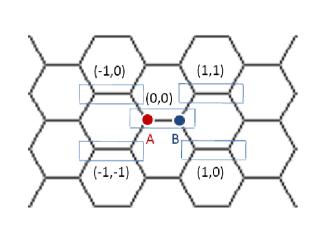
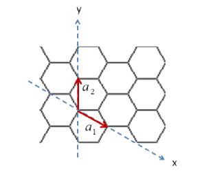
$(a)$	$(b)$

Figure 1: $(a)$ A portion of the honeycomb lattice with the unit cells, marked by rectangles. Each unit cell contains two types of lattice sites, $A$ and $B$. $(b)$ The coordinate system used to label the cells is spanned by the two unit vectors $\vec{a}_{1}$ and $\vec{a}_{2}$.

The honeycomb lattice can be divided into unit cells such that each cell contains two lattice points, one of type $A$ (left site) and one of type $B$ (right site), as shown in Fig.1a. We choose the origin of the coordinate system at a site of type $A$. The position of a cell is specified by the vector $n\vec{a}_{1}+m\vec{a}_{2}$, where $\vec{a}_{1}$ and $\vec{a}_{2}$ are the unit vectors shown in Fig.1b and $n,m$ are integer numbers in ${{Z}}$. Then, each site is characterized by the location of its cell, $\vec{r}=(n,m)$, and its location inside the cell, as $\alpha=0,1$ for $A$-type or $B$-type sites respectively. So the complete coordinates of a lattice site is a triplet $(n,m;\alpha)$. We will also use polar coordinates $(n,m)\leftrightarrow(r,\varphi)$ such that $\vec{r}=re^{i\varphi}$, with $r$ the Euclidean distance to the origin given by $r^{2}=n^{2}+m^{2}-nm$ and $\varphi$ the angle measured counterclockwise from the $\hat{n}$ axis. Explicitly the change of coordinates reads $n=r\cos{\varphi}+{r\over\sqrt{3}}\sin{\varphi}$ and $m={2r\over\sqrt{3}}\sin{\varphi}$ (so $(r,\varphi)$ are the polar coordinates of the site $(n,m;0)$).

The diagonalization of $\Delta$ can be obtained by a method based on the decomposition of the lattice into unit cells [29]. One can write the connectivity between the vertices of the unit cells $\vec{r}_{1}=(n_{1},m_{1})$ and $\vec{r}_{2}=(n_{2},m_{2})$ in terms of $2\times 2$ adjacency matrices $a(\vec{r}_{1};\vec{r}_{2})$ given by

$$a_{\alpha_{1}\alpha_{2}}(\vec{r}_{1};\vec{r}_{2})=\cases{1&if site $\alpha_{1}$ in cell $\vec{r}_{1}$ and site $\alpha_{2}$ in cell $\vec{r}_{2}$ are adjacent,\cr 0&otherwise.}$$ (2.2)

As they only depend on the difference $\vec{r}=\vec{r}_{2}-\vec{r}_{1}$, we will write $a(\vec{r})\equiv a(\vec{r}_{1};\vec{r}_{2})$. Explicitly the connectivity matrices of each unit cell with itself and its four neighboring cells read (rows and columns are labelled by $\alpha_{1},\alpha_{2}=0,1$ in that order)

$$a(0,0)=\pmatrix{0&1\cr 1&0},\qquad a(1,0)=a(1,1)=a^{t}(-1,0)=a^{t}(-1,-1)=\pmatrix{0&0\cr 1&0},$$ (2.3)

while all the other matrices equal to 0. The Laplacian can then be written as

$$\Delta_{(\vec{r}_{1};\alpha_{1}),(\vec{r}_{2};\alpha_{2})} \!\!\!=\!\!\! [3-a(0,0)]\otimes\delta_{\vec{r}_{2},\vec{r}_{1}}-a(1,0)\otimes\delta_{\vec{r}_{2},\vec{r}_{1}+\vec{a}_{1}}-a(-1,0)\otimes\delta_{\vec{r}_{2},\vec{r}_{1}-\vec{a}_{1}}$$ (2.4)

$$\hskip 14.22636pt-\;a(1,1)\otimes\delta_{\vec{r}_{2},\vec{r}_{1}+\vec{a}_{1}+\vec{a}_{2}}-a(-1,-1)\otimes\delta_{\vec{r}_{2},\vec{r}_{1}-\vec{a}_{1}-\vec{a}_{2}}.$$

Let us consider an $N_{1}\times N_{2}$ array of unit cells with periodic boundary conditions, namely the set of cells $\vec{r}=(n,m)$ with $1\leq n\leq N_{1}$, $1\leq m\leq N_{2}$ and periodicity in both coordinates. In the decomposition (2.4), the matrices acting in the $\vec{r}$ space are made of cyclic matrices and are simultaneously diagonalized by going to the basis of eigenfunctions $v_{k_{1},k_{2}}(n,m)=e^{2i\pi k_{1}n/N_{1}}\,e^{2i\pi k_{2}m/N_{2}}$. In this basis, the Laplacian is block-diagonalized, $\Delta\sim\oplus_{\theta_{1},\theta_{2}}\>M(\theta_{1},\theta_{2})$, with

$$M(\theta_{1},\theta_{2}) \!\!\!=\!\!\! 3\,{{I}}-a(0,0)-a(1,0)e^{i\theta_{1}}-a(-1,0)e^{-i\theta_{1}}-a(1,1)e^{i(\theta_{1}+\theta_{2})}-a(-1,-1)e^{-i(\theta_{1}+\theta_{2})}$$ (2.5)

$$\!\!\!=\!\!\! \pmatrix{3&-1-e^{-i\theta_{1}}-e^{-i(\theta_{1}+\theta_{2})}\cr-1-e^{i\theta_{1}}-e^{i(\theta_{1}+\theta_{2})}&3},$$

where the angles are given by $\theta_{j}={2\pi k_{j}\over N_{j}}$, with $0\leq k_{1}\leq N_{1}-1$ and $0\leq k_{2}\leq N_{2}-1$.

From the previous results, we readily obtain

$$\det\Delta=\prod_{\theta_{1},\theta_{2}}\det M(\theta_{1},\theta_{2})=\prod_{\theta_{1},\theta_{2}}\Big{[}6-2\cos\theta_{1}-2\cos\theta_{2}-2\cos{(\theta_{1}+\theta_{2})}\Big{]},$$ (2.6)

a number clearly equal to zero since the eigenvector $v_{0,0}(n,m)=1$ is a zero mode. If however we leave out the zero eigenvalue, the Matrix-Tree theorem [28] states that the product over the non-zero eigenvalues, divided by the number of sites ($=2N_{1}N_{2}$), yields the total number of spanning trees on the finite array of cells with exactly one site open. Since $M(0,0)$ has the eigenvalues $0$ and $6$, we obtain that this number equals

$${3\over N_{1}N_{2}}\prod_{(k_{1},k_{2})\neq(0,0)}\Big{[}6-2\cos{2\pi k_{1}\over N_{1}}-2\cos{2\pi k_{2}\over N_{2}}-2\cos{\Big{(}{2\pi k_{1}\over N_{1}}+{2\pi k_{2}\over N_{2}}\Big{)}}\Big{]}.$$ (2.7)

From this, one obtains the entropy per site for the sandpile model on the honeycomb lattice in the thermodynamic limit [29],

$$z=\int\!\!\!\!\int_{-\pi}^{\pi}\;{{\rm d}\theta_{1}\,{\rm d}\theta_{2}\over 8\pi^{2}}\log\Big{[}6-2\cos\theta_{1}-2\cos\theta_{2}-2\cos{(\theta_{1}+\theta_{2})}\Big{]}\simeq 0.807665.$$ (2.8)

The effective number of degrees of freedom per site in the set of recurrent configurations is thus equal to $e^{z}\simeq 2.243$.

On the infinite lattice, the Laplacian (2.4) depends on $\vec{r}=\vec{r}_{2}-\vec{r}_{1}$ only, $\Delta_{\alpha_{1},\alpha_{2}}(\vec{r})\equiv\Delta_{(\vec{r}_{1};\alpha_{1}),(\vec{r}_{2};\alpha_{2})}$, and reads in Fourier space,

$$\mathaccent 866{\Delta}_{\alpha_{1},\alpha_{2}}(\vec{\Theta})\equiv\sum_{\vec{r}}\Delta_{\alpha_{1},\alpha_{2}}(\vec{r})\>e^{i\vec{\Theta}\cdot\vec{r}}=3\,{{I}}-\sum_{\vec{r}}a_{\alpha_{1},\alpha_{2}}(\vec{r})\>e^{i\vec{\Theta}\cdot\vec{r}}=M_{\alpha_{1},\alpha_{2}}(\theta_{1},\theta_{2}),$$ (2.9)

where now $\Theta=(\theta_{1},\theta_{2})$ belongs to $[0,2\pi]^{2}$. The Green function is thus the inverse Fourier transform of the inverse of $M$ and also depends on $\vec{r}$ only,

$$G_{\alpha_{1},\alpha_{2}}(\vec{r}) \!\!\!=\!\!\! \int\!\!\!\!\int_{-\pi}^{\pi}\;{{\rm d}\theta_{1}\,{\rm d}\theta_{2}\over 4\pi^{2}}e^{-i\vec{\Theta}\cdot\vec{r}}\>M_{\alpha_{1},\alpha_{2}}^{-1}(\theta_{1},\theta_{2})$$ (2.10)

$$\!\!\!=\!\!\! \int\!\!\!\!\int_{-\pi}^{\pi}\;{{\rm d}\theta_{1}\,{\rm d}\theta_{2}\over 4\pi^{2}}{e^{-i(n_{2}-n_{1})\theta_{1}}e^{-i(m_{2}-m_{1})\theta_{2}}\over 6-2\cos\theta_{1}-2\cos\theta_{2}-2\cos{(\theta_{1}+\theta_{2})}}$$

$$\hskip 85.35826pt\times\pmatrix{3&1+e^{-i\theta_{1}}+e^{-i(\theta_{1}+\theta_{2})}\cr 1+e^{i\theta_{1}}+e^{i(\theta_{1}+\theta_{2})}&3}.$$

¿From this it immediately follows that $G_{AA}(\vec{r})=G_{BB}(\vec{r})$ and $G_{AB}(\vec{r})=G_{BA}(-\vec{r})$, as well as

$$G_{AA}(n,m) \!\!\!=\!\!\! {3\over 8\pi^{2}}\int\!\!\!\!\int_{-\pi}^{\pi}\;{\rm d}\theta_{1}\,{\rm d}\theta_{2}\>{e^{in\theta_{1}+im\theta_{2}}\over 3-\cos{\theta_{1}}-\cos{\theta_{2}}-\cos{(\theta_{1}+\theta_{2})}},$$ (2.11)

$$G_{AB}(n,m) \!\!\!=\!\!\! \frac{1}{3}[G_{AA}(n,m)+G_{AA}(n+1,m)+G_{AA}(n+1,m+1)],$$ (2.12)

$$G_{BA}(n,m) \!\!\!=\!\!\! \frac{1}{3}[G_{AA}(n,m)+G_{AA}(n-1,m)+G_{AA}(n-1,m-1)],$$ (2.13)

in agreement with Poisson’s equation.

For the lattice calculations developed in the next sections, we need to know the Green function for small distances, and its asymptotic behaviour for large distances. These are discussed and collected in the Appendix.

3 Lattice calculations : general formalism

Our main purpose in this paper is to check the universality properties of the sandpile model by computing some of its properties on the honeycomb lattice, for instance joint probabilities of local height variables. Among these the simplest are related to so-called weakly allowed clusters (WACs). These are finite clusters of sites with specific height values such that decreasing the height of any of their sites by one turns them into forbidden subconfigurations [2, 4].

The method used to compute the joint probability of such clusters, due to Majumdar and Dhar, is based on a modification of the toppling matrix [4]. They showed that the number of recurrent configurations which contain a given WAC is equal to the total number of recurrent configurations of a new sandpile model, defined in terms of a modified toppling matrix. The modification is usually done by removing some connections from the cluster to the rest of the lattice, and at the same time, by adjusting the diagonal elements of the toppling matrix in order to prevent the sites from being dissipative. Then the new toppling matrix can be written in terms of the original one as $\Delta^{\rm new}=\Delta+B$, where the defect matrix $B$ encodes the modification: $B_{ij}=B_{ji}=1$ if the symmetric bond between sites $i$ and $j$ is removed, and $B_{ii}=-n$, if $n$ bonds have been cut from the site $i$. Since the modifications concern a finite collection of sites, the matrix $B$ has finite rank. The probability of occurrence of a weakly allowed cluster $S$ is obtained by computing the determinant [4]

$$P(S)=\frac{\det\Delta^{\rm new}}{\det\Delta}=\det({{I}}+GB),$$ (3.1)

where $G=\Delta^{-1}$ is the lattice Green function. Because $B$ has finite rank, the matrix indices in the determinant may be reduced to the sites affected by the modification, so that the determinant is actually finite.

The same method can be used to calculate the probability of occurrence of several WACs, and therefore their correlation functions. Each cluster $S_{i}$ comes with its own defect matrix $B_{i}$, and the full defect matrix is simply the direct sum of all $B_{i}$’s. The matrices $B$ and $G$ acquire a block structure, where each block refers to the sites involved in each of the clusters. For example, a $2$-cluster correlation function can be found by computing

$$P(S_{1},S_{2})=\det\left({{I}}+\pmatrix{G_{11}&G_{12}\cr G_{21}&G_{22}}\pmatrix{B_{1}&0\cr 0&B_{2}}\right).$$ (3.2)

If $S_{1}$ and $S_{2}$ are respectively located around $\vec{r}_{1}$ and $\vec{r}_{2}$, this probability will depend on Green function entries for small distances within $S_{1}$ and $S_{2}$ (those entries in $G_{11}$ and $G_{22}$), and on entries labelled by pairs of sites, one being close to $\vec{r}_{1}$, the other being close to $\vec{r}_{2}$. As one is mainly interested in correlations of clusters separated by large distances, the calculation of the determinant requires to know the Green function for both small and large distances. Calculations of multicluster probabilities, for about a dozen of different WACs and for up to four clusters, have been carried out on the square lattice [5].

Note that the above formalism remains valid for a finite or infinite grid, with or without boundaries. The form of $B$ will in general depend on whether some of the clusters touch a boundary; in addition the Green function used in the calculations must be appropriate to the geometry and the boundary conditions used. The thermodynamic limit can be conveniently evaluated by using the Green function on the infinite lattice directly.

The simplest of all WACs consists of a single site with height equal to 1. In this case, the modification consists in leaving only one bond between the height 1 and the rest of the lattice, and correspondingly by decreasing the diagonal entries of $\Delta$ as explained above. On the honeycomb lattice, it means that $B$ is identically zero except for a 3-by-3 block

$$\pmatrix{-2&1&1\cr 1&-1&0\cr 1&0&-1},$$ (3.3)

labelled by the site where the height is fixed to 1, and any two of its nearest neighbours. If the site where the height is 1 is on a boundary, the corresponding non-zero block is smaller.

¿From correlations of the above kind, one may infer the scaling behaviour of lattice observables like the height 1 variable in the bulk or on a boundary with a given boundary condition. In the scaling limit, the correlations in the bulk, on a boundary, or at a finite but large distance from a boundary, are all universal quantities, which the underlying conformal field theory is able to describe. Being universal, they should not depend on the type of lattice on which the model is defined. This is what we want to check in the following.

On the square lattice, it has been shown [4] that the height 1 variable in the bulk scales like a dimension 2 field, implying in particular that the 2-point correlation decays like $1/r^{4}$. The same is true for the height 1 variable on an open or a closed boundary [14, 15]. Once the scaling limit of the height 1 variable has been properly identified with a specific field of the conformal theory, higher correlation functions are fixed. On the square lattice, the lattice results confirm well the predictions of logarithmic conformal field theory [12].

In contrast, higher height variables in the bulk do not scale the same way since their correlations involve logarithmic functions of the distances [12, 13, 17]. For instance the 2-point correlation of a height 1 variable and a height variable strictly bigger than 1 has been shown to decay like $\log r/r^{4}$ [17], whereas that of height variables greater or equal to 2 is conjectured to decay like $\log^{2}r/r^{4}$ [13]. On an open boundary, all four height variables scale the same way, while on a closed boundary, the height 2 and 3 variables have a slightly different but still non-logarithmic scaling compared to the height 1. All known results on the square lattice are consistent with the identification of the height 2, 3 or 4 variables in the bulk as the logarithmic partner of the height 1.

Likewise on the honeycomb lattice, height 2 and 3 variables are expected to have a logarithmic scaling similar to the heights 2, 3 and 4 on the square lattice. Here we will restrict ourselves to the height 1, and check that it can be identified with the same conformal fields as on the square lattice.

4 Lattice calculations : results

The calculation of height $1$ probability is the simplest case. We give in this Section the results we have obtained for the various correlations, in the bulk with and without boundaries, and along boundaries.

4.1 In the bulk

As recalled above, if we want to have a height $1$ at a site $i$, we should remove the bonds between $i$ and two of its neighbours, and change the diagonal entries of the toppling matrix. This corresponds to take the defect matrix $B$ as above in (3.3). This defect matrix is non-zero on three sites only, namely $i$ and the two chosen neighbours, so that the general formula requires to know the Green function on the same three sites. From the results of the Appendix and obvious symmetries, it reads, for the infinite lattice (we assume $i$ is of type $A$),

$$G=\pmatrix{G_{AA}(0,0)&G_{AB}(0,0)&G_{AB}(0,0)\cr G_{AB}(0,0)&G_{AA}(0,0)&G_{AA}(1,0)\cr G_{AB}(0,0)&G_{AA}(1,0)&G_{AA}(0,0)}=G_{AA}(0,0)+\pmatrix{0&-{1\over 3}&-{1\over 3}\cr-{1\over 3}&0&-{1\over 2}\cr-{1\over 3}&-{1\over 2}&0}.$$ (4.1)

The constant piece $G_{AA}(0,0)$ is divergent on the infinite lattice, but drops out in the product $GB$ since $B$ has column (and row) sums equal to 0. We thus find that the probability that a given site has a height equal to 1 is given, in the infinite volume limit, by

$$P_{1}=\det({{I}}+GB)=\frac{1}{12}\simeq 0.0833.$$ (4.2)

The other two single height probabilities are known from numerical simulations [25], and found to be $P_{2}\simeq 0.2937$ and $P_{3}\simeq 0.623$.

We can similarly compute multi-site height 1 probabilities. We first consider the two-site probability for two A-type sites, one at the origin and the other at $(n,m;0)$. The two-site height $1$ probability is obtained according to the formula in Eq. (3.2), for which the Green function for sites close to the two reference points is required. This is computed for large distances and arbitrary positions in the Appendix, and we obtain

$$P_{11}(n,m;0)=P_{1}^{2}\left(1-\frac{3}{2\pi^{2}}\frac{1}{r^{4}}-\frac{1}{2\pi^{2}}\frac{2+5\cos{6\varphi}}{r^{6}}+\ldots\right).$$ (4.3)

The two-site probability when the distant site is of type $B$ can be computed in a similar way, and reads

$$P_{11}(n,m;1)=P_{1}^{2}\left(1-\frac{3}{2\pi^{2}}\frac{1}{r^{4}}-\frac{1}{2\pi^{2}}\frac{2-5\cos{6\varphi}}{r^{6}}+\ldots\right),$$ (4.4)

where $r$ and $\varphi$ are the polar coordinates of the site $(n,m;1)$. We see that the subdominant term $\sim r^{-6}$ not only depends on the angular position of the distant site but also on its type, $A$ or $B$. This is a first sign that only the dominant term in $r^{-4}$ is universal, and rotationally invariant, as expected for a scalar observable.

In both cases, the 2-point correlation of two heights 1 separated by a large distance $r$ behaves like

$$P_{11}(r)-P_{1}^{2}=-{1\over 2}\Big{(}{\sqrt{3}P_{1}\over\pi}\Big{)}^{2}{1\over r^{4}}+\ldots$$ (4.5)

Up to the numerical coefficient, this is the same result as on the square lattice: interpreted, in the scaling limit, as the 2-point correlation function of the field $\phi$ associated to the presence of a height 1, it implies that $\phi$ is a scalar field with scaling dimension 2, and fixes its normalization.

The general three-site probability for three heights 1 can also be computed. Here we restrict ourselves to $A$-sites only, in cells located at $\vec{r}_{1}=\vec{0},\,\vec{r}_{2}$ and $\vec{r}_{3}$. The probability depends on the vectors $\vec{r}_{ij}=\vec{r}_{i}-\vec{r}_{j}$ which we write in polar coordinates as $\vec{r}_{ij}=r_{ij}e^{i\varphi_{ij}}$, so that $\varphi_{ij}=\pi+\varphi_{ji}$. We find the following result for the connected three-site probability,

$$P_{111}(\vec{r}_{1},\vec{r}_{2},\vec{r}_{3})_{\rm conn} \!\!\!=\!\!\! -{1\over 576\pi^{3}}{1\over(r_{12}r_{13}r_{23})^{2}}\left\{{\sin{2(\varphi_{12}-\varphi_{13})}\cos{3\varphi_{23}}\over r_{23}}\right.$$ (4.6)

$$\hskip 8.5359pt+\>{\sin{2(\varphi_{12}-\varphi_{23})}\cos{3\varphi_{13}}\over r_{13}}+\left.{\sin{2(\varphi_{13}-\varphi_{23})}\cos{3\varphi_{12}}\over r_{12}}\right\}+\ldots$$

The main observation is the absence of a dimension 6 term, which, in the scaling limit, should correspond to the 3-point function of the field $\phi$. Indeed one sees that on the lattice, the dominant term of the three-site correlation has scale dimension 7 (and even 8 for specific spatial configurations). The same observation was made on the square lattice [5], and leads to the expectation that the 3-point function of $\phi$ vanishes identically.

Finally, in the same notations, we have computed the general 4-site probability, again for $A$-sites only. The connected part reads

$$P_{1111}(\vec{r}_{1},\vec{r}_{2},\vec{r}_{3},\vec{r}_{4})_{\rm conn} \!\!\!=\!\!\! -{1\over 4}\Big{(}{\sqrt{3}P_{1}\over\pi}\Big{)}^{4}\left\{{\cos{2(\varphi_{13}-\varphi_{14}-\varphi_{23}+\varphi_{24})}\over(r_{13}r_{14}r_{23}r_{24})^{2}}\right.$$ (4.7)

$$+\>\left.{\cos{2(\varphi_{12}-\varphi_{14}-\varphi_{23}+\varphi_{34})}\over(r_{12}r_{14}r_{23}r_{34})^{2}}+{\cos{2(\varphi_{12}-\varphi_{13}-\varphi_{24}+\varphi_{34})}\over(r_{12}r_{13}r_{24}r_{34})^{2}}\right\}+\ldots$$

As on the square lattice, the dominant term has the expected scale dimension 8, and should correspond to the 4-point correlator of $\phi$.

4.2 On upper-half planes

In addition to probabilities on the infinite lattice, height 1 probabilities on semi-infinite lattices can also be examined. We will consider two upper-half planes, one bordered by a tilted boundary, the other by a horizontal boundary, as shown in Fig.2 and Fig.3. The tilted boundary is parallel to the $\hat{n}$ axis, and, for this reason, will be called principal; it is made of all $A$-sites on the line $m=1$; each boundary site has two neighbours which lie in the interior of the upper-half lattice. The horizontal boundary contains the sites in all the cells on the line $n=2m-2$; each boundary site has again two neighbours, one of which is itself a boundary site. On each type of boundary, the uniform open or closed condition corresponds to set $\Delta_{ii}=3$ or $\Delta_{ii}=2$ respectively for all boundary sites. Although the technical details differ for the two kinds of boundaries, the results should not, and the joint probabilities should only depend on the distances separating the heights 1 and the boundary.

The calculation of height 1 probabilities on a upper-half plane follows the same principles as on the infinite lattice. In particular the same defect matrix $B$ can be used if the height 1 is not at a boundary site. The only difference is that we should use the discrete Green function adapted to the boundary condition we choose. Open and closed Green functions are usually obtained using the image method, and, except in one case, the same method may be used here too. Let us first consider the principal boundary, in Fig.2.

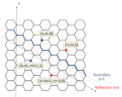
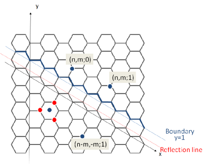
$(a)$	$(b)$

Figure 2: Principal boundary with closed $(a)$ and open $(b)$ boundary condition.

For the closed boundary condition, each site of the half-plane above or on the boundary is mirrored through the reflection line shown as the dotted red line. An $A$-site has a mirror image which is a $B$-site and vice-versa. The coordinates of the images are indicated in Fig.2a. The closed Green function for the principal boundary then reads

$$G_{(n_{1},m_{1};\alpha)(n_{2},m_{2};0)}^{\rm cl} \!\!\!=\!\!\! G_{(n_{1},m_{1};\alpha)(n_{2},m_{2};0)}+G_{(n_{1},m_{1};\alpha)(n_{2}-m_{2},1-m_{2};1)},$$ (4.8)

$$G_{(n_{1},m_{1};\alpha)(n_{2},m_{2};1)}^{\rm cl} \!\!\!=\!\!\! G_{(n_{1},m_{1};\alpha)(n_{2},m_{2};1)}+G_{(n_{1},m_{1};\alpha)(n_{2}-m_{2}+1,1-m_{2};0)}.$$ (4.9)

For the open boundary condition, the situation is slightly more complicated. The reflection line, shown in Fig.2b as the dotted red line, is such that a $B$-site above the boundary reflects itself to a $B$-site below the boundary, however the mirror image of an $A$-site does not belong to the lattice. Instead the strict mirror of an $A$-site is the center of an hexagon lying below the boundary. We then define the three $B$-sites on this hexagon as the three mirror images of the $A$-site above the boundary, each one being weighted by a factor $1/3$. The open Green function is then related to the Green function on the plane by the following expressions,

$$G_{(n_{1},m_{1};\alpha)(n_{2},m_{2};0)}^{\rm op} \!\!\!=\!\!\! G_{(n_{1},m_{1};\alpha)(n_{2},m_{2};0)}-\frac{1}{3}\Big{[}G_{(n_{1},m_{1};\alpha)(n_{2}-m_{2},-m_{2};1)}+$$ (4.10)

$$\hskip 28.45274pt+\>G_{(n_{1},m_{1};\alpha)(n_{2}-m_{2}-1,-m_{2};1)}+G_{(n_{1},m_{1};\alpha)(n_{2}-m_{2},-m_{2}+1;1)}\Big{]},$$

$$G_{(n_{1},m_{1};\alpha)(n_{2},m_{2};1)}^{\rm op} \!\!\!=\!\!\! G_{(n_{1},m_{1};\alpha)(n_{2},m_{2};1)}-G_{(n_{1},m_{1};\alpha)(n_{2}-m_{2},-m_{2};1)}.$$ (4.11)

These formulas and the asymptotic behaviour of the bulk Green function enable us to obtain the asymptotic behaviour of $G^{\rm op}$ and $G^{\rm cl}$, and in turn, the scaling form of the height 1 probabilities. The height $1$ probability at an arbitrary point $(n,m;\alpha)$ does not depend on $n$, by translational invariance along the $\hat{n}$ axis. When $m\gg 1$ and for $\alpha=0$, we obtain the following 1-site probabilities,

$$P_{1}^{\rm op}(m)-P_{1} \!\!\!=\!\!\! +\frac{1}{12\sqrt{3}\pi}\frac{1}{m^{2}}+\frac{1}{18\sqrt{3}\pi}\frac{1}{m^{3}}+\ldots=+\frac{\sqrt{3}P_{1}}{\pi}\frac{1}{4r^{2}}+\ldots,$$ (4.12)

$$P_{1}^{\rm cl}(m)-P_{1} \!\!\!=\!\!\! -\frac{1}{12\sqrt{3}\pi}\frac{1}{m^{2}}-\frac{1}{9\sqrt{3}\pi}\frac{1}{m^{3}}+\ldots=-\frac{\sqrt{3}P_{1}}{\pi}\frac{1}{4r^{2}}+\ldots$$ (4.13)

where $r=\sqrt{3}(m-1)/2$ is the Euclidean distance from the site $(n,m;0)$ to the boundary. The distinctive change of sign between the two types of boundary conditions was also found on the square lattice [9, 5].

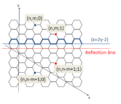
Figure 3: Horizontal boundary with the open boundary condition.

Let us now look at the second, horizontal boundary, shown in Fig.3. We try to adapt the image method to this boundary in order to compute the discrete Green function for open and closed boundary. For the open condition, the image points are found by a reflection with respect to the horizontal line $n=2m-1$, pictured as the dotted red line in Fig.3. Such a reflection preserves the type, $A$ or $B$, of sites, so that we obtain

$$G_{(n_{1},m_{1};\alpha)(n_{2},m_{2};\beta)}^{\rm op}=G_{(n_{1},m_{1};\alpha)(n_{2},m_{2};\beta)}-G_{(n_{1},m_{1};\alpha)(n_{2},n_{2}-m_{2}+1;\beta)}.$$ (4.14)

In contrast, for the closed boundary condition, we have not been able to define the appropriate reflection map, with one mirror image or several mirror images like above, so as to make the image method work. As a consequence, we could compute the 1-site height 1 probability for the open condition only. The probability for finding a height $1$ at a site $(2y-2,y+m-1;\alpha)$, located at a distance $r=m-1$ from the horizontal boundary, does not depend on $y$. So we may put $y=1$ and consider the site $(0,m;\alpha)$, in which case the probability reads

$$P_{1}^{\rm op}(m)-P_{1}=+\frac{1}{16\sqrt{3}\pi}\frac{1}{m^{2}}+\ldots=+\frac{\sqrt{3}P_{1}}{\pi}\frac{1}{4r^{2}}+\dots$$ (4.15)

with the same dominant term as for the other boundary, as expected.

4.3 On boundaries

Finally the height $1$ correlation functions along a boundary can be computed for the types of boundaries considered above. In each case, a boundary site has only two neighbours so that the defect matrix required to force a height 1 is two-by-two and depends on the boundary condition, open or closed. Explicitly they read

$$B^{\rm op}=\pmatrix{-2&1\cr 1&-1},\qquad B^{\rm cl}=\pmatrix{-1&1\cr 1&-1}.$$ (4.16)

On the principal boundary, it is not difficult, with the appropriate Green functions given in the previous subsection, to compute the one-site probabilities for a height 1, on an open or a closed boundary,

$$P_{1}^{\rm op}=\frac{11}{36}+\frac{4}{\sqrt{3}\pi}-\frac{9}{\pi^{2}}\simeq 0.129,\qquad P_{1}^{\rm cl}=\frac{\sqrt{3}}{\pi}-\frac{1}{3}\simeq 0.218.$$ (4.17)

We note that the height of a closed site can only take the values 1 and 2, so that the previous result implies $P_{2}^{\rm cl}={4\over 3}-{\sqrt{3}\over\pi}\simeq 0.782$.

For the joint probabilities of having two, three or four heights 1 separated by distances $r_{ij}$ along the principal boundary, we obtain, for the open boundary condition,

$$P^{\rm op}_{11}\Big{|}_{\rm conn}=-{1\over 4}\Big{(}{11\over 2\sqrt{3}\pi}-{9\over\pi^{2}}\Big{)}^{2}{1\over r_{12}^{4}}+\ldots$$ (4.18)

$$P^{\rm op}_{111}\Big{|}_{\rm conn}=-{1\over 4}\Big{(}{11\over 2\sqrt{3}\pi}-{9\over\pi^{2}}\Big{)}^{3}{1\over(r_{12}r_{13}r_{23})^{2}}+\ldots$$ (4.19)

$$P^{\rm op}_{1111}\Big{|}_{\rm conn}=-{1\over 8}\Big{(}{11\over 2\sqrt{3}\pi}-{9\over\pi^{2}}\Big{)}^{4}\left\{{1\over(r_{12}r_{13}r_{24}r_{34})^{2}}+{1\over(r_{12}r_{14}r_{23}r_{34})^{2}}+{1\over(r_{13}r_{14}r_{23}r_{24})^{2}}\right\}$$

$$\hskip 227.62204pt+\ldots$$ (4.20)

and similar expressions for the closed boundary condition,

$$P^{\rm cl}_{11}\Big{|}_{\rm conn}=-{1\over 4}\Big{(}{\sqrt{3}\over 2\pi}\Big{)}^{2}{1\over r_{12}^{4}}+\ldots$$ (4.21)

$$P^{\rm cl}_{111}\Big{|}_{\rm conn}={1\over 4}\Big{(}{\sqrt{3}\over 2\pi}\Big{)}^{3}{1\over(r_{12}r_{13}r_{23})^{2}}+\ldots$$ (4.22)

$$P^{\rm cl}_{1111}\Big{|}_{\rm conn}=-{1\over 8}\Big{(}{\sqrt{3}\over 2\pi}\Big{)}^{4}\left\{{1\over(r_{12}r_{13}r_{24}r_{34})^{2}}+{1\over(r_{12}r_{14}r_{23}r_{34})^{2}}+{1\over(r_{13}r_{14}r_{23}r_{24})^{2}}\right\}+\ldots\quad$$ (4.23)

On the horizontal boundary, and for the open boundary condition only (as explained above, we cannot handle the closed condition), we obtain similar results for the single site height 1 probability,

$$P_{1}^{\rm op}=-\frac{37}{36}+\frac{8}{\sqrt{3}\pi}-\frac{3}{\pi^{2}}\simeq 0.1385,$$ (4.24)

and for the first correlation functions,

$$P^{\rm op}_{11}\Big{|}_{\rm conn}=-{1\over 4}\Big{(}{1\over\pi^{2}}-{\sqrt{3}\over 9\pi}\Big{)}^{2}{1\over r_{12}^{4}}+\ldots$$ (4.25)

$$P^{\rm op}_{111}\Big{|}_{\rm conn}=-{1\over 4}\Big{(}{1\over\pi^{2}}-{\sqrt{3}\over 9\pi}\Big{)}^{3}{1\over(r_{12}r_{13}r_{23})^{2}}+\ldots$$ (4.26)

$$P^{\rm op}_{1111}\Big{|}_{\rm conn}=-{1\over 8}\Big{(}{1\over\pi^{2}}-{\sqrt{3}\over 9\pi}\Big{)}^{4}\left\{{1\over(r_{12}r_{13}r_{24}r_{34})^{2}}+{1\over(r_{12}r_{14}r_{23}r_{34})^{2}}+{1\over(r_{13}r_{14}r_{23}r_{24})^{2}}\right\}$$

$$\hskip 227.62204pt+\ldots$$ (4.27)

5 Conformal Field Theory

If the above results for heights 1 on the honeycomb lattice are compared with those obtained on the square lattice [5, 6, 15, 16], it is immediately clear that they coincide, up to normalizations, and thereby confirm the universality of the field assignements. So we restrict here to a brief reminder of the main features of the conformal field interpretation of these lattice results, and take the opportunity to collect the various formulas.

On the square lattice, it has been shown that, in the scaling limit, i.e. in the large distance limit, the joint height 1 probabilities on the lattice are exactly reproduced by conformal correlators of primary fields. If the height 1 variable lives in the bulk, the corresponding primary field is a non-chiral field with conformal weights $(1,1)$, whereas it is a chiral, boundary primary field of weight 2 in the case the height 1 lies on a boundary, closed or open. It turns out that all these correlators can be understood, and computed, by writing the primary fields in terms of a pair of symplectic free fermions $\theta,\tilde{\theta}$.

The theory of symplectic free fermions, with central charge $c=-2$, is the logarithmic conformal field theory which is, by far, the best understood, see for instance [30], and the more recent work [31] as well as the references therein. We only need here the most basic features of it.

The symplectic fermions are anticommuting, space-time scalar fields with propagators given by

$$\mbox{\hskip 3.99994pt}\vtop{\halign{#\cr$\hfil\displaystyle{\mbox{}\theta(z,\bar{z})\theta}\hfil\mbox{}$\crcr\kern-1.9pt\nointerlineskip\vskip 2.0pt\cr$\mathord{{\vrule height=5.0pt,width=0.4pt,depth=0.0pt}}\hrulefill\mathord{{\vrule height=5.0pt,width=0.4pt,depth=0.0pt}}$\crcr}}\mbox{\hskip 3.99994pt}(w,\bar{w}) \!\!\!=\!\!\! \mbox{\hskip 3.99994pt}\vtop{\halign{#\cr$\hfil\displaystyle{\mbox{}\tilde{\theta}(z,\bar{z})\tilde{\theta}}\hfil\mbox{}$\crcr\kern-1.9pt\nointerlineskip\vskip 2.0pt\cr$\mathord{{\vrule height=5.0pt,width=0.4pt,depth=0.0pt}}\hrulefill\mathord{{\vrule height=5.0pt,width=0.4pt,depth=0.0pt}}$\crcr}}\mbox{\hskip 3.99994pt}(w,\bar{w})=0,$$ (5.5)

$$\mbox{\hskip 3.99994pt}\vtop{\halign{#\cr$\hfil\displaystyle{\mbox{}\theta(z,\bar{z})\tilde{\theta}}\hfil\mbox{}$\crcr\kern-1.9pt\nointerlineskip\vskip 2.0pt\cr$\mathord{{\vrule height=5.0pt,width=0.4pt,depth=0.0pt}}\hrulefill\mathord{{\vrule height=5.0pt,width=0.4pt,depth=0.0pt}}$\crcr}}\mbox{\hskip 3.99994pt}(w,\bar{w}) \!\!\!=\!\!\! -\log{|z-w|},$$ (5.8)

from which all higher correlators may be obtained from Wick’s theorem. Since the propagator (5.8) is a sum of a chiral term and a antichiral term, the fermions satisfy $\partial\bar{\partial}\theta=\partial\bar{\partial}\tilde{\theta}=0$ in all correlators. A Langrangean realization is provided by the action $S\sim\int\partial\theta\bar{\partial}\tilde{\theta}$, which has the previous two conditions as equations of motion.

The fermion fields themselves are not primary, but their first derivatives are primary. In particular $\phi(z,\bar{z})=\partial\bar{\partial}(\theta\tilde{\theta})$ is a primary field with conformal weights $(1,1)$. It is not difficult to compute its 2-, 3- and 4-point functions. They are given explicitly by the following expressions where $z_{ij}=z_{i}-z_{j}$,

$$\langle\phi(1)\phi(2)\rangle=-{1\over 2|z_{12}|^{4}},$$ (5.9)

$$\langle\phi(1)\phi(2)\phi(3)\rangle=0,$$ (5.10)

$$\langle\phi(1)\phi(2)\phi(3)\phi(4)\rangle={1\over 4|z_{12}z_{34}|^{4}}+{1\over 4|z_{13}z_{24}|^{4}}+{1\over 4|z_{14}z_{23}|^{4}}$$

$$\hskip 71.13188pt-{1\over 8}\left\{{1\over(z_{12}z_{34}\bar{z}_{13}\bar{z}_{24})^{2}}+{1\over(z_{13}z_{24}\bar{z}_{14}\bar{z}_{23})^{2}}+{1\over(z_{14}z_{23}\bar{z}_{12}\bar{z}_{34})^{2}}+{\rm c.c.}\right\}.$$ (5.11)

The 3-correlator vanishes identically because the various Wick contractions necessarily involve the contraction of $\partial\theta$ with $\bar{\partial}\tilde{\theta}$, or $\bar{\partial}\theta$ with $\partial\tilde{\theta}$. In the 4-point correlator, the first three terms are products of 2-point functions and are not part of the connected correlator.

The correlation functions of $\phi$ on the upper-half plane can be similarly computed by using the appropriate Green function, namely

$$\mbox{\hskip 3.99994pt}\vtop{\halign{#\cr$\hfil\displaystyle{\mbox{}\theta(z,\bar{z})\tilde{\theta}}\hfil\mbox{}$\crcr\kern-1.9pt\nointerlineskip\vskip 2.0pt\cr$\mathord{{\vrule height=5.0pt,width=0.4pt,depth=0.0pt}}\hrulefill\mathord{{\vrule height=5.0pt,width=0.4pt,depth=0.0pt}}$\crcr}}\mbox{\hskip 3.99994pt}(w,\bar{w})=-\log{|z-w|}\pm\log{|z-\bar{w}|},$$ (5.12)

with the $+$ sign for the closed boundary, and the $-$ sign for the open boundary. It yields in particular the 1-point function of $\phi$ on the upper-half plane,

$$\langle\phi(z,\bar{z})\rangle_{\rm cl\atop op}=\pm{1\over 4({\rm Im}\,z)^{2}}.$$ (5.13)

A simple comparison with the results obtained in the previous section shows that the leading terms of the connected joint probabilities are exactly reproduced by the above correlators provided the subtracted height 1 variable $\delta(h_{i}-1)-P_{1}$ converges, in the scaling limit, to $\alpha\phi(z,\bar{z})$ for some normalization $\alpha$. The results in the bulk imply that for the honeycomb lattice, $\alpha=\pm{\sqrt{3}P_{1}\over\pi}$. The results on the upper-half planes then fix the sign,

$$\alpha^{\rm h.c.}=-{\sqrt{3}P_{1}^{\rm h.c.}\over\pi}=-{1\over 4\sqrt{3}\pi}.$$ (5.14)

By comparison, the results for the square lattice imply $\alpha^{\rm sq}=-P_{1}^{\rm sq}=-{2(\pi-2)\over\pi^{3}}$ [5]. The way this specific conformal field emerges in the scaling limit has been demonstrated in [22]. Moreover, from the conformal field theory point of view, the open and closed boundary conditions have been shown [7] to be related to each other by the insertion of a chiral primary field of conformal weight $-1/8$, and leads to the change of sign in the 1-point function of $\phi$ on the upper-half plane.

For the purpose of describing the boundary height 1, we need the chiral version of the previous fields. So one also considers chiral symplectic free fermions with contractions

$$\mbox{\hskip 3.99994pt}\vtop{\halign{#\cr$\hfil\displaystyle{\mbox{}\theta(z)\theta}\hfil\mbox{}$\crcr\kern-1.9pt\nointerlineskip\vskip 2.0pt\cr$\mathord{{\vrule height=5.0pt,width=0.4pt,depth=0.0pt}}\hrulefill\mathord{{\vrule height=5.0pt,width=0.4pt,depth=0.0pt}}$\crcr}}\mbox{\hskip 3.99994pt}(w) \!\!\!=\!\!\! \mbox{\hskip 3.99994pt}\vtop{\halign{#\cr$\hfil\displaystyle{\mbox{}\tilde{\theta}(z)\tilde{\theta}}\hfil\mbox{}$\crcr\kern-1.9pt\nointerlineskip\vskip 2.0pt\cr$\mathord{{\vrule height=5.0pt,width=0.4pt,depth=0.0pt}}\hrulefill\mathord{{\vrule height=5.0pt,width=0.4pt,depth=0.0pt}}$\crcr}}\mbox{\hskip 3.99994pt}(w)=0,$$ (5.19)

$$\mbox{\hskip 3.99994pt}\vtop{\halign{#\cr$\hfil\displaystyle{\mbox{}\theta(z)\tilde{\theta}}\hfil\mbox{}$\crcr\kern-1.9pt\nointerlineskip\vskip 2.0pt\cr$\mathord{{\vrule height=5.0pt,width=0.4pt,depth=0.0pt}}\hrulefill\mathord{{\vrule height=5.0pt,width=0.4pt,depth=0.0pt}}$\crcr}}\mbox{\hskip 3.99994pt}(w) \!\!\!=\!\!\! -{1\over 2}\log{(z-w)}.$$ (5.22)

The chiral version of $\phi$ that we will use, namely $\phi_{\rm c}=\partial\theta\partial\tilde{\theta}$, is not a primary field since it is proportional to the stress-energy tensor of the Lagrangean realization, $T(z)=2\,\partial\theta\partial\tilde{\theta}$. The first correlators of $\phi_{\rm c}$ with itself read

$$\langle\phi_{\rm c}(1)\phi_{\rm c}(2)\rangle=-{1\over 4z_{12}^{4}},$$ (5.23)

$$\langle\phi_{\rm c}(1)\phi_{\rm c}(2)\phi_{\rm c}(3)\rangle=-{1\over 4}{1\over(z_{12}z_{13}z_{23})^{2}},$$ (5.24)

$$\langle\phi_{\rm c}(1)\phi_{\rm c}(2)\phi_{\rm c}(3)\phi_{\rm c}(4)\rangle={1\over 16(z_{12}z_{34})^{4}}+{1\over 16(z_{13}z_{24})^{4}}+{1\over 16(z_{14}z_{23})^{4}}$$

$$\hskip 71.13188pt-{1\over 8}\left\{{1\over(z_{12}z_{13}z_{24}z_{34})^{2}}+{1\over(z_{12}z_{14}z_{23}z_{34})^{2}}+{1\over(z_{13}z_{14}z_{23}z_{24})^{2}}\right\}.$$ (5.25)

The boundary 2-, 3- and 4-correlators computed in Section 4.3 have exactly these functional forms, and show that the boundary height 1 variable, subtracted with the appropriate value of $P_{1}$, converges to $\alpha_{\rm c}\,\phi_{\rm c}$. The normalization depends on the type of boundary, principal or horizontal, and on the boundary condition. One finds

$$\alpha_{\rm c}^{\rm h.c.,princ,op}={11\over 2\sqrt{3}\pi}-{9\over\pi^{2}},\quad\quad\alpha_{\rm c}^{\rm h.c.,princ,cl}=-{\sqrt{3}\over 2\pi},$$ (5.26)

$$\alpha_{\rm c}^{\rm h.c.,horiz,op}={1\over\pi^{2}}-{\sqrt{3}\over 9\pi}.$$ (5.27)

The two normalization factors for the open condition are positive, whereas the normalization for the closed condition is negative.

On the square lattice, the boundary height 1 variable was also seen to converge to $\phi_{\rm c}$ with a normalization, on a boundary parallel to a principal axis, given by [15, 16]

$$\alpha_{\rm c}^{\rm sq,op}={6\over\pi}-{160\over 3\pi^{2}}+{1024\over 9\pi^{3}},\quad\quad\alpha_{\rm c}^{\rm sq,cl}=-{8\over\pi}\Big{(}{3\over 4}-{2\over\pi}\Big{)}.$$ (5.28)

Again the normalization is positive for the open, and negative for the closed boundary condition.

It should be emphasized that, whereas the scaling limit of the height 1 variables, in the bulk and on open/closed boundaries, can be described by conformal fields which are themselves related in a simple way to symplectic free fermions, it is not so for all observables of the sandpile model.

On the square lattice, it has been shown that boundary higher height variables scale to conformal fields which have simple expressions in terms of symplectic fermions. On an open boundary, the heights 2, 3 and 4 scale to the same field $\phi_{\rm c}$ as the height 1, while the heights 2 and 3 on a closed boundary have a slightly different scaling, since they converge to a combination of $\phi_{\rm c}$ and $\theta\partial\partial\tilde{\theta}$. On the honeycomb lattice, only the field $\phi_{c}$ is expected (a closed site has two neighbours, and therefore its height takes only two values).

In contrast, the higher height variables in the bulk are all described, up to normalization, by a single scaling field $\psi$, which turns out to be a logarithmic partner of the field $\phi$ describing the height 1 in the bulk. However the reducible but indecomposable representation they generate does not belong to the theory of symplectic fermions. Whether this representation has a Lagrangean realization is an open and important problem. The same distinction between the height 1 and the higher heights in the bulk is expected on the honeycomb lattice, or indeed on any regular lattice.

6 Boundary of Wave Clusters and Conformal Invariance

The scaling behaviour of the two-dimensional critical lattice models can be reflected in the statistics of non-crossing random curves which form the boundaries of clusters on the lattice. In the 1920’s, Loewner studied simple curves growing from the origin into the upper-half plane ${H}$ [33]. Loewner’s idea was to describe the evolution of these curves in terms of the evolution of the analytic function $g_{t}$, which maps conformally the region outside of the curve into ${H}$. He showed that this function satisfies the following differential equation

$$\frac{dg_{t}(z)}{dt}=\frac{2}{g_{t}(z)-\xi_{t}},$$ (6.1)

for a real continuous function $\xi_{t}$, related to the image of the tip of the curve under $g_{t}$. Conversely, a continuous real function $\xi_{t}$ implicitly defines a curve growing in ${H}$.

Much more recently, Schramm followed the idea that a measure on the continuous driving functions $\xi_{t}$ would induce a measure on the set of growing curves in ${H}$, and showed that the latter measure is conformally invariant if and only if the former measure is the Wiener measure for the standard one-dimensional Brownian motion $B_{t}$ [34]. This subsequently led to a completely new perspective on random curves arising in conformally invariant critical systems, see [35] for a review. In this context, setting $\xi_{t}=\sqrt{\kappa}B_{t}$ for different parameter $\kappa$ corresponds to different universality classes of critical behaviour.

Avalanche boundaries in Abelian sandpile model are random dynamical curves whose statistics can be studied using the theory of SLE [27]. It has been suggested, on the basis of numerical simulations on the square lattice, that the boundaries of avalanche clusters are conformally invariant with the same properties as loop erased random walk model, with diffusivity constant $\kappa=2$.

Since an avalanche has a complicated structure, understanding its dynamics can be simplified by decomposing the avalanche into a sequence of more elementary objects called toppling waves [18]. The waves are constructed as follows. If, as a result of the addition of a grain to a site $i$, that site $i$ becomes unstable, it topples, as do the sites which become unstable as a consequence of the first toppling at $i$. The first wave is the collection of all sites which have toppled given that the initial site is not allowed to topple more than once. One can show that the sites in the first wave all topple exactly once. After the first wave is completed, the initial site, if still unstable, is allowed to topple a second time, and doing so, triggers the second wave of topplings. The process continues, with a third wave, fourth wave and so on, until the initial site $i$ is stable and the avalanche stops. The important property of waves is that they are individually compact (no hole), and the sites in each wave topple exactly once.

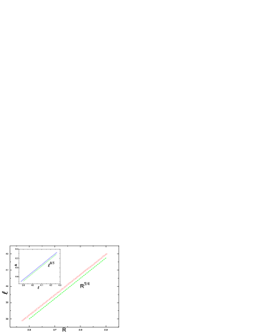
Figure 4: Main frame: Log-log plot of the length of wave boundaries $l$ versus the radius of gyration $R$, simulated on the honeycomb lattice with the linear size of $2048$. Inset: Log-log plot of the average area of wave clusters $A$ versus the length $l$.

To check the universality of the model, we consider an ensemble of wave boundaries, on the honeycomb lattice, and repeat the analysis carried out in [27] for the square lattice. At first, we calculate the fractal dimension $d_{f}$ for the wave boundaries, determined by the scaling relation $l\sim R^{d_{f}}$ between the perimeter $l$ of the curve and the radius of gyration $R$. The result for waves is $d_{f}=1.25\pm 0.01$, see Fig. 4. The inset of Fig. 4 shows the scaling of the mean area of the wave clusters with their perimeter length as $A\sim l^{2/d_{f}}$, which is consistent with the one discussed in [36]. Furthermore, from the relation $d_{f}=1+\frac{\kappa}{8}$ for the fractal dimension of SLE curves [37], this fractal dimension is consistent with the value $\kappa=2$, obtained for the boundary of avalanche clusters on the square lattice [27]. The central charge associated with $\kappa=2$ is $c={(3\kappa-8)(6-\kappa)\over 2\kappa}=-2$ [38].

One of the questions about SLE curves that has a neat answer is the following: for a curve connecting two points on the boundary of a domain $D$, what is the probability that the curve passes to the left of a given point interior to the domain ? It is usual to take the domain $D$ to be the upper-half plane and the boundary points to be the origin and the point at infinity. In this case, an interior point of the domain is represented in polar coordinates as $z=Re^{i\phi}$. By scale invariance, the above probability depends only on $\phi\in[0,\pi]$ and is given by [39]

$$P_{\kappa}(\phi)=\frac{1}{2}+\frac{\Gamma(\frac{4}{\kappa})}{\sqrt{\pi}\Gamma(\frac{8-\kappa}{2\kappa})}F_{12}\left(\frac{1}{2};\frac{4}{\kappa};\frac{3}{2};-\cot^{2}(\phi)\right)\cot(\phi),$$ (6.2)

where $F_{12}$ is the hypergeometric function. For $k=2$, this reduces to

$$P_{2}(\phi)=1-{2\phi-\sin{2\phi}\over 2\pi}.$$ (6.3)

In order to check Eq.(6.3) for wave curves (loop curves), at first step we should convert these curves to curves which connect the origin to the infinity (chordal SLE). To this aim, we cross any given loop by an arbitrary straight line as real line at two points $x_{0}=0$ and $x_{\infty}$ and consider only a segment of curve which is above the real line. Then by the conformal map $\varphi(z)=\frac{x_{\infty}z}{x_{\infty}-z}$, curves in the upper half plane are transformed to a set of curves connecting the origin to infinity.
The computed probabilities for points at distances $R=0.1,0.2,0.4$ and $0.5$ is consistent with Eq.(6.2), with $\kappa=2.1\pm 0.1$ (see Fig. 5 (a)).

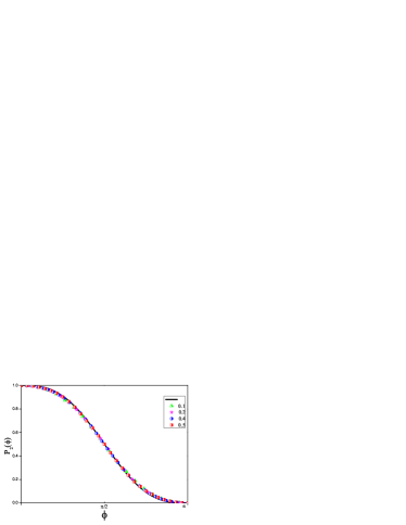
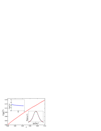
$(a)$	$(b)$

Figure 5: $(a)$ The probability that a wave boundary passes to the left of a point with polar coordinates $(R,\phi)$, for $R=0.1,0.2,0.4$ and $0.5$. The solid line shows the function $P_{2}(\phi)$ obtained from SLE for $\kappa=2$. $(b)$ Statistics of the driving function $\xi(t)$ for the wave boundaries in the sandpile model on the honeycomb lattice. Main frame: the linear behaviour of $\langle\xi(t)^{2}\rangle$ with the slope $\kappa=2.0\pm 0.2$. Upper-right inset: the diffusion coefficient is $\kappa=2.0\pm 0.2$. Lower-left inset: the probability distribution function of the noise $\xi(t)/\sqrt{\kappa t}$, different colors correspond to $t=0.02,0.04,0.06,0.08.$

A more careful test which shows the correspondence with SLE, is to extract the Loewner driving function $\xi_{t}$. There is an algorithm for chordal SLE curves, based on the approximation that driving function is a piecewise constant function [40]. As we mentioned at previous case, with conformal map $\varphi(z)=\frac{x_{\infty}z}{x_{\infty}-z}$, the segment of loop curves at upper half plane are converted to chordal curves. Then, each curve is parameterized by the dimensionless parameter $t$ (that it is not time). In this case the Lowener equation is as $dg_{t}/dt=2/\{\varphi^{\prime}(g_{t})[\varphi(g_{t})-\xi_{t}]\}$, which $g_{t}(z)$ maps the half-plane minus the curve up to $t$ into the whole of upper half-plane. For a constant $\xi$, the equation can be solved for $g_{t}$ as:

$$G_{t,\xi}(z)=x_{\infty}{\eta x_{\infty}(x_{\infty}-z)+\sqrt{x_{\infty}^{4}(z-\eta)^{2}+4t(x_{\infty}-z)^{2}\times(x_{\infty}-\eta)^{2}}\over x_{\infty}^{2}(x_{\infty}-z)+\sqrt{x_{\infty}^{4}(z-\eta)^{2}+4t(x_{\infty}-z)^{2}\times(x_{\infty}-\eta)^{2}}}$$ (6.4)

Where, $\eta=\varphi^{-1}(\xi)$.
According to algorithm, the interval $[0,T]$ is divided to smaller intervals $[t_{n},t_{n+1})$ with $t_{0}=0$ and $t_{N+1}=T$, such that the $\xi(t)$ is approximated by the constant $\xi_{n}=\xi(t_{n})$ in each interval. In this case, the function of $g_{t}$ is expressed as composition of $G_{t_{N}-t_{N-1},\xi_{N-1}}o\ldots oG_{t_{1},\xi_{0}}$. The action of each of $G_{t,\xi}(z)$ is such that when they apply on the points of the curve, remove the first point from the sequence of points.
Now, we follow this algorithm for extracting of the driving function. At First, we take the points of our curves on upper half plane approximated with $\{z_{0}=0,z_{1},\ldots,z_{N}=x_{\infty}\}$. Then, using the parameters $\eta_{0}=\varphi^{-1}(\xi_{0})=[Rez_{1}x_{\infty}-(Rez_{1})^{2}-(Imz_{1})^{2}]/(x_{\infty}-Rez_{1})$ and $t_{1}=(Imz_{1})^{2}x_{\infty}^{4}/\{4[(Rez_{1}-x_{\infty})^{2}+(Imz_{1})^{2}]^{2}\}$,the map $G_{t_{1},\xi_{0}}$ applied to the points resulting in a new sequence, by one element shorter: $z^{\prime}_{k}=G_{t_{1},\xi_{0}}(z_{k+1})$, with $k=1,\ldots,N$. The operation is iterated on the new subsequence of points until one obtains the full set of $t_{k}$ and $\xi_{k}$ for each curve. The result of this procedure is an ensemble of $\xi(t)$ that its statistics as shown in Fig. 5 (b) ,converges to a Gaussian process with variance $\langle\xi^{2}(t)\rangle=\kappa t$ and $\kappa=2.0\pm 0.2$. This result, together with the other evidences, certify that the wave boundary curves of sandpile model are conformally invariant and described by the SLE₂.
This result seems to be reasonable from the correspondence with the spanning trees. In fact, one can construct exactly a two-component tree on the lattice, representing a wave [18]. The boundary of a wave as the dual of the spanning tree is expected to be SLE₂. The statistics of the wave boundaries with diffusion coefficient $\kappa=2$ confirm the relation of the sandpile model with a $c=-2$ conformal field theory.

7 Conclusions

In this paper, we have investigated some of the properties of the Abelian sandpile model on the honeycomb lattice. The scaling behaviours of the height correlation functions in the bulk, in the presence of boundaries, and on boundaries, are in the agreement with those obtained on the square lattice, and correctly predicted by a $c=-2$ conformal field theory.

We have also checked the universality properties of the model from the point of view of its geometrical features, namely the statistics of the boundaries of the toppling waves. We found numerically that the boundaries of wave clusters are conformally invariant, and well described by the SLE process with diffusivity $\kappa=2$.

Appendix A Appendix

We collect in this Appendix some of the values of the lattice Green function on the honeycomb lattice, for small distances, and also give its asymptotic behaviour for large distances.

In the coordinate system used in Section 2, the Green function on the honeycomb lattice for a pair of points of the $A$ type and separated by the vector $(n,m)$, is given by

$$G_{AA}(n,m)={3\over 8\pi^{2}}\int\!\!\!\!\int_{-\pi}^{\pi}\;{\rm d}\theta_{1}\,{\rm d}\theta_{2}\>{e^{in\theta_{1}+im\theta_{2}}\over 3-\cos{\theta_{1}}-\cos{\theta_{2}}-\cos{(\theta_{1}+\theta_{2})}}.$$ (A.1)

One of the two integrations can be carried out, and leads to the following result [41]

$$G_{AA}(n,m)={3\over 2\pi}\int_{0}^{\pi/2}\;{\rm d}x\>{e^{-|n-m|s}\cos{(n+m)x}\over\sin{x}\,\sqrt{4-\cos^{2}{x}}},$$ (A.2)

where the function $s(x)$ is defined through

$$\sinh{s}={\sin{x}\over\cos{x}}\,\sqrt{4-\cos^{2}{x}}.$$ (A.3)

The previous integral is still divergent, but provides a convergent integral representation for the subtracted Green function $\Phi_{AA}(n,m)\equiv G_{AA}(n,m)-G_{AA}(0,0)$. It yields the following values for small $n,m$ [42],

$$\Phi_{AA}(1,0) \!\!\!=\!\!\! \Phi_{AA}(1,1)=-{1\over 2},$$ (A.4)

$$\Phi_{AA}(1,2) \!\!\!=\!\!\! \Phi_{AA}(-1,1)=1-{3\sqrt{3}\over\pi},$$ (A.5)

$$\Phi_{AA}(2,0) \!\!\!=\!\!\! \Phi_{AA}(2,2)=-4+{6\sqrt{3}\over\pi},$$ (A.6)

$$\Phi_{AA}(2,3) \!\!\!=\!\!\! \Phi_{AA}(-1,2)={15\over 2}-{15\sqrt{3}\over\pi},$$ (A.7)

$$\Phi_{AA}(3,0) \!\!\!=\!\!\! \Phi_{AA}(3,3)=-{81\over 2}+{72\sqrt{3}\over\pi}.$$ (A.8)

Let us now evaluate the asymptotic behaviour of $\Phi_{AA}(n,m)$ for large distances. We will do this calculation by using ideas from [41] and [13]; the analogous calculation for the square lattice has been done in [43].

The basic idea underlying these computations is that for large $|n-m|$, the exponential factor in (A.2) contributes significantly only in the region where $s$ is small, which is also where $x$ is small. In this region, we may expand $s(x)$ in powers of $x$,

$$s(x)=\sqrt{3}\Big{(}x+{2\over 45}x^{5}+{2\over 405}x^{9}+\ldots\Big{)}.$$ (A.9)

Therefore the main contribution of the integral comes from the part close to the origin and is given by the way the rest of the integrand behaves for small $x$.

We start by splitting the integral giving $\Phi_{AA}(n,m)$ into three pieces,

$$\Phi_{AA}(n,m) \!\!\!=\!\!\! {3\over 2\pi}\int_{0}^{\pi/2}\;{\rm d}x\>{e^{-|n-m|s}\cos{(n+m)x-1}\over\sin{x}\,\sqrt{4-\cos^{2}{x}}}$$ (A.10)

$$=\;{3\over 2\pi}\int_{0}^{\pi/2}\;{\rm d}x\>\Big{\{}{e^{-|n-m|s}\cos{(n+m)x}\over\sin{x}\,\sqrt{4-\cos^{2}{x}}}-{e^{-\sqrt{3}|n-m|x}\cos{(n+m)x}\over\sqrt{3}x}\Big{\}}$$

$$+\;{3\over 2\pi}\int_{0}^{\pi/2}\;{\rm d}x\>\Big{\{}{e^{-\sqrt{3}|n-m|x}\cos{(n+m)x}\over\sqrt{3}x}-{1\over\sqrt{3}x}\Big{\}}$$

$$+\;{3\over 2\pi}\int_{0}^{\pi/2}\;{\rm d}x\>\Big{\{}{1\over\sqrt{3}x}-{1\over\sin{x}\,\sqrt{4-\cos^{2}{x}}}\Big{\}}.$$

The second integral can be evaluated exactly, up to exponentially small terms, and turns out to give the dominant, logarithmic term, equal to $-{\sqrt{3}\over 2\pi}(\log{r}+\gamma+\log{\pi})$, where $r^{2}=n^{2}+m^{2}-nm$ and $\gamma=0.577216$ is the Euler constant. The third integral is a constant which can also be computed exactly, and is equal to ${\sqrt{3}\over 4\pi}\log{\pi^{2}\over 12}$. We obtain at this stage

$$\Phi_{AA}(n,m) \!\!\!=\!\!\! -{\sqrt{3}\over 2\pi}\left[\log{r}+\gamma+{1\over 2}\log{12}\right]$$ (A.11)

$$\!\!\!+\!\!\! {3\over 2\pi}\int_{0}^{\pi/2}\;{\rm d}x\>\Big{\{}{e^{-|n-m|s}\cos{(n+m)x}\over\sin{x}\,\sqrt{4-\cos^{2}{x}}}-{e^{-\sqrt{3}|n-m|x}\cos{(n+m)x}\over\sqrt{3}x}\Big{\}}.$$

To evaluate the remaining integral, we use the expansion of $s$ as a power series in $x$, and write $e^{-|n-m|s}=e^{-\sqrt{3}|n-m|x}Q(x)$ where $Q$ is expanded as

$$Q(x)=\exp{[-|n-m|(s-\sqrt{3}x)]}=\exp{\Big{\{}-\sqrt{3}|n-m|\Big{(}{2\over 45}x^{5}+{2\over 405}x^{9}+\ldots\Big{)}\Big{]}}.$$ (A.12)

The subtracted Green function then becomes, with $p=|n-m|$ and $q=n+m$,

$$\Phi_{AA}(n,m) \!\!\!=\!\!\! -{\sqrt{3}\over 2\pi}\left[\log{r}+\gamma+{1\over 2}\log{12}\right]$$ (A.13)

$$\!\!\!+\!\!\! {3\over 2\pi}\int_{0}^{\pi/2}\,{\rm d}x\>e^{-\sqrt{3}px}\cos{qx}\,\Big{\{}{Q(x)\over\sin{x}\,\sqrt{4-\cos^{2}{x}}}-{1\over\sqrt{3}x}\Big{\}}.$$

By construction, the function in brackets is regular at $x=0$, and may be expanded in powers of $x$. It is not difficult to see from (the polar coordinates have been introduced in Section 2)

$$\int_{0}^{\pi/2}\,{\rm d}x\>e^{-\sqrt{3}px}\cos{qx}\simeq\int_{0}^{\infty}\,{\rm d}x\>e^{-\sqrt{3}px}\cos{qx}={\sqrt{3}p\over 3p^{2}+q^{2}}={\sqrt{3}\,|\cos{\varphi}-{1\over\sqrt{3}}\sin{\varphi}|\over 4r},$$ (A.14)

where we have neglected exponentially small terms, that the following estimate holds

$$\int_{0}^{\pi/2}\,{\rm d}x\>x^{k-1}e^{-\sqrt{3}px}\cos{qx}\simeq{\cal O}(r^{-k}).$$ (A.15)

As a consequence, the integral in (A.13) has an expansion in inverse powers of $r$, for which the calculation of the $r^{-k}$ terms requires the expansion of the function in brackets to order $k-1$. Because $Q(x)$ has coefficients which depend on $p={\cal O}(r)$, the order $k-1$ means that we keep those terms $p^{a}x^{b}$ such that $b-a=k-1$. And since $Q(x)$ is divided by $\sin x\sim x$, $Q(x)$ is to be expanded to order $k$. One easily checks that for fixed $k$, there is only a finite number of terms to consider. The rest of the calculations is straightforward.

To order $r^{-8}$, the relevant expansion of $Q(x)$ reads

$$Q(x)=1-{2p\sqrt{3}\over 45}x^{5}-{2p\sqrt{3}\over 405}x^{9}+{2p^{2}\over 675}x^{10}+\ldots$$ (A.16)

from which we obtain the asymptotic expansion of the Green function

$$\Phi_{AA}(n,m) \!\!\!=\!\!\! -{\sqrt{3}\over 2\pi}\left[\log{r}+\gamma+{1\over 2}\log{12}\right]$$ (A.17)

$$\hskip 56.9055pt+\>{\sqrt{3}\over 60\pi}\>{\cos{6\varphi}\over r^{4}}+{5\sqrt{3}\over 168\pi}\>{\cos{6\varphi}\over r^{6}}+{7\sqrt{3}\over 40\pi}\>{\cos{12\varphi}\over r^{8}}+\ldots$$

We note that it is invariant under the symmetries of the lattice, generated by $\varphi\to\varphi+{2\pi\over 3}$ and $\varphi\to{\pi\over 3}-\varphi$. When $p=0$, corresponding to the line $n=m$ or $\varphi={\pi\over 3}$, the above calculation breaks down. However this line is related by a symmetry of the lattice to $\phi=\pi$ for which $p=|n|$ is not zero. The previous result is therefore valid for all $\varphi$.

As particular cases, we find the asymptotic behaviour on the line $n=m$ ($\varphi={\pi\over 3}$)

$$\Phi_{AA}(m,m)=-{\sqrt{3}\over 2\pi}\left[\log{|m|}+\gamma+{1\over 2}\log{12}-{1\over 30m^{4}}-{5\over 84m^{6}}-{7\over 20m^{8}}+\ldots\right]$$ (A.18)

and on the line $n=2m$ ($\varphi={\pi\over 6}$),

$$\Phi_{AA}(2m,m)=-{\sqrt{3}\over 2\pi}\left[\log{|\sqrt{3}m|}+\gamma+{1\over 2}\log{12}+{1\over 270m^{4}}+{5\over 2268m^{6}}-{7\over 1620m^{8}}+\ldots\right]$$ (A.19)

For the intended calculations in the sandpile model, we also need to know the Green function for sites in the close neighborhood of a reference site. For this it is sufficient to compute $\Phi_{AA}(n+\ell,m+k)$ with $m,n\gg k,\ell$ as the other entries $\Phi_{AB}$ and $\Phi_{BA}$ may be obtained from them. To compute $\Phi_{AA}(n+\ell,m+k)$, one may simply follow the above calculations in which one appropriately shifts $n$ and $m$ by $\ell$ and $k$ respectively, and then expand the result in inverse powers of $r$. At order 4, we obtain, where $r$ and $\phi$ are the polar coordinates of the site $(n,m)$ as before,

$$\Phi_{AA}(n+\ell,m+k) \!\!\!=\!\!\! -{\sqrt{3}\over 2\pi}\left[\log{r}+\gamma+{1\over 2}\log{12}\right]-{\sqrt{3}\over 4\pi}\>{(2\ell-k)\cos{\varphi}+\sqrt{3}k\sin{\varphi}\over r}$$ (A.20)

$$+\>{\sqrt{3}\over 8\pi}\>{(2\ell^{2}-2k\ell-k^{2})\cos{2\varphi}+\sqrt{3}k(2\ell-k)\sin{2\varphi}\over r^{2}}$$

$$-\>{\sqrt{3}\over 12\pi}\>{(2\ell^{3}-3k\ell^{2}-3k^{2}\ell+2k^{3})\cos{3\varphi}+3\sqrt{3}k\ell(\ell-k)\sin{3\varphi}\over r^{3}}$$

$$+\>{\sqrt{3}\over 240\pi}\>{4\cos{6\varphi}+15(2\ell^{4}-4k\ell^{3}-6k^{2}\ell^{2}+8k^{3}\ell-k^{4})\cos{4\varphi}+15\sqrt{3}k(4\ell^{3}-6k\ell^{2}+k^{3})\sin{4\varphi}\over r^{4}}$$

$$+\>\ldots$$

References

• [1] P. Bak, C. Tang and K. Wiesenfeld, Phys. Rev. Lett. 59, 381 (1987).
• [2] D. Dhar, Phys. Rev. Lett. 64, 1613 (1990); Phys. Rev. Lett. 64, 2837 (1990).
• [3] V.B. Priezzhev, J. Stat. Phys. 74, 955 (1994).
• [4] S.N. Majumdar and D. Dhar, J. Phys. A: Math. Gen. 24, L357 (1991).
• [5] S. Mahieu and P. Ruelle, Phys. Rev. E 64 066130 (2001).
• [6] M. Jeng, Phys. Rev. E 71, 016140 (2005).
• [7] P. Ruelle, Phys. Lett. B 539, 172 (2002).
• [8] P. Ruelle, J. Stat. Mech. P09013 (2007).
• [9] J.G. Brankov, E.V. Ivashkevich, and V.B. Priezzhev, J. Phys. I France 3, 1729 (1993).
• [10] G. Piroux and P. Ruelle, J. Stat. Mech. P10005 (2004).
• [11] M. Jeng, Phys. Rev B 69, 051302 (2004).
• [12] G. Piroux and P. Ruelle, Phys. Lett. B 607, 188 (2005).
• [13] M. Jeng, G. Piroux and P. Ruelle, J. Stat. Mech. P10015 (2006).
• [14] E.V. Ivashkevich, J. Phys. A: Math. Gen. 27, 3643 (1994).
• [15] G. Piroux and P. Ruelle, J. Phys. A: Math. Gen. 38, 1451 (2005).
• [16] M. Jeng, Phys. Rev. E 71, 036153 (2005).
• [17] V.S. Poghosyan, S.Y. Grigorev, V.B. Priezzhev and P. Ruelle, Phys. Lett. B 659, 768 (2008).
• [18] E.V. Ivashkevich, D.V. Ktitarev and V.B. Priezzhev, Physica A 209, 347 (1994).
• [19] E.V. Ivashkevich, D.V. Ktitarev and V.B. Priezzhev, J. Phys. A: Math. Gen. 27, L585 (1994).
• [20] V.B. Priezzhev, D.V. Ktitarev and E.V. Ivashkevich, Phys. Rev. Lett. 76, 2093 (1996).
• [21] D.V. Ktitarev and V.B. Priezzhev, Phys. Rev. E 58, 2883 (1998).
• [22] S. Moghimi-Araghi, M.A. Rajabpour and S. Rouhani, Nucl. Phys. B 718[FS], 362 (2005).
• [23] C.-Yu Lin and C.-K. Hu, Phys. Rev. E. 66, 021307 (2002).
• [24] Vl.V. Papoyan and A.M. Povolotsky, Physica A 246, 241 (1997).
• [25] C.-K. Hu and C.-Yu Lin, Physica A 318, 92 (2003).
• [26] P. Grassberger and S.S. Manna, J. Phys. (Paris) 51, 1077 (1990); K. Christensen and Z. Olami, Phys. Rev. E 48, 3361 (1993).
• [27] A.A. Saberi, S. Moghimi-Araghi, H. Dashti-Naserabadi and S. Rouhani, Phys. Rev. E 79, 031121 (2009).
• [28] M. BΓ³na, A Walk Through Combinatorics: An Introduction to Enumeartion and Graph Theory, World Scientific, Singapore (2002).
• [29] R. Shrock and F.Y. Wu, J. Phys. A: Math. Gen. 33, 3881 (2000).
• [30] H.G. Kausch, Curiosities at $c=-2$, hep-th/9510149.
• [31] M.R. Gaberdiel and I. Runkel, J. Phys. A: Math. Gen. 39, 14745 (2006).
• [32] K. KytΓΆlΓ€ and D. Ridout, On staggered indecomposable Virasoro modules, arXiv:0905.0108 [math-ph].
• [33] K. LΓΆwner, Math. Ann. 89, 103 (1923).
• [34] O. Schramm, Israel J. Math. 118, 221 (2000).
• [35] M. Bauer and D. Bernard, Phys. Rep. 432, 115 (2006).
• [36] J. Cardy, Geometrical properties of loops and cluster boundaries, in Fluctuating geometries in statistical mechanics and field theory, edited by F. David, P. Ginsparg, and J. Zinn-Justin, Les Houches Session LXII, Elsevier, 1994.
• [37] V. Beffara, The dimension of the SLE curves math.PR/0211322.
• [38] M. Bauer and D. Bernard, Comm. Math. Phys. 239, 493 (2003).
• [39] O. Schramm, Electron. Commun. Probab. 6, 115 (2001).
• [40] D. Bernard, G. Boffetta, A. Celani and G. Falkovich, Phys. Rev. Lett. 98, 024501 (2007).
• [41] J. Cserti, Am. J. Phys. 68, 896 (2000).
• [42] D.Atkinson and F.J. van Steenwijk, Am. J. Phys. 67, 486 (1999).
• [43] S.Y. Grigorev, V.S. Poghosyan and V.B. Priezzhev, J. Stat. Mech. P09008 (2009).