Thin films flowing down inverted substrates: two dimensional flow

Abstract

We consider free surface instabilities of films flowing on inverted substrates within the framework of lubrication approximation. We allow for the presence of fronts and related contact lines, and explore the role which they play in instability development. It is found that a contact line, modeled by a commonly used precursor film model, leads to free surface instabilities without any additional natural or excited perturbations. A single parameter $D=(3Ca)^{1/3}\cot\alpha$, where $Ca$ is the capillary number and $\alpha$ is the inclination angle, is identified as a governing parameter in the problem. This parameter may be interpreted to reflect the combined effect of inclination angle, film thickness, Reynolds number and the fluid flux. Variation of $D$ leads to change of the wave-like properties of the instabilities, allowing us to observe traveling wave behavior, mixed waves, and the waves resembling solitary ones.

1 Introduction

There has been significant amount of theoretical, computational, and experimental work on the dynamics of thin liquid films flowing under gravity or other body or surface forces in a variety of settings. The continuous and extensive research efforts are understandable recalling large number of applications which in one way or another involve dynamics of thin films on substrates. These applications range from nanoscale assembly, to a variety of coating applications, or flow on fibers, to mention just a few.

The research activities have evolved in few rather disjoined directions. One of them is flow down an incline of the films characterized by the presence of fronts (contact lines). These flows are known to be unstable with respect to transverse instability, leading to formation of finger-like or triangular patterns [1, 2, 3, 4, 5]. One may also consider flow of a continuous stream of fluid down an incline. Experimentally, this configuration was analyzed first by Kapitsa and Kapitsa [6] and more recently and in much more detail in a number of works, in particular by Gollub and collaborators [7, 8, 9]. The reader is also referred to  [10, 11] for relatively recent reviews. Linear stability analysis (LSA) shows that these films are unstable with respect to long-wave instability when the Reynolds number, $Re$, is larger than the critical value, $Re_{c}={5\cot\theta/6}$, where $\theta$ is the inclination angle [12, 13]. As the waves’ amplitude increases, LSA cannot describe them anymore as nonlinear effects become dominant. Therefore, nonlinear models have been developed to analyze this problem, including Kuramoto-Sivashinsky equation [14, 15], Benney equation [16] and Kapitsa-Shkadov system [17, 18]. Typically, film flows exhibit convective instability, suggesting that the shape and amplitude of the waves are strongly affected by external noise at the source. There has been a significant amount of research exploring the consequences of imposed perturbations of controlled forcing frequencies at the inlet [19, 9, 20, 21]. It is found that solitary waves appear at low frequencies, while saturated sine-like waves occur at high ones. Moreover, it has been demonstrated that, further downstream, the film flow is dominated by solitary waves whether they result from imposed perturbations or are ‘natural’  [9]. It is known that the amplitude and velocity of these waves are linearly proportional to each other [19, 22] and the slope of the amplitude-velocity relation in the case of falling and inclined film had been examined by several authors [9, 23, 24, 25]. Another interesting feature is the wave interaction. Since the waves characterized by larger amplitude move faster, they overtake and absorb the smaller ones. Furthermore, this merge causes the peak height and velocity to grow significantly  [9, 20]. In general, the works in this direction concentrate on a continuous stream of fluid and do not consider issues introduced by the presence of a contact line.

In a different direction, there is some work on flow of fluids on inverted substrates. These works involve either the mathematical/computational analysis of the situation leading to finite time singularity, i.e., detachment of the fluid from the surface under gravity [26], or experimental works involving so-called tea-pot effect [27, 28], that includes the development of streams and drops that occur as a liquid film (or parts of it) detach from an inverted surface, or both [29]. These considerations typically do not include contact line treatment; the fluid film is assumed to completely cover the considered domain.

In this paper we concentrate on the flow down an inverted inclined substrate of films with fronts. We will see that this problem includes aspects of all of the rather disjoined problems considered above. For clarity and simplicity, we will concentrate here only on two-dimensional flow; therefore we are not going to be concerned with the three dimensional contact line instabilities. In addition, we assume that the flow is slow so that the inertial effects can be ignored, and furthermore that the lubrication approximation is valid, requiring that the gradients of the computed solutions are small. The final simplification is the one of complete wetting, i.e., vanishing contact angle. This final simplification can easily be avoided by including the possibility of partial wetting, but we do not consider this here. Contact line itself is modeled using precursor film approach which is particularly appropriate for the complete wetting case on which we concentrate. As discussed elsewhere (e.g., [30]), the choice of regularizing mechanism at a contact line does not influence in any significant way the large scale features of the flow; models based on any of the slip models will produce results very similar to the ones presented here.

The main goal of this work is to understand the role of contact line on the formation of surface waves. This connection will then set a stage for analysis of more involved problems, involving contact line stability with respect to transverse perturbations, and the interconnection between these instabilities. In addition, the presented research will also allow connecting to the detachment problem of a fluid ‘hanging’ on an inverted substrate. We also note that although we concentrate here on gravity driven flow, our findings with appropriate modifications may be relevant to the flows driven by other forces (such as electrical or thermal) and across the scales varying from nano- to macro.

2 Problem formulation

Consider a gravity driven flow of incompressible Newtonian film down a planar surface enclosing an angle $\alpha$ with horizontal ($\alpha$ could be larger than ${\pi/2}$). Assume that the film is perfectly wetting the surface (such as commonly used silicon oil (PDMS) on glass substrate). Further, assume that lubrication approximation is appropriate, as discussed in [31]. Within this approach, one finds the following result for the depth averaged velocity ${\bar{\bf v}}$

$$3\mu\bar{\bf v}=\gamma\bar{h}^{2}\bar{\nabla}\bar{\nabla}^{2}\bar{h}-\rho g\bar{h}^{2}\bar{\nabla}\bar{h}\cos\alpha+\rho g\bar{h}^{2}\sin\alpha\bf{i}\ ,$$ (1)

where $\mu$ is the viscosity, $\gamma$ is the surface tension, $\rho$ is the density, $g$ is the gravity, $\bar{h}=\bar{h}(\bar{x},\bar{y},\bar{t})$ is the fluid thickness and $\bar{\nabla}=(\partial_{\bar{x}},\partial_{\bar{y}})$ ($\bar{x}$ points downwards and $\bar{y}$ is in horizontal transverse direction). By using this expression in the mass conservation equation, ${\partial\bar{h}}/{\partial\bar{t}}+\bar{\nabla}\cdot\left(\bar{h}\bar{\bf v}\right)=0$, we obtain the following dimensionless PDE  [32, 33]

$$\frac{\partial h}{\partial t}+\nabla\cdot\left[h^{3}\nabla\nabla^{2}h\right]-D\nabla\cdot[h^{3}\nabla h]+\frac{\partial h^{3}}{\partial x}=0\ .$$ (2)

Here, thickness $h$ and coordinates $x$, $y$ are expressed in units of $h_{0}$ (the fluid thickness far behind the front), and $\ell=h_{0}(3Ca)^{-1/3}$, respectively. The capillary number, $Ca={\mu U/\gamma}$, is defined in terms of the flow velocity $U$ far behind the front. The time scale is chosen as $\ell/U$. Single dimensionless parameter $D=(3Ca)^{1/3}\cot\alpha$ measures the size of the normal component of gravity.

Equation (2) requires appropriate boundary and initial conditions, which are formulated below. We concentrate on the physical problem where uniform stream of fluid is flowing down an incline and therefore far behind the fluid front we will assume the fluid thickness to be constant (constant flux configuration). At the contact line itself, we will assume ‘precursor film model’ discussed in some detail elsewhere [30]. The initial condition is put together with the idea of modeling incoming stream of the fluid, and the only requirement is that it is consistent with the boundary conditions.

For the flow down an inclined surface with $\alpha\leq{\pi/2}$ and correspondingly $D\geq 0$, the solutions of Eq. (2) are fairly well understood both in the two dimensional (2D) setting where $h=h(x,t)$, and in the 3D one, where $h=h(x,y,t)$. The solution is characterized by a capillary ridge which forms just behind the front [34]. This solution, while stable in 2D, is known to be unstable to perturbations in the transverse, $y$, direction. In this work, we will concentrate on the 2D setup only, but for $D<0$, therefore analyzing the flow down an inverted surface (hanging film).

2.1 Initial and boundary conditions

Consider two dimensional flow, therefore $h$ is $y$-independent. Equation (2) can be rewritten as

$$\frac{\partial h}{\partial t}+\left[h^{3}\left(h_{xxx}-Dh_{x}+1\right)\right]_{x}=0\ .$$ (3)

The numerical simulation of Eq. (3) is performed via a finite-difference method. More specifically, we have implemented implicit 2nd-order Crank-Nicolson method in time, 2nd-order discretization in space and Newton’s method to solve the nonlinear system in each time step, as described in detail in e.g., [31]. The boundary conditions are such that constant flux at the inlet is maintained. The choice implemented here is

$$h(0,t)=1,\quad h_{xxx}(0,t)-Dh_{x}(0,t)=0.$$ (4)

At $x=L$, we assume that the film thickness is equal to the precursor, so that

$$h(L,t)=b,\quad h_{x}(L,t)=0,$$ (5)

where $L$ is the domain size and $b$ is the precursor film thickness, $b\ll 1$. Typically, we set $b=0.01$. The initial condition is chosen as a hyperbolic tangent to connect smoothly $h=1$ and $h=b$ at $x=x_{f}$; it has been verified that the results are independent of the details of this procedure.

3 Computational results

It is known that for flow down a vertical plane, a capillary ridge forms immediately behind the fluid front. This capillary ridge can be thought of as a strongly damped wave in the streamwise direction. As we will see below, this wave is crucial for understanding the instability that develops for a flow down an inverted surface. Here, we first outline the results obtained for various $D$’s, and then discuss their main features in some more details in the following section. We use $x_{f}=5$ for all the simulations presented in this section.

Type 1: $-1.1\leq D<0$. For these values of $D$, we still observe existence of a dominant capillary ridge; this ridge becomes more pronounced as the magnitude of $D$ is increased. In addition, we also observe secondary, strongly damped oscillation behind the main ridge. Figure 1 shows an example of time evolution profile for $D=-1.0$. For longer times, traveling wave solution is reached, and the wave speed reaches a constant value equal to $U=1+b+b^{2}$, as discussed, e.g., in [5]. Appendix A.1 gives more details regarding this traveling wave solution, including discussion of the influence of precursor film thickness on the results, see Fig. 12.

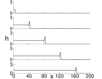
Figure 1: The flow down an inverted substrate ($D=-1.0$). From top to bottom, $t=0$, $40$, $80$, $120$, $160$.

Type 2: $-1.9\leq D<-1.1$. The capillary ridge is still observed; however, here it is followed by a wave train. Figure 2 shows as an example of the evolution for $D=-1.5$. Waves keep forming behind the front, and, furthermore, they move faster than the front itself. Therefore the first wave behind the front catches up with the ridge, interacts and merges with it. The other important feature of the results is that there are three different states observed behind the capillary ridge: two types of waves and a constant state. These states can be clearly seen in the last frame of Fig. 2. Immediately behind the front, there is a range characterized by waves resembling solitary ones [10] discussed in some more detail below. This range is followed by another one with sinusoidal shape waves. Finally there is a constant state behind. Such mixed-wave feature remains present even for very long time. To illustrate this, Fig. 3 shows the result at much later time, $t=340$, using an increased domain size.

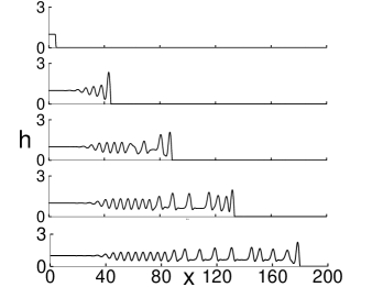
Figure 2: The flow down an inverted substrate ($D=-1.5$). From top to bottom, $t=0$, $40$, $80$, $120$, $160$ (enhanced online).

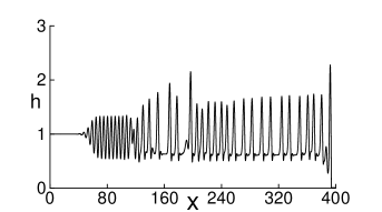
Figure 3: The flow down an inverted substrate ($D=-1.5$) at $t=340$.

Also, Fig. 4, which includes typical results from the Type 3 regime discussed below, imply that Type 2 corresponds to a transitional regime between the Types 1 and 3. Additional simulations (not shown here) suggest that the regions where the waves are present within Type 2 regime become more and more extended as the magnitude of $D$ is increased. Future insight regarding the nature of wave formation in Type 2 regime is discussed in the following Section. Here we note that the available animations of wave evolution are very helpful to illustrate the complexity of wave interaction in Type 2 and Type 3 regime discussed next.

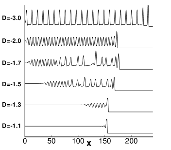
Figure 4: Comparison of the results for different $D$’s at $t=150$.

Type 3: $-3.0\leq D<-1.9$. This is a nonlinear steady traveling wave regime. There is no damping of surface oscillations that we observed e.g., in Fig. 2. Figure 5 shows an example obtained using $D=-2.0$. Here, a wave train forms behind the first (still dominant) capillary ridge. Similarly as before, since this wave train travels faster than the fluid front, there is an interaction between the first of these waves and the capillary ridge. On the other end of the domain, these waves also interact with the inlet at $x=0$; the role of this interaction is discussed in more details later in Sec. 4.3.

We find that the Type 3 includes two sub-types. For smaller absolute values of $D$, such as $D=-2.0$, one finds sinusoidal waves as shown in Fig. 5. For larger magnitudes of $D$, we find solitary type waves, the structures sometimes referred to as ‘solitary humps’, such that characteristic dimension of a hump is much smaller than the distance between them [10]. Both types of waves are illustrated in Fig. 4, which shows the results for $D=-2.0$ and $D=-3.0$, and in Fig. 6, showing the typical wave profiles for $D=-2.0$, $D=-2.5$ and $D=-3.0$. The wave profiles that we find are very similar to the ones observed for continuous films exposed to periodic forcing [9, 22, 21]. For the flow considered here, the governing parameter is $D$, in contrast to the forcing frequency in the works referenced above.

In the next section, we will discuss in more detail some features of the results presented here. Here, we only note that it may be surprising that all the waves discussed are found using numerical simulations, remembering that we do not impose forcing on the inlet region, and furthermore, we do not include inertial effects in our formulation. Instead, we have a hanging film with a contact line in the front. Therefore, it appears that the presence of fronts and corresponding contact lines plays an important role in instability development.

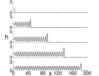
Figure 5: The flow down an inverted substrate ($D=-2.0$). From top to bottom, $t=0$, $40$, $80$, $120$, $160$. Note that there is a continuous interaction of the surface waves and the front, since the surface waves travel faster than the front itself (enhanced online).

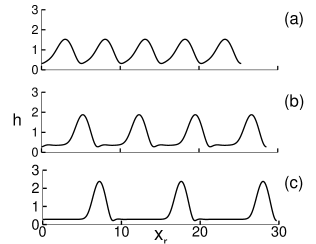
Figure 6: Wave profile for different $D$’s. (a): $D=-2.0$; (b): $D=-2.5$; (c): $D=-3.0$. The wave profile have been shifted to illustrate the difference in wave number, i.e., $x_{r}=x-x_{0}$ where $x_{0}$ is an arbitrary shift.

We note that it is possible in principle to carry out the computations also for more negative $D$’s. We find that, as absolute value of $D$ is increased, the amplitude of the waves, including the capillary ridge, increases, and furthermore, the periodicity of the wave train following the capillary ridge is lost. However, since the observed structures are characterized by relatively large spatial gradients which at least locally are not consistent with the lubrication approximation, we do not show them here. It would be of interest to consider this flow configuration outside of lubrication approximation and analyze in more detail the waves in this regime. In addition, this regime should also include the transition from flow to detachment, the configuration related to the so call ‘tea-pot’ effect [27, 28, 29].

4 Discussion of the results

In this Section, we discuss in some more detail the main features of the numerical results and compare them to the ones that can be found in the literature. We consider in particular the difference between various regimes discussed above. In Sec. 4.1 we give the main results for the velocities of the film front and the propagating waves. In Sec. 4.2 we discuss the main features of the instability that forms and show that the presence of contact line is important in determining the properties of the waves, including their typical wavelength. Then we finally discuss one question that was not considered explicitly so far: What is the source of instability? As we already suggested, contact line appears to play a role here. However, it is appropriate to also discuss the influence of numerical noise on instability development, shown in Sec. 4.3. As we will see, both aspects are important to gain better understanding of the problem.

4.1 Front speed and wave speed

Figure 7 compares the velocity of the leading capillary ridge for different $D$’s. The speed of the traveling wave solution, $U$, is $1+b+b^{2}$, and is exactly the front speed for $D=-1.0$, as discussed in Appendix A.1 in connection to Fig. 12. For all other cases shown, the velocity of the leading capillary ridge oscillates around $U$, due to the interaction between the leading capillary ridge and the upcoming waves.

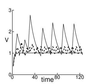
Figure 7: Velocity profile of the leading capillary ridge for different $D$’s. $D=-1.0$ (solid), $D=-2.0$ (dashed), $D=-3.0$ (dotted).

Table 1 shows the speed of waves in Type 3 regime. As we can see, the wave speed in all cases is greater than $U$. A simple explanation on why the waves move faster than the fluid front itself is that the motion of the front is resisted by the precursor film (recall that in the limit $b\rightarrow 0$, there is infinite resistance to the fluid motion within the formalism implemented here). The surface waves however, travel with a different, larger speed. Therefore, the upcoming waves eventually catch up with the front, interact, and merge into a new capillary ridge. Figure 8 illustrates this process. Due to the conservation of mass, the height of the leading capillary ridge increases strongly right after the merge. Also the speed of the capillary ridge increases. As the leading capillary ridge moves forward, its height decreases until next wave arrives. That is the reason why we see such pulse-like velocity profiles in Fig. 7; each pulse is a sign of a wave reaching the front. In the Type 2 regime, the velocity of the front shows similar oscillatory behavior, although the approximate periodicity of the oscillations is lost due to more irregular structure of the surface waves. Going back to the Type 3 and Table 1, we see that wave amplitude and speed are both increasing with $D$, consistently with the behavior of continuous vertically falling films [19, 22].

$D$	wave amplitude	wave speed
-2.0	1.53	1.88
-2.5	1.88	2.20
-3.0	2.38	2.65

Table 1: Wave amplitude and wave speed for different $D$’s in Type 3 regime. Note that the wave speed is always larger than the capillary ridge speed, shown in Fig. 7.

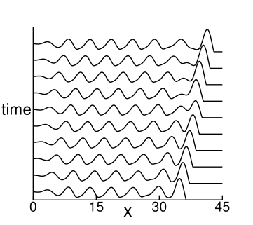
Figure 8: Wave interaction with the capillary ridge. Time evolution is from the bottom to the top, $D=-2.0$.

4.2 Absolute versus convective instability

Here we analyze some features of the results in particular from Type 1 and Type 2 regimes using linear stability analysis. Let us ignore for a moment the contact line, and analyze stability of a flat film. The basic framework is given in the Appendix A2. We realize that Eq. (16) can be reduced to a linear Kuramoto-Sivashinsky equation in the reference frame moving with the nondimensional speed equal to $3$. Consider then the evolution of a localized disturbance imposed on the flat film at $t=0$. This disturbance will transform into an expanding wave packet with two boundaries moving with the velocities $(x/t)_{-}$ and $(x/t)_{+}$ [35]. In the laboratory frame, these velocities are given by [36]

$${\left(x\over t\right)}_{\pm}\approx 3\pm 1.62(-D)^{3/2}~{}.$$ (6)

The right going boundary moves faster than the capillary ridge and can be ignored. Considering now the left boundary, we see that there is a range $D_{c1}>D>D_{c2}$ such that the speed of this boundary is positive and smaller than $U$. Alternatively, one can use the approach from [37], which is based on studying the behavior of the curve $\omega_{i}=0$ in the complex $k$ plane, with the same result. Using either approach, one finds $D_{c1}\approx-1.15$ and $D_{c2}\approx-1.51$. This result explains the boundary between the Type 1 and Type 2 regimes since for Type 1, $D>D_{c1}$ and the left boundary moves faster than the front itself. For $D>D_{c2}$, the speed of the left boundary is positive, and therefore the instability is of convective type. This can be seen from Fig. 4 and is illustrated in detail in Table 2. In this table, we show the value of $D_{lin}$, predicted by Eq. (6), using the position of the left boundary $x_{-}$ obtained numerically. While the agreement between $D_{num}$ and $D_{lin}$ is generally very good, we notice some discrepancy for $D_{num}=-1.7$; this can be explained by the fact that for this $D_{num}$ there is already some interaction with the boundary at $x=0$.

These results suggests that we should split our Type 2 regime into two parts: Type 2a, for which the speed of the left boundary is positive ($D>D_{c2}$), and Type 2b, for which the speed of the boundary is negative and the instability is of absolute type. In Type 2a regime, a flat film always exists and expands to the right with time. In Type 2b regime, flat film disappears after sufficiently long time. As an illustration, we note that $D=-1.5$ shown in Fig. 2, lies approximately at the boundary of these two regimes, since here the length of the flat film is almost time-independent. We also note that in Type 2b regime, we always observe two types of waves, in contrast to Type 3; that is, the structure shown e.g. in Fig. 4 for $D=-1.7$ persists for a long time.

$D_{num}$	$x_{-}$	$(x/t)_{-}$	$D_{lin}$
-1.1	150	1.00	-1.15
-1.3	100	0.66	-1.28
-1.5	30	0.20	-1.44
-1.7	0	0.00	-1.51

Table 2: $D_{num}$ is the value of $D$ used in simulations, the position $x_{-}$ is taken from Fig. 4 ($t=150$) and used to calculate the speed $(x/t)_{-}$; $D_{lin}$ is calculated from Eq. (6) using the negative sign.

To allow for better understanding of the properties of the waves that form, in the results that follow we have modified our initial condition (put $x_{f}=50$) to allow for longer wave evolution without interaction of the wave structure with the domain boundary ($x=0$). Figure 9 shows that for $D=-2.0$, the waves form immediately behind the leading capillary ridge; see also the animation attached to this figure. For longer time ($t>40$ in Fig. 9), the disturbed region covers the whole domain as expected based on the material discussed in Sec. 4.2. Note that even for $t=100$ we still see transient behavior: the long time solution for this $D$ consists of uniform stream of waves and is shown in Fig. 6(a). This long time solution is independent of the initial condition. However, the time period needed for this uniform stream of waves to be reached depends on the initial film length and is much longer for larger $x_{f}$ used here.

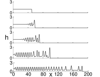
Figure 9: $D=-2.0$. From top to bottom, $t=0$, $10$, $20$, $40$, $100$. For early times, the contact line induced instability propagates to the left. For longer times, sine-like and solitary-like waves are observed, covering the whole domain by $t=40$ (enhanced online).

Figure 9 suggests that contact line plays a role in wave formation (the other candidate, numerical noise, is discussed below). One may think of contact line as a local disturbance. It generates an expanding wave packet as we have just shown, and the velocities of the two boundaries are given by Eq. (6). In particular, for $D<D_{c1}$, the left boundary moves slower than the capillary ridge. The wave number, $k_{l}$, along this boundary is defined by

$$\left.\left(\frac{\partial\omega}{\partial k}\right)\right|_{k=k_{l}}=\left(\frac{x}{t}\right)_{-},$$ (7)

and it should be compared to the sine-like waves that form due to contact line presence (such as the waves shown in Fig. 9 for early times). Table 3 gives this comparison: the values of $k_{l}$ for a given $D$ are shown in the second column, followed by the numerical results for the wave number, $q_{n}$. We find close agreement, suggesting that $k_{l}$ captures very well the basic features of the waves that form due to contact line presence. Furthermore, both $q_{n}$ and $k_{l}$ are much larger than $k_{m}$, the most unstable wave number expected from the linear stability analysis (LSA) described below (vis. the last column in Table 3). This difference allows to clearly distinguish between the contact line induced waves and the noise induces ones, discussed in what follows.

$D$	$k_{l}$	$q_{n}$	$k_{m}$
-1.3	1.10	1.10	0.81
-1.5	1.18	1.14	0.87
-1.7	1.25	1.23	0.92
-2.0	1.36	1.35	1.00
-2.5	1.52	1.48	1.12

Table 3: The second column shows theoretical results for the wave number of the left moving boundary ($k_{l}$), in the limit of small oscillations, see Eq. (7). The third column shows the wave number resulting from simulations for different $D$’s in Type 2 and Type 3 regimes in the contact line induced part (e.g., the waves shown in Fig. 2 ($t=160$) for $40<x<80$ for Type 2, or in Fig. 9 ($t=20$) about $x=40$). The last column shows the wave number of maximum growth, $k_{m}$, resulting from the linear stability analysis.

4.3 Noise induced waves

The results of LSA of a flat film (see Sec. A.2) for the most unstable wave number shown in Table 3, confirm that a flat film is unstable to long wave perturbations for negative $D$’s. Although our base state is not a flat film, there is clearly a possibility that numerical noise, which includes long wave component, could grow in time and influence the results. As an example, we consider again $D=-2.0$. Similar results and conclusions can be reached for other values of $D$.

Let us first discuss expected influence of numerical noise. For $D=-2.0$, the LSA shows that it takes $30$ time units for the noise of initial amplitude of $10^{-16}$ (typical for double precision computer arithmetic) to grow to $10^{-2}$. LSA also shows that waves with small amplitude should move with the speed $3$. That is, natural noise, which is initially at $x=0$, should arrive to $x=90$ after $30$ time units. Figure 10 illustrate this phenomenon. As $t$ approaches $30$, we see that the noise appears at about $x=90$. Noise manifests itself through the formation of waves behind the contact line induced waves which were already present for earlier times; see also the animation attached to Fig. 10. To further confirm that this new type of waves is indeed due to numerical noise, we have also performed simulations using quadruple precision computer arithmetic. Figure 11 shows the outcome: with higher precision, the noise induced waves are absent, as expected. We note that in order to be able to clearly identify various regimes, we take $x_{f}=150$ in Figs. 10 and 11, so that no influence of the boundary condition at $x=0$ is expected.

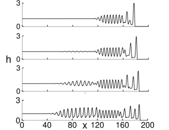
Figure 10: $D=-2.0$. From top to bottom, $t=25$, $27$, $29$, $31$ (double precision). The initial condition for this simulation is chosen to be a hyperbolic tangent with contact line located at $x=150$. Also note the comparison between contact line induced wave ($120<x<190$) and error-induced wave ($50<x<120$) (enhanced online).

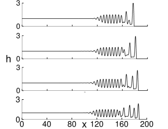
Figure 11: $D=-2.0$. From top to bottom, $t=25$, $27$, $29$, $31$ (quadruple precision). The initial condition is the same as in Fig. 10.

In Fig. 10 ($t=31$), we can clearly distinguish between the waves induced by contact line $(120<x<190)$, and the ‘natural waves’ induced by noise $(50<x<120)$. The main difference is the wavelength. The contact line induced waves have its specific wavelength, $2\pi/k_{l}$, while the noise induced ones are characterized by a wavelength, $\lambda$, corresponding very closely to the mode of maximum growth, $\lambda\approx{2\pi/k_{m}}$, obtained using LSA. This can be clearly seen by comparing the numerical results shown in Fig. 10 ($t=31$) with the LSA results given in Table 3.

To summarize, the evolution of the wave structure in the Type 2 and Type 3 regimes proceeds as follows. First one sees formation of contact line induced waves, characterized by relatively short wavelengths (compared to what would be expected based on the LSA of a flat film). Depending on the value of $D$, one may also see formation of solitary-looking waves immediately following the capillary ridge. At some later time, these waves are followed by noise-induced one. These three types of waves are all presented in Fig. 10. Then, at even later times, when the waves cover the whole domain and interact with the $x=0$ boundary, the final wave pattern forms, as illustrated for $D=-2.0$ by Fig. 4. In Conclusions we discuss briefly under which conditions these waves may be expected to be seen in physical experiments.

Remark I. Finally, one may wonder why the traveling wave solution for $D=-1.0$ shown in Fig. 1 remains stable for such a long time. Recall that the LSA predicts that natural noise with amplitude $10^{-16}$ should grow to $10^{-2}$ in $130$ time units, while our numerical result shows that flat film is preserved even for $t=160$. The reason is the domain size. It takes approximately $66$ time units for noise to travel across the domain (moving with the speed equal to 3), and the noise can only grow from $10^{-16}$ to $10^{-9}$ during this time period for $D=-1$. This is why we do not see the effect of noise for small $D$’s.

Remark II We have used LSA of a flat film (therefore, ignoring contact line presence) to predict the evolution of the size of the region covered by waves in Sec. 4.2. However, in order to understand the properties of the waves that form in this region, one has to account for the presence of a front, as discussed in Sec. 4.3. In our simulations, we are able to tune the influence of noise on the results (vis. Fig. 10 versus Fig. 11). In physical experiments, these two effects will quite possibly appear together.

4.4 Relation of physical quantities with non-dimensional parameter $D$

It is useful to discuss the relation between the nondimensional parameter $D$ in our model, Eq. (2), and physical quantities. In particular, we recall that there are two quantities, $h_{0}$ (film thickness) and $\alpha$ (inclination angle) which can be adjusted in an experiment, and here we discuss how variation of each of these modifies our governing parameter and the results. We also relate $D$ to the fluid flux and the Reynolds number.

The velocity scaling in Eq. (2) can be expressed as

$$U=\frac{\rho g}{3\mu}h^{2}_{0}\sin\alpha.$$

Therefore the parameter $D$ can be written as

$$D=\left(\frac{\rho g}{\gamma}\right)^{1/3}h^{2/3}_{0}\frac{\cos\alpha}{(\sin\alpha)^{2/3}}.$$ (8)

In our simulations, the flux $Q$ in the $x$-direction is been kept constant and equals to $1$. The dimensional flux is

$$Q=1\cdot h_{0}\cdot U=\frac{\rho g}{3\mu}h^{3}_{0}\sin\alpha.$$ (9)

Reynolds number can be expressed as

$$Re=\frac{\rho U\ell}{\mu}=\frac{(\rho^{5}g^{2}\gamma^{2})^{1/3}}{3\mu^{2}}h_{0}^{7/3}(\sin\alpha)^{2/3}.$$ (10)

We note that there is no contradiction in considering $Re$, although inertial effects were neglected in deriving the formulation that we use. The present formulation is valid for $Re=O({1/\epsilon})$ or smaller, where $\epsilon\ll 1$ is the ratio of the length scales in the out-of-plane and in-plane directions [38]. Considering the influence of $Re$ for this range is permissible.

	$\alpha$ fixed				$h_{0}$ fixed
	$D>0$	$D<0$			$D>0$	$D<0$
$|D|$	$\uparrow$	$\uparrow$		$|D|$	$\uparrow$	$\uparrow$
$h_{0}$	$\uparrow$	$\uparrow$		$\alpha$	$\downarrow$	$\uparrow$
$Q$	$\uparrow$	$\uparrow$		$Q$	$\downarrow$	$\downarrow$
$Re$	$\uparrow$	$\uparrow$		$Re$	$\downarrow$	$\downarrow$
$U$	$\uparrow$	$\uparrow$		$U$	$\downarrow$	$\downarrow$

Table 4: Relation of the parameter $D$ to other parameters for fixed contact angle, $\alpha$ (left), and for fixed film thickness, $h_{0}$ (right). The up arrow $\uparrow$ means an increase and down arrow $\downarrow$ means a decrease.

The relation between $D$ and relevant physical quantities is shown in Table 4. For fixed inclination angle an increase of the magnitude of $D$ is equivalent to an increase of the film thickness, flux and Reynolds number. On the other hand, for fixed film thickness, i.e., $h_{0}=$constant, raising the magnitude of $D$ leads to lower flux and Reynolds number, and the inclination angle approaches horizontal. We can use this connection to relate to the experimental results of Alekseenko et al. (see Fig. 11 in [39]). They performed the experiments with fixed inclination angle and increasing the flux, which corresponds to an increase of the magnitude of $D$ in our case. Our Fig. 6 shows that the trend of our results is the same as in the above experiments. In addition, the results in [29] suggest that further increasing of the flux leads to pinch-off, consistently with our results, since for $D<-3.0$, numerics suggest that lubrication assumption is not valid.

Finally, one should recall that lubrication approximation is derived under the condition of small slopes, which translates to

$$\left(\frac{h_{0}\sqrt{\sin\alpha}}{a}\right)^{2/3}\ll 1,$$ (11)

if nondimensional slopes are O$(1)$, see e.g. [31]; here $a=\sqrt{\gamma/\rho g}$ is the capillary length. In addition, by combining the above lubrication limit with Eq. (8), one gets the following condition (see also [40]):

$$|D|<|\cot\alpha|.$$ (12)

Therefore, for a given $D$, there exists a range of inclination angle for which the thin film model, Eq. (2), is valid. Table 5 shows this range for some values of $D$.

$D$	$\alpha_{c}$
-1.0	$135^{o}$
-1.5	$147^{o}$
-2.0	$154^{o}$
-3.0	$162^{o}$

Table 5: $\alpha_{c}$ is the inclination angle at which lubrication theory ceases to be formally valid.

5 Conclusions

In this paper we report numerical simulation of thin film equation (2) on inverted substrate. It is found that by changing a single parameter $D$, one can find three different regimes of instability. Each regime is characterized by different type of waves. Some of these waves show similar properties as the ones observed in thin liquid films with periodic forcing. However, in contrast to those waves produced by perturbations at the inlet region, our instability comes from the front. We find that the presence of a contact line leads to free surface instability without any additional perturbation. According to linear stability analysis, we know that for negative $D$, the model problem, Eq. (2), is unstable in the sense that any numerical disturbance grows exponentially in time. However, we can also take advantage of the stability analysis to separate the instability caused by noise and any other sources.

Finally, we may ask about experimental conditions for which the waves discussed here can be observed. As an example, consider polydimethylsiloxane (PDMS), also known as silicon oil (surface tension: $21dyn/cm$; density: $0.96g/cm^{3}$), and discuss the experimental parameters for which the condition $|D|<3.0$ is satisfied. For $\alpha=170^{o}$ (the value used in [39]), the thickness should be less than $1.4mm$. Table 6 gives the values for this, as well as for some other $D$’s. However, one should recall that Eq. (12) shows that our model is formally valid only up to a certain $D$ for a given inclination angle $\alpha$. In addition, one should be aware that the use of lubrication approximation is easier to justify for inclination angles further away from the vertical.

$\alpha$	$D$	$h_{0}$($mm$)
$150^{o}$	-1.0	0.93
	-1.5	1.7
$170^{o}$	-1.0	0.27
	-2.0	0.75
	-3.0	1.40

Table 6: $h_{0}$ is the film thickness defined by Eq. (8).

Acknowledgments. The authors thank Linda J. Cummings and Burt Tilley for useful comments. They also acknowledge very useful input from anonymous referee leading to the material presented in Sec. 4.2. This work was partially supported by NSF grant No. DMS-0908158.

Appendix A Evolution of small perturbations

Equation (3) is a strongly nonlinear PDE and, to our knowledge, has no analytical solutions. In this appendix, we present two analytical approaches which consider evolution of small perturbations from a base state within linear approximation. While these results are useful for the purpose of verifying numerical results, they also provide a very useful insight into formation and evolution of various instabilities discussed in this work.

A.1 Traveling wave solution

Setting $s=x-Ut$ in Eq. (3), a traveling wave $H(s)=h(x,t)$ must satisfy

$$-UH+[H^{3}(H^{\prime\prime\prime}-DH^{\prime}+1)]=c.$$ (13)

Imposing the conditions $H\rightarrow 1$ as $s\rightarrow-\infty$, and $H\rightarrow b$ as $s\rightarrow\infty$, we find $U=1+b+b^{2}$, $c=-b-b^{2}$ [41, 5]. The traveling wave speed, $U$, is useful for verifying whether or not the numerical result is a traveling wave solution.

Figure 12 shows a typical profile of the traveling wave solution for $D=-1$. A capillary ridge forms behind the fluid front, similarly as for the flow down a vertical or inclined ($D>0$) substrate. We also find that there exists a long oscillatory region behind the capillary ridge. To analyze this ’tail’, we expand Eq. (13) around the base state, $H\equiv 1$, and consider the evolution of a small perturbation of the form $exp(qs)$, where $q=q_{r}+iq_{i}$. We find

$$-8q_{r}^{3}+2Dq_{r}+2-b-b^{2} = 0,$$ (14)

$$q_{i}^{2}+D = 3q_{r}^{2}.$$ (15)

Table 7 shows the only positive root for $q_{r}$, for a set of D’s. The positivity of this root signifies that the amplitude of the tail decays exponentially in the $-x$ direction, as also suggested by the insets of Figure 12. Furthermore, as shown in Table 7, $q_{r}$ decreases for more negative $D$’s, meaning that the tail is longer for these $D$’s. This table also shows the imaginary part of $q$; we see an increase of its magnitude as $D$ becomes more negative, suggesting shorter and shorter wavelengths in the tail.

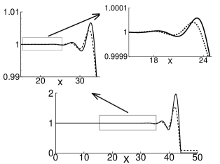
Figure 12: Traveling wave solution of $D=-1$ case at three different scales with precursor thickness $b=0.01$ (solid) and $b=0.1$ (dashed). Note that the precursor thickness only changes amplitude of the traveling wave profile but not the wavelength. The arrows point to the zoomed-in regions.

Tail behavior is very useful for computational reasons. For example, to solve Eq. (13) by shooting method, one can evaluate suitable shooting parameters through Eqs. (14,15).

$D$	$q_{r}$	$q_{i}$
0	0.63	1.09
-1.0	0.50	1.32
-2.0	0.38	1.56
-3.0	0.30	1.81

Table 7: Properties of the damped oscillatory region (tail) behind the capillary ridge.

Figure 12 also shows the effect of precursor thickness on traveling wave solution. It is found that while the precursor thickness changes the height of the capillary ridge, it has almost no effect on the wavelength of the tail.

A.2 Linear stability analysis

Another approach to analyze the stability of a flat film, is classical linear stability analysis. Assume $h=1+\xi$ where $\xi\ll 1$. Eq. (3) can be simplified to the leading order as

$$\xi_{t}+\xi_{xxxx}-D\xi_{xx}+3\xi_{x}=0.$$ (16)

By putting $\xi\sim\exp i(kx-\omega t)$, where $\omega=\omega_{r}+i\omega_{i}$, we obtain the dispersion relation

$$-i(\omega_{r}+i\omega_{i})+k^{4}+Dk^{2}+3ik=0,$$ (17)

hence

$$\omega_{r}=3k,\quad\omega_{i}=-(k^{4}+Dk^{2})=-(k^{2}+D/2)^{2}+D^{2}/4.$$ (18)

As a result, for non-negative $D$’s, a flat film is stable under small perturbations. For negative $D$’s, it is unstable for the perturbations characterized by sufficiently large wavelengths. The critical wave number $k_{c}=\sqrt{-D}$, and the perturbation with wave number $k_{m}=\sqrt{-D/2}$ has the largest growth rate. Besides, the speed of a linear wave is $3$, and it is significantly larger than the traveling wave speed, $U$. As discussed in the main body of the text, this speed is very important to identify the waves induced by natural noise.

In addition, one should note that the maximum growth rate increases as inclination angle $\alpha$ goes from $\pi/2$ to $\pi$. Particularly, in the limiting case $\alpha\rightarrow\pi$ (hanging film), the growth rate is exactly the same as for thin film Rayleigh-Taylor instability (e.g., [42]). Note that the scaling used in present work is not appropriate for $\alpha\rightarrow\pi$; to establish the result for this case, one should consider a different scaling, or the dimensional formulation of the problem.

References

- [1] H. Huppert. Flow and instability of a viscous current down a slope. Nature, 300:427, 1982.
- [2] N. Silvi and E. B. Dussan V. On the rewetting of an inclined solid surface by a liquid. Phys. Fluids, 28:5, 1985.
- [3] A. M. Cazabat, F. Heslot, S. M. Troian, and P. Carles. Fingering instability of thin spreading films driven by temperature gradients. Nature, 346:824, 1990.
- [4] J. R. de Bruyn. Growth of fingers at a driven three–phase contact line. Phys. Rev. A, 46:4500, 1992.
- [5] A. L. Bertozzi and M. P. Brenner. Linear stability and transient growth in driven contact lines. Phys. Fluids, 9:530, 1997.
- [6] P. L. Kapitsa and S. P. Kapitsa. Wave flow of thin fluid layers of liquid. Zh. Eksp. Teor. Fiz., 19:105, 1949.
- [7] J. Liu and J. P. Gollub. Onset of spatially chaotic waves on flowing films. Phys. Rev. Lett., 70:2289, 1993.
- [8] J. Liu, J. D. Paul, and J. P. Gollub. Measurement of the primary instabilities of film flows. J. Fluid Mech., 250:69, 1993.
- [9] J. Liu and J. P. Gollub. Solitary wave dynamics of film flows. Phys. Fluids, 6:1702, 1994.
- [10] H.-C. Chang and E. A. Demekhin. Complex wave dynamics on thin films. Elsevier, New York, 2002.
- [11] S. V. Alekseenko, V. E. Nakoryakov, and B. G. Pokusaev. Wave flow of liquid films. Begell House, New York, 1994.
- [12] T. B. Benjamin. Wave formation in laminar flow down an inclined plane. J. Fluid Mech., 2:554, 1957.
- [13] C. S. Yih. Stability of liquid flow down an inclined plane. Phys. Fluids, 6:321, 1963.
- [14] H.-C. Chang. Wave evolution on a falling film. Annu. Rev. Fluid Mech., 26:103, 1994.
- [15] S. Saprykin, E. A. Demekhin, and S. Kalliadasis. Two-dimensional wave dynamics in thin films. I. Stationary solitary pulses. Phys. Fluids, 17:117105, 2005.
- [16] A. Oron, S. H. Davis, and S. G. Bankoff. Long-scale evolution of thin liquid films. Rev. Mod. Phys., 69:931, 1997.
- [17] Y. Y. Trifonov and O. Y. Tsvelodub. Nonlinear waves on the surface of a falling liquid film. part 1. waves of the first family and their stability. J. Fluid Mech., 229:531, 1991.
- [18] H.-C. Chang, E. A. Demekhin, and S. S. Saprikin. Noise-driven wave transitions on a vertically falling film. J. Fluid Mech., 462:255, 2002.
- [19] S. V. Alekseenko, V. E. Nakoryakov, and B. G. Pokusaev. Wave formation on a vertically falling liquid film. AIChE J., 31:1446, 1985.
- [20] N. A. Malamataris, M. Vlachogiannis, and V. Bontozoglou. Solitary waves on inclined films: flow structure and binary interactions. Phys. Fluids, 14:1082, 2002.
- [21] T. Nosoko and A. Miyara. The evolution and subsequent dynamics of waves on a vertically falling liquid film. Phys. Fluids, 16:1118, 2004.
- [22] H.-C. Chang, E. A. Demekhin, and D. I. Kopelevich. Nonlinear evolution of waves on a vertically falling film. J. Fluid Mech., 250:433, 1993.
- [23] H. S. Kheshgi and L. E. Scriven. Disturbed film flow on a vertical plate. Phys. Fluids, 30:990, 1987.
- [24] R. R. Mudunuri and V. Balakotaiah. Solitary waves on thin falling films in the very low forcing frequency limit. AIChE J., 52:3995, 2006.
- [25] J. Tihon, K. Serifi, K. Argyriadi, and V. Bontozoglou. Solitary waves on inclined films: their characteristics and the effects on wall shear stress. Exp. Fluids, 41:79, 2006.
- [26] V. Shikin and E. Lebedeva. Anti-gravitational instability of the neutral helium film. J. Low Temp. Phys., 119:469, 2000.
- [27] W. G. Pritchard. Instability and chaotic behaviour in a free-surface flow. J. Fluid Mech., 165:1, 1986.
- [28] S. F. Kistler and L. E. Scriven. The teapot effect: sheet-forming flows with deflection, wetting and hysteresis. J. Fluid Mech., 263:19, 1994.
- [29] A. Indeikina, I. Veretennikov, and H.-C. Chang. Drop fall-off from pendent rivulets. J. Fluid Mech., 338:173, 1997.
- [30] J. A. Diez, L. Kondic, and A. L. Bertozzi. Global models for moving contact lines. Phys. Rev. E, 63:011208, 2001.
- [31] L. Kondic. Instabilities in gravity driven flow of thin liquid films. SIAM Review, 45:95, 2003.
- [32] L. W. Schwartz. Viscous flows down an inclined plane: instability and finger formation. Phys. Fluids A, 1:443, 1989.
- [33] A. Oron and P. Rosenau. Formation of patterns induced by thermocapillarity and gravity. J. Phys. (France), 2:131, 1992.
- [34] L. Kondic and J. A. Diez. Flow of thin films on patterned surfaces: Controlling the instability. Phys. Rev. E, 65:045301, 2002.
- [35] P. Huerre and P. A. Monkewitz. Local and global instabilities in spatially developing flows. Annu. Rev. Fluid Mech., 22:473, 1990.
- [36] H.-C. Chang, E. A. Demekhin, and D. I. Kopelevich. Stability of a solitary pulse against wave packet disturbances in an active medium. Phys. Rev. Lett., 75:1747, 1995.
- [37] A. S. Fokas and D. T. Papageorgiou. Absolute and convective instability for evolution PDEs on the half-line. Stud. Appl. Math., 114:95, 2005.
- [38] D. J. Acheson. Elementary Fluid Dynamics. Clarendon Press, Oxford, 1990.
- [39] S. V. Alekseenko, D. M. Markovich, and S. I. Shtork. Wave flow of rivulets on the outer surface of an inclined cylinder. Phys. Fluids, 8:3288, 1996.
- [40] R. Goodwin and G. M. Homsy. Viscous flow down a slope in the vicinity of a contact line. Phys. Fluids A., 3:515, 1991.
- [41] S. M. Troian, E. Herbolzheimer, S. A. Safran, and J. F. Joanny. Fingering instabilities of driven spreading films. Europhys. Lett., 10:25, 1989.
- [42] J. M. Burgess, A. Juel, W. D. McCormick, J. B. Swift, and H. L. Swinney. Suppression of dripping from a ceiling. Phys. Rev. Lett., 86:1203, 2001.