Discussion of: Brownian distance covariance

10.1214/09-AOAS312

Discussion on Brownian distance covariance by G. J. Szekely and M. L. Rizzo

and r1Supported in part by NSF Grant DMS-09-06808.

Szekely and Rizzo present a new interesting measure of correlation. The idea of using $\int|\phi_{n}(u,v)-\phi_{n}^{(1)}(u)\phi_{n}^{(2)}(v)|^{2}\,d\mu(u,v)$, where $\phi_{n}$, $\phi_{n}^{(1)}$, $\phi_{n}^{(2)}$ are the empirical characteristic functions of a sample $(X_{i},Y_{i})$, $i=1,\ldots,n$, of independent copies of $X$ and $Y$ is not so novel. A. Feuerverger considered such measures in a series of papers 4 . Aiyou Chen and I have actually analyzed such a measure for estimation in 3 in connection with ICA.

However, the choice of $\mu(\cdot,\cdot)$ which makes the measure scale free, the extension to $X\in\mathbb{R}^{p},Y\in\mathbb{R}^{q}$ and its identification with the Brownian distance covariance is new, surprising and interesting.

There are three other measures available, for general $p$, $q$:

1. The canonical correlation $\rho$ between $X$ and $Y$.

2. The rank correlation $r$ (for $p=q=1$) and its canonical correlation generalization.

3. The Renyi correlation $R$.

All vanish along with the Brownian distance (BD) correlation in the case of independence and all are scale free. The Brownian distance and Renyi covariance are the only ones which vanish iff $X$ and $Y$ are independent.

However, the three classical measures also give a characterization of total dependence. If $|\rho|=1$, $X$ and $Y$ must be linearly related; if $|r|=1$, $Y$ must be a monotone function of $X$ and if $R=1$, then either there exist nontrivial functions $f$ and $g$ such that $\mathbb{P}(f(X)=g(Y))=1$ or at least there is a sequence of such nontrivial functions $f_{n}$, $g_{n}$ of variance $1$ such that $\mathbb{E}(f_{n}(X)-g_{n}(Y))^{2}\rightarrow 0$.

In this respect, by Theorem 4 of Szekely and Rizzo, for the common $p=q=1$ case, BD correlation does not differ from Pearson correlation.

Although we found the examples varied and interesting and the computation of $p$ values for the BD covariance effective, we are not convinced that the comparison with the rank and Pearson correlations is quite fair, and think a comparison to $R$ is illuminating.

Intuitively, the closer the form of observed dependence is to that exhibited for the extremal value of the statistic, the more power one should expect. Example 1 has $Y$ as a distinctly nonmonotone function of $X$ plus noise, a situation where we would expect the rank correlation to be weak and, similarly, the other examples correspond to nonlinear relationships between $X$ and $Y$ in which we would expect the Pearson correlation to perform badly. In general, for goodness of fit, it is important to have statistics with power in directions which are plausible departures; see Bickel, Ritov and Stoker 1 .

Ying Xu is studying, in the context of high dimensional data, a version of empirical Renyi correlation different from that of Breiman and Friedman 2 .

Let $f_{1},f_{2},\ldots$ be an orthonormal basis of $L_{2}(P_{X})$ and $g_{1},g_{2},\ldots$ an orthonormal basis of $L_{2}(P_{Y})$, where $L_{2}(P_{X})$ is the Hilbert space of function $f$ such that $\mathbb{E}f^{2}(X)<\infty$ and similarly for $L_{2}(P_{Y})$.

Let the $(K,L)$ approximate Renyi correlation be defined as

$$\max\Biggl{\{}\mbox{corr}\Biggl{(}\sum_{k=1}^{K}\alpha_{k}f_{k}(X),\sum_{l=1}^{L}\beta_{l}g_{l}(Y)\Biggr{)}\Biggr{\}},$$

where corr is Pearson correlation.

This is seen to be the canonical correlation of $\underline{f}(X)$ and $\underline{g}(Y)$, where $\underline{f}\equiv(f_{1},\ldots,f_{K})^{T}$, $\underline{g}\equiv(g_{1},\ldots,g_{L})^{T}$, and is easily calculated as a generalized eigenvalue problem. The empirical $(K,L)$ correlation is just the solution of the corresponding empirical problem where the variance covariance matrices $\operatorname{Var}\underline{f}(X)\equiv\mathbb{E}[\underline{f_{c}}(X)\underline{f_{c}}^{T}(X)]$ where $\underline{f_{c}}(X)\equiv\underline{f}(X)-\mathbb{E}\underline{f}(X)$, $\operatorname{Var}\underline{g}(Y)$ and $\operatorname{Cov}(\underline{f}(X),\underline{g}(Y))$ are replaced by their empirical counterparts. For $K,L\rightarrow\infty$, the $(K,L)$ correlation tends to the Renyi correlation,

$$R\equiv\max\{\mbox{corr}(f(X),g(Y))\dvtx f\in L_{2}(P_{X}),g\in L_{2}(P_{Y})\}.$$

For the empirical $(K,L)$ correlation, $K$ and $L$ have to be chosen in a data determined way, although evidently each $K$, $L$ pair provides a test statistic. An even more important choice is that of the $f_{k}$ and $g_{l}$ (which need not be orthonormal but need only have a linear span dense in their corresponding Hilbert spaces).

We compare the performance of these test statistics in the first of the Szekely–Rizzo examples in the next section.

1 Comparison on data example

Here we will investigate the performance of the standard ACE estimate of the Renyi correlation and a version of $(K,L)$ correlation in the first of the Szekely–Rizzo examples.

Breiman and Friedman 2 provided an algorithm, known as alternating conditional expectations (ACE), for estimating the transformations $f_{0}$, $g_{0}$ and $R$ itself.

The estimated Renyi correlation is very close to $1$ ($0.9992669$) in this case, as expected since $Y$ is a function of $X$ plus some noise. Figure 1 shows the original relationship between $X$ and $Y$ on the left and the relationship between the estimated transformations $\hat{f}$ and $\hat{g}$ on the right.

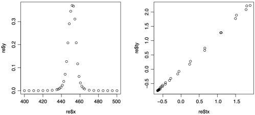
Figure 1:

Having computed $\hat{R}$, the estimate of $R$, we compute its significance under the null hypothesis of independence using the permutation distribution just as Szekely and Rizzo did. The $p$-value is ${\leq}0.001$, which is extremely small as it should be.

Table 1:

	$\bolds{K=2}$, $\bolds{L=2}$	$\bolds{K=3}$, $\bolds{L=4}$	$\bolds{K=5}$, $\bolds{L=5}$
Estimated ($K$,$L$) correlation	$0.8160803$	$0.9170764$	$0.977163$
$p$-value	$0.002$	$0.002$	${\leq}0.001$

Next, we compute the empirical $(K,L)$ correlation. Given that the proposed nonlinear model is

$$y=\frac{\beta_{1}}{\beta_{2}}\exp\biggl{\{}\frac{-(x-\beta_{3})^{2}}{2\beta_{2}^{2}}\biggr{\}}+\varepsilon,$$

we chose, as an orthonormal basis with respect to the Lebesgue measure, one defined by the Hermite polynomials defined as $H_{n}(x)=(-1)^{n}e^{x^{2}/2}\frac{d^{n}}{dx^{n}}e^{-x^{2}/2}$, for both $X$ and $Y$. We take $f_{k}(\cdot)=g_{k}(\cdot)=e^{-x^{2}/4}H_{k}(\cdot)$.

Table 1 gives the computation results of different combinations of $K$ and $L$. As before, the $p$-value is computed by a permutation test, based on $999$ replicates.

The value, not surprisingly, is close to $\hat{R}$, for $K=L=5$.

References

- (1) Bickel, P. J., Ritov, Y. and Stoker, T. M. (2006). Tailor-made tests for goodness of fit to semiparametric hypotheses. Ann. Statist. 34 721–741. \MR2281882
- (2) Breiman, L. and Friedman, J. H. (1985). Estimating optimal transformations for multiple regression and correlation. J. Amer. Statist. Assoc. 80 580–598. \MR0803258
- (3) Chen, A. and Bickel, P. J. (2005). Consistent independent component analysis and prewhitening. IEEE Trans. Signal Process. 10 3625–3632. \MR2239886
- (4) Feuerverger, A. and Mureika, R. A. (1977). The empirical characteristic function and its applications. Ann. Statist. 5 88–97. \MR0428584