Synchronized Andreev Transmission in SNS Junction Arrays

Abstract

We construct a nonequilibrium theory for the charge transfer through a diffusive array of alternating normal (N) and superconducting (S) islands comprising an SNSNS junction, with the size of the central S-island being smaller than the energy relaxation length. We demonstrate that in the nonequilibrium regime the central island acts as Andreev retransmitter with the Andreev conversions at both NS interfaces of the central island correlated via over-the-gap transmission and Andreev reflection. This results in a synchronized transmission at certain resonant voltages which can be experimentally observed as a sequence of spikes in the differential conductivity.

An array of alternating superconductor (S) - normal metal (N) islands is a fundamental laboratory representing a wealth of physical systems ranging from Josephson junction networks and layered high temperature superconductors to disordered superconducting films in the vicinity of the superconductor-insulator transition. Electronic transport in these systems is mediated by Andreev conversion of a supercurrent into a current of quasiparticles and vice versa at interfaces between the superconducting and normal regions Andreev . A fascinating phenomenon benchmarking this mechanism is the enhancement of the conductivity observed in a single SNS junction at matching voltages constituting an integer ($m$) fraction of the superconducting gap, $V=2\Delta/(em)$ SNSexp due to the effect of multiple Andreev reflection (MAR) MAR . The current-voltage characteristics of diffusive SNS junctions were studied in detail in Shumeiko ; Cuevas . Recent experimental findings 2DSNS ; 1DSNS ; Fritz posed the question about the transport properties of large arrays comprised of many SNS junctions.

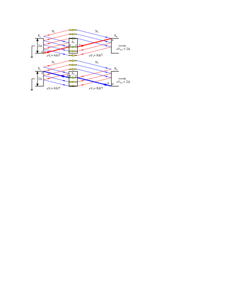
Figure 1: (color online). Diagrams of the SAT processes for $n=1$ in Eq. (1) in an SNSNS junction with normal resistance ratio $R_{1}/R_{2}=3/4$ (depicted through the 3/4 ratio of the respective lengths of the normal regions). The thick solid lines represent the synchronized quasiparticle paths connecting the points of singularity in the density of states corresponding to energies $\varepsilon=\pm\Delta$ at the electrodes S${}_{{}_{\mathrm{L}}}$ and S${}_{{}_{\mathrm{R}}}$. The paths ABCD (upper panel) and D^′C^′B^′A^′ (lower panel) correspond to the electron- and hole trajectories, respectively. Synchronization of the energies of the incident and emitted quasiparticles at points B and C (B^′ and C^′) is shown by arrows. SAT is realized by trajectories passing through the singular points $\pm\Delta$ of the central island S${}_{{}_{\mathrm{C}}}$ and including above-the-gap Andreev reflections. Trajectories synchronizing other transmissions across S${}_{{}_{\mathrm{C}}}$ and those of higher orders are not shown. Note, that voltage drops $eV_{1}=6\Delta/7$ and $eV_{2}=8\Delta/7$ are not MAR matching voltages of either the S${}_{{}_{\mathrm{L}}}$N₁S${}_{{}_{\mathrm{C}}}$ or the S${}_{{}_{\mathrm{C}}}$N₂S${}_{{}_{\mathrm{R}}}$ part.

In this Letter we develop a nonequilibrium theory for the current-voltage characteristics of a series of two diffusive SNS junctions, i.e. an SNSNS junction. The normal parts have, in general, different resistances and are coupled via a small superconducting granule, S${}_{{}_{\mathrm{C}}}$. The focal point is the construction of a nonequilibrium circuit theory for the charge transfer across the superconducting island. We demonstrate that the wedging of S${}_{{}_{\mathrm{C}}}$ into the normal part of an SNS junction leads to nontrivial physics and the appearance of a new distinct resonant mechanism for the current transfer: the Synchronized Andreev Transmission (SAT). In the SAT regime the processes of Andreev conversion at the boundaries of the central superconducting island are correlated: as a quasiparticle with energy $\varepsilon$ hits one NS${}_{{}_{\mathrm{C}}}$ interface, a quasiparticle with the same energy emerges from the other S${}_{{}_{\mathrm{C}}}$N interface into the bulk of the normal island (and vice versa, see Fig. 1). This energy synchronization is achieved via over-the-gap Andreev processes 1DSNS , which couple the MAR processes occurring in each of the normal islands and make the quasiparticle distributions at the central island essentially in nonequilibrium. Effectiveness of the synchronization is controlled by the energy relaxation lengths of both, the quasiparticles crossing S${}_{{}_{\mathrm{C}}}$ with energies above $\Delta$, and of quasiparticles experiencing MAR in the normal parts. The SAT processes result in spikes in the differential conductivity of the SNSNS circuit, which appear at resonant values of the total applied voltage $V_{\mathrm{tot}}$ defined by the condition

$$V_{\mathrm{tot}}=\frac{2\Delta}{en}$$ (1)

with integer $n$, irrespectively of the details of the distribution of the partial voltages at the two normal islands. As we show below, the SAT-induced features become dominant in large arrays consisting of many SNS junctions.

The model.— We consider the charge transfer across an S${}_{{}_{\mathrm{L}}}$N₁S${}_{{}_{\mathrm{C}}}$N₂S${}_{{}_{\mathrm{R}}}$ junction, where S${}_{{}_{\mathrm{L}}}$, S${}_{{}_{\mathrm{C}}}$, and S${}_{{}_{\mathrm{R}}}$ are superconducting islands with identical gap $\Delta$. We assume the size of the central island $L_{{}_{\mathrm{C}}}$ to be much larger than the superconducting coherence length $\xi$, hence processes of subgap elastic cotunneling and/or direct Andreev tunneling Deutcher are not effective. In general this condition ensures that $L_{{}_{\mathrm{C}}}$ is large enough so that charges do not accumulate in the central island and Coulomb blockade effects are irrelevant for the quasiparticle transport. At the same time $L_{{}_{\mathrm{C}}}$ is assumed to be less than the charge imbalance length, such that we can neglect the coordinate dependence of the quasiparticle distribution functions across the island S${}_{{}_{\mathrm{C}}}$. Additionally, the condition $\ell_{\varepsilon}\gg L_{{}_{\mathrm{C}}}$, where $\ell_{\varepsilon}$ is the energy relaxation length, implies that quasiparticles with energies $\varepsilon>\Delta$ traverse the central superconducting island S${}_{{}_{\mathrm{C}}}$ without a loss of energy. The normal parts N₁ and N₂ are the diffusive normal metals of length $L_{1,2}>\xi$, and $L_{1,2}>L_{{}_{\mathrm{T}}}$, $L_{{}_{\mathrm{T}}}=\sqrt{\hbar D_{{}_{\mathrm{N}}}/\varepsilon}$, where $D_{{}_{\mathrm{N}}}$ is the diffusion coefficient in the normal metal. We assume the Thouless energy, $E_{\mathrm{Th}}=\hbar D_{{}_{\mathrm{N}}}/L_{1,2}^{2}$, to be small, $E_{\mathrm{Th}}\ll\Delta$, and not to exceed the characteristic voltage drops, $E_{\mathrm{Th}}<eV_{1,2}$. These conditions are referred to as incoherent regime Shumeiko where, in particular, the Josephson coupling between the superconducting islands is suppressed. We let the energy relaxation length in the normal parts N₁ and N₂ be much larger than their sizes, thus quasiparticles may experience many incoherent Andreev reflections inside the normal regions.

The current transfer across the SNSNS junction is described by quasiclassical Larkin-Ovchinnikov (LO) equations for the dirty limit Larkin_Ovchinnikov :

$$-i[\check{H}_{\rm eff}\circ,{\bf\check{G}}]=\nabla\mathbf{\check{J}},\quad\check{\mathbf{J}}\cdot\mathbf{n}=\frac{1}{2\sigma_{{{}_{\mathrm{S}}}}R}[\check{G}_{{}_{\mathrm{S}}}\,,\check{G}_{{}_{\mathrm{N}}}]\,,$$ (2)

where $\check{H}_{\rm eff}=\check{1}(i\hat{\sigma}_{z}\partial_{t}-\varphi\hat{\sigma}_{0}+\hat{\Delta})$, $\mathbf{\check{J}}=D{\bf\check{G}}\circ\nabla{\bf\check{G}}$ is the matrix current, the subscripts “S” and “N” stand for superconducting and normal materials, respectively, “$\circ$” is the time-convolution, $\hat{\sigma}^{\alpha}$ ($\alpha=\{0,1,2,3\}$) are the Pauli matrices, $\hat{\Delta}=i\hat{\sigma}_{\mathrm{x}}\mathop{\mathrm{missing}}{Im}\nolimits\Delta+i\hat{\sigma}_{\mathrm{y}}\mathop{\mathrm{missing}}{Re}\nolimits\Delta$, and $R$ is the resistance of an NS interface. The diffusion coefficient $D$ assumes the value $D_{{}_{\mathrm{N}}}$ in the normal metal and the value $D_{{}_{\mathrm{S}}}$ in the superconductor, and $\varphi$ is the electrical potential which we calculate self-consistently. The unit vector $\mathbf{n}$ is normal to the NS interface and is assumed to be directed from N to S. The momentum averaged Green’s functions ${\bf\check{G}}({\bf r},t,t^{\prime})$ are $2\times 2$ matrices in a Keldysh space. Each element of the Keldysh matrix, labelled with a hat sign, is, in its turn, a $2\times 2$ matrix in the electron-hole space:

$${\bf\check{G}}=\left(\begin{array}[]{cc}\hat{G}^{\mathrm{R}}&\hat{G}^{\mathrm{K}}\\ 0&\hat{G}^{\mathrm{A}}\end{array}\right);\hskip 8.53581pt\hat{G}^{{\mathrm{R}}({\mathrm{A}})}=\left(\begin{array}[]{cc}{\cal G}^{{\mathrm{R}}({\mathrm{A}})}&{\cal F}^{{\mathrm{R}}({\mathrm{A}})}\\ \tilde{\cal F}^{{\mathrm{R}}({\mathrm{A}})}&\tilde{\cal G}^{{\mathrm{R}}({\mathrm{A}})}\end{array}\right)\,,$$ (3)

${\bf r}$ is the spatial position and $t$, $t^{\prime}$ are the two time arguments. The Keldysh component of the Green’s function is parametrized as Larkin_Ovchinnikov : $\hat{G}^{\mathrm{K}}=\hat{G}^{\mathrm{R}}\circ\hat{f}-\hat{f}\circ\hat{G}^{\mathrm{A}}$, where $\hat{f}$ is the distribution function matrix, diagonal in Nambu space, $\hat{f}\equiv\mathrm{diag}\,[1-2n_{\mathrm{e}},1-2n_{\mathrm{h}}]$, $n_{\mathrm{e(h)}}$ is the electron (hole) distribution function. In equilibrium $n_{\mathrm{e(h)}}$ becomes the Fermi function. And, finally, the Green’s function satisfies the normalization condition ${\bf\check{G}}^{2}=\check{1}$.

The edge conditions closing Eqs. (2) are given by the expressions for the Green’s functions in the bulk of the left (L) and right (R) superconducting leads:

$${\bf\check{G}}_{{\mathrm{L}}({\mathrm{R}})}(t,t^{\prime})=e^{-i\mu_{{\mathrm{L}}({{\mathrm{R}})}}t\hat{\tau}_{3}/\hbar}{\bf\check{G}}_{0}(t-t^{\prime})e^{i\mu_{{\mathrm{L}}({{\mathrm{R}})}}t^{\prime}\hat{\tau}_{3}/\hbar}\,,$$

the chemical potentials are $\mu_{{}_{\mathrm{L}}}=0$ and $\mu_{{}_{\mathrm{R}}}=eV$. Here, ${\bf\check{G}}_{0}(t)$ is the equilibrium bulk BCS Green’s function.

The current density is expressed through the Keldysh component of $\mathbf{\check{J}}$ as

$$\mathcal{I}(t,\mathbf{r})=\frac{\pi\sigma_{{}_{\mathrm{N}}}}{4}\operatorname{Tr}\hat{\sigma}_{z}\hat{J}^{\mathrm{K}}(t,t;\mathbf{r})=\frac{1}{2}\int d\varepsilon\left[I_{\mathrm{e}}(\varepsilon)+I_{\mathrm{h}}(\varepsilon)\right]\,,$$ (4)

where the spectral currents $I_{\mathrm{e}}$ and $I_{\mathrm{h}}$ are the time Wigner-transforms of top- and bottom diagonal elements of the matrix current $\mathbf{\check{J}}^{({\mathrm{K}})}$, representing electron and hole quasiparticle currents, respectively. In the bulk of a normal metal $I_{\mathrm{e}}=\sigma_{{}_{\mathrm{N}}}\nabla n_{\mathrm{e}}$ and $I_{\mathrm{h}}=\sigma_{{}_{\mathrm{N}}}\nabla n_{\mathrm{h}}$.

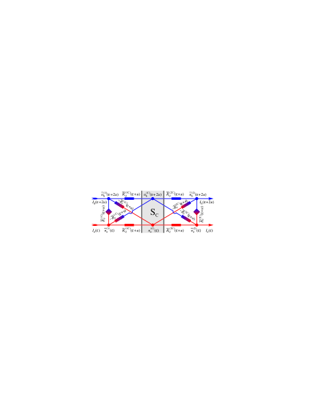
Figure 2: (color online). Effective circuit representing current conversion at the interfaces of the central superconducting island S${}_{{}_{\mathrm{C}}}$. Resistors, $R_{{}_{\mathrm{P}}}$ and $R_{{}_{\mathrm{Q}}}$ stand for an Andreev- and a normal processes, respectively.

The distribution functions of quasiparticles at the central island S${}_{{}_{\mathrm{C}}}$ are essentially is nonequilibrium. To take this into account we define quasiparticle spectral currents at NS interfaces by the Keldysh component of the boundary conditions for Eqs. (2). These nonequilibrium boundary conditions have a form of Kirchhoff’s laws for the circuit shown in Fig. 2. The electron and hole distribution functions take the role of voltages at the nodes. For illustration we write down the equation for an electronic spectral current flowing into the lower left corner node (Kirchhoff’s laws at the other corner nodes have a similar form):

$$I_{\mathrm{e}}(\varepsilon)=\frac{1}{\bar{R}_{{}_{\mathrm{Q}}}^{(\scriptscriptstyle{\mathrm{1C}})}(\varepsilon+u)}\left[n_{\mathrm{e}}^{{\scriptscriptstyle({\mathrm{C}})}}(\varepsilon)-\bar{n}_{\mathrm{e}}^{({1})}(\varepsilon)\right]-\\ \frac{1}{\bar{R}_{{}_{\mathrm{P}}}^{(\scriptscriptstyle{\mathrm{1C}})}(\varepsilon+u)}\,\left[{n}_{\mathrm{h}}^{{\scriptscriptstyle{(\mathrm{C}})}}(\varepsilon+2u)-\bar{n}_{\mathrm{e}}^{({1})}(\varepsilon)\right]+\\ \frac{1}{\bar{R}_{{}_{\mathrm{P}}}^{(\scriptscriptstyle{\mathrm{1C}})}(\varepsilon+u)}\,\left[\bar{n}_{\mathrm{h}}^{({1})}(\varepsilon+2u)-\bar{n}_{\mathrm{e}}^{({1})}(\varepsilon)\right]\,.$$ (5)

The interjacent resistances, $\bar{R}_{{{}_{\mathrm{Q}}({{}_{\mathrm{P}}})}}$, are defined as $\bar{R}_{{{}_{\mathrm{Q}}({{}_{\mathrm{P}}})}}^{-1}(\varepsilon)=\{\bar{R}^{-1}_{-}(\varepsilon)\pm\bar{R}^{-1}_{+}(\varepsilon)\}/2$ where $\bar{R}_{\pm}(\varepsilon)$ are the special functions characterizing transparencies of the interfaces and tabulated in Shumeiko . At high energies, $|\varepsilon|\gg\Delta$, $\bar{R}_{+}(\varepsilon)\to\bar{R}_{-}(\varepsilon)$; at small energies, $|\varepsilon|\ll\Delta$, $\bar{R}_{-}(\varepsilon)$ diverges, while $\bar{R}_{+}(\varepsilon)-\bar{R}_{-}(\varepsilon)$ remains finite; and there are singularities in $\partial_{\varepsilon}\bar{R}_{\pm}(\varepsilon)$ at $|\epsilon|=\Delta$, which are of the same origin as those in the BCS density of states and reflect the fact that quasiparticles cannot penetrate the superconductor below the gap. The “bars” indicate that the respective resistances and the distribution functions are renormalized by the proximity effect.

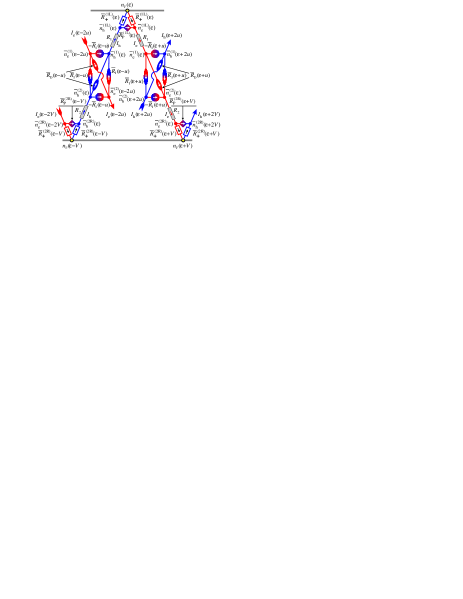
Figure 3: (color online). Effective circuit for an SNSNS junction. To simplify the graph, resistors $\bar{R}_{{{}_{\mathrm{D}}({{}_{\mathrm{I}}})}}^{-1}=(1/2)\{[\bar{R}_{+}^{({{\scriptscriptstyle{\mathrm{1C}}}})}+\bar{R}_{+}^{({{\scriptscriptstyle{\mathrm{2C}}}})}]^{-1}\pm[\bar{R}_{-}^{({{\scriptscriptstyle{\mathrm{1C}}}})}+\bar{R}_{-}^{({{\scriptscriptstyle{\mathrm{2C}}}})}]^{-1}\}$ representing Andreev and normal processes at the NS interfaces of the central island are introduced.

To derive the current-voltage characteristics for the general case of an asymmetric nonequilibrium SNSNS junction with different resistances of the normal regions, we construct a nonequilibrium circuit theory allowing for an analytical solution of the nonlinear nonuniform matrix Eqs. (2) for Keldysh-Nambu Green’s functions. The diagrammatic mapping of Eqs. (2) is realized by an equivalent circuit shown in Fig. 3. The Kirchhoff’s equations for the potential distribution in the circuit of Fig. 3, give the recurrent relations:

$$\begin{split}\mathcal{R}(\varepsilon,-{\mathrm{u}},-V)I_{\mathrm{h}}(\varepsilon)-\rho^{(\circ)}({\varepsilon-{\mathrm{u}}})I_{\mathrm{e}}(\varepsilon-2{\mathrm{u}})\\ -\rho^{(\triangleright)}(\varepsilon)I_{\mathrm{e}}(\varepsilon)-\rho^{(\triangleleft)}(\varepsilon-V)I_{\mathrm{e}}(\varepsilon-V)\\ =n_{\scriptscriptstyle{\mathrm{F}}}(\varepsilon)-n_{\scriptscriptstyle{\mathrm{F}}}(\varepsilon-V),\end{split}$$ (6)

$$\begin{split}\mathcal{R}(\varepsilon,{\mathrm{u}},V)I_{\mathrm{e}}(\varepsilon)-\rho^{(\circ)}(\varepsilon+{\mathrm{u}})I_{\mathrm{h}}(\varepsilon+2{\mathrm{u}})\\ -\rho^{(\triangleright)}(\varepsilon)I_{\mathrm{h}}(\varepsilon)-\rho^{(\triangleleft)}(\varepsilon+V)I_{\mathrm{h}}(\varepsilon+2V)\\ =n_{\scriptscriptstyle{\mathrm{F}}}(\varepsilon+V)-n_{\scriptscriptstyle{\mathrm{F}}}(\varepsilon)\,,\end{split}$$ (7)

where the electric potential $u$ of the S_C island is calculated self-consistently from the electroneutrality condition, $u=(\pi/8)\operatorname{Tr}\hat{G}^{\scriptscriptstyle{\mathrm{K}}}$. The effective resistance is $\mathcal{R}=R_{{1}}+R_{2}+\rho^{(\triangleright\circ\triangleleft)}$, where $\rho^{(\triangleright\circ\triangleleft)}=(1/2)\sum_{\alpha=\pm}\{\bar{R}_{\alpha,\varepsilon}^{({{\scriptscriptstyle{\mathrm{1L}}}})}+\bar{R}_{\alpha,\varepsilon+{\mathrm{u}}}^{({{\scriptscriptstyle{\mathrm{1C}}}})}+\bar{R}_{\alpha,\varepsilon+{\mathrm{u}}}^{({{\scriptscriptstyle{\mathrm{2C}}}})}+\bar{R}_{\alpha,\varepsilon+\scriptscriptstyle{\mathrm{V}}}^{({{\scriptscriptstyle{\mathrm{2R}}}})}\}$, $\rho^{(\circ)}=(1/2)\{\bar{R}_{+}^{({{\scriptscriptstyle{\mathrm{1C}}}})}+\bar{R}_{+}^{({{\scriptscriptstyle{\mathrm{2C}}}})}-\bar{R}_{-}^{({{\scriptscriptstyle{\mathrm{1C}}}})}-\bar{R}_{-}^{({{\scriptscriptstyle{\mathrm{2C}}}})}\}$, $\rho^{(\triangleleft)}=(1/2)\{\bar{R}_{+}^{({{\scriptscriptstyle{\mathrm{2R}}}})}-\bar{R}_{-}^{({{\scriptscriptstyle{\mathrm{2R}}}})}\}$, and $\rho^{(\triangleright)}=(1/2)\{\bar{R}_{+}^{({{\scriptscriptstyle{\mathrm{1L}}}})}-\bar{R}_{-}^{({{\scriptscriptstyle{\mathrm{1L}}}})}\}$. Solutions of Eqs.(6) yield the required $I$-$V$ characteristics for an asymmetric SNSNS junction. To verify our formulas we note that at large quasiparticle energies, $|\varepsilon|\gg\Delta$, the total resistance $\mathcal{R}$ reduces to the normal resistance of the array, whereas $\rho^{(\triangleleft)}$ and $\rho^{(\triangleright)}$ vanish. Then we find from Eqs.(6)-(7) that $I_{\mathrm{h}}(\varepsilon)=[n_{\scriptscriptstyle{\mathrm{F}}}(\varepsilon)-n_{\scriptscriptstyle{\mathrm{F}}}(\varepsilon-V)]/\mathcal{R}$, and $I_{\mathrm{e}}(\varepsilon)=[n_{\scriptscriptstyle{\mathrm{F}}}(\varepsilon+V)-n_{\scriptscriptstyle{\mathrm{F}}}(\varepsilon)]/\mathcal{R}$, which together with Eq.(4) reproduce Ohm’s law, $\mathcal{I}=V/\mathcal{R}$. The constructed diagram, Fig. 3, is an elemental building unit for a general nonequilibrium quantitative theory of SNS arrays comprised of many SNS junctions.

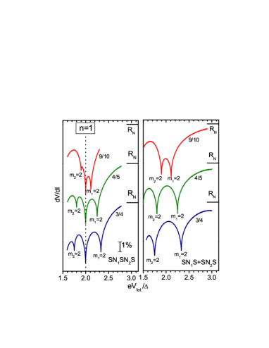
Figure 4: (color online). Left panel: Differential resistances as functions of the applied voltage $V_{\mathrm{tot}}$ (around $n=1$ in Eq. (1)) for the SN₁SN₂S junction. The fractions 3/4, and 4/5, and 9/10 represent the ratios of resistances of the normal regions, $R_{1}/R_{2}$. $dV/dI$ of SN₁SN₂S junction demonstrates the pronounced SAT spike at $V_{\mathrm{tot}}=2\Delta/e$, irrespectively of the partial voltage drops. The SAT spike is sandwiched between the two additional spikes corresponding to individual MAR processes occurring at junctions SN₁S and SN₂S for $m_{1},m_{2}=2$. The voltage positions of these features depends on $R_{1}/R_{2}$. Right panel: The corresponding $dV/dI(V_{1}+V_{2})$ for two SN₁S and SN₂S junctions in series as they would have appeared in absence of the synchronization process, i.e. when $L_{\scriptscriptstyle{\mathrm{C}}}>\ell_{\varepsilon}$. These $dV/dI$ were calculated following Shumeiko (with transmissivity W=1).

Results and discussion.— The calculation of the current-voltage characteristics ${\mathcal{I}}(V)$ requires the numerical solution of the recurrent relations, Eqs. (6)-(7). To this end, we have developed a computational scheme allowing to bypass instabilities caused by the non-analytic behavior of the spectral currents $I_{{\mathrm{e}}({\mathrm{h}})}(\varepsilon)$. We first fix some chosen energy $\varepsilon$, identify the set of energies connected through the equations in the given energy interval, and solve the resulting subsystem of equations. We then repeat the procedure, until the required energy resolution of $\delta\varepsilon=10^{-5}\Delta$ is achieved. Typically, up to $10^{6}$ linear equations had to be solved for every given voltage, but the complexity of the coupled subsystem depends on the commensurability of $u$ and $V$.

Figure 4 shows the comparative results for the SNSNS junction and two SNS junctions in series. The latter corresponds to the case where the size of the central island well exceeds the energy relaxation length, $L_{\scriptscriptstyle{\mathrm{C}}}>\ell_{\varepsilon}$. We display the differential resistances as functions of the applied voltage, which demonstrate the singularities in Andreev transmission more profoundly than the $I$-$V$ curves. There is a pronounced SAT spike in the $dV/dI$ for an SNSNS junction at $V_{\mathrm{tot}}=2\Delta/e$. The spike appears irrespectively of the partial voltage drops in the normal regions and is absent in the corresponding curves representing two individual MAR processes at the junctions SN₁S and SN₂S.

The resonant voltages of the SAT singularities can be found from the consideration of the quasiparticle trajectories in the space-energy diagrams. Such a diagram for the first subharmonic, $n=1$ and ratio $R_{1}/R_{2}=3/4$ is given in Fig. 1. A quasiparticle starts from the left superconducting electrode with the energy $\varepsilon=-\Delta$ to traverse N₁, and the quasiparticle that starts from the central island S_c with the same energy as the incident one to take up upon the current across the island N₂, and hit S_R with the energy $\varepsilon=\Delta$ (the ABCD path, the corresponding path for the hole is D^′C^′B^′A^′). In general, relevant trajectories yielding resonant voltages of Eq. (1) have the following structure: they start and end at the BCS quasiparticle density of states singular points ($\varepsilon=\pm\Delta$), contain the closed polygonal path, which include MAR staircases in the normal parts and over-the-gap transmissions and Andreev reflections, and pass the density of states singular points at the central island. Apart from the main singularities [Eq. (1)], additional SAT satellite spikes appear at $V=(2\Delta/e)(p+q)/n$, where $p/q$ is the irreducible rational approximation of the real number $r=R_{1}/R_{2}$, (we take $R_{1}<R_{2}$), and $n\geqslant(p+q)$.

The achieved qualitative understanding enables us to observe that the manifestations of the SAT mechanism in an experimental situation becomes even more pronounced with the growth of the number of SNS junctions in the system. To see this, let us assume that the resistances of the normal islands in a chain of SNS junctions are randomly scattered around their average value $R_{0}$ and follow Gaussian statistics with the standard deviation $\sigma_{\scriptscriptstyle{\mathrm{R}}}=\sigma R_{0}$, where $\sigma$ is dimensionless. Accordingly, the dispersion of the distribution of the MAR resonant voltages is characterized by the same $\sigma$, and the MAR features get smeared. Let us distribute the voltage drop $2\Delta/e$ among the $n$ successive islands. Then the quasiparticle SAT path starts at the lower edge of the superconducting gap at island $j$, traverses $n-1$ intermediate superconducting islands and hits the edge of the gap at the $j+n$-th island in the chain. The standard deviation of the voltage drop on the $n$ islands grows as $\sqrt{n}$ resulting in a voltage deviation per one island $\propto 1/\sqrt{n}$, i.e. the dispersion of the distribution of $V_{\mathrm{n}}$ drops with increasing $n$: $\sigma_{\scriptscriptstyle{\mathrm{SAT}}}=\sigma/\sqrt{n}$. In contrast to the MAR-induced features, with an increase of $n$, the subharmonic spikes at voltages $V_{\mathrm{n}}$ per junction due to SAT processes become more sharp and pronounced.

In conclusion, we have developed a nonequilibrium theory of charge transfer across a superconducting island and found that the island acts as Andreev retransmitter. We have shown that the nonequilibrium transport through an SNSNS array is governed by synchronized Andreev transmission with correlated conversion processes at the NS interfaces. The constructed theory is a fundamental building unit for a general quantitative description of a large array consisting of many SNS junctions.

References

- (1) A. F. Andreev, Zh. Eksp. Teor. Fiz. 46 (1964) 1823 [Sov. Phys. JETP 19 (1964) 1228].
- (2) J. M. Rowell and W. E. Feldmann, Phys. Rev. 172, 393 (1968); P. E. Gregers-Hansen et al., Phys. Rev. Lett. 31, 524 (1973); W. M. van Huffelen et al., Phys. Rev. B 47, 5170 (1993); A. W. Kleinsasseret al., Phys. Rev. Lett. 72, 1738 (1994); E. Scheer et al., Phys. Rev. Lett. 78, 3535 (1997); J. Kutchinsky et al., Phys. Rev. Lett. 78, 931 (1997); A. Frydman and R. C. Dynes, Phys. Rev. B 59, 8432 (1999); T. Hoss et al., Phys. Rev. B 62, 4079 (2000); T. I. Baturina et al., Physica B 284, 1860 (2000); Z. D. Kvon et al., Phys. Rev. B 61, 11340 (2000).
- (3) T. M. Klapwijk, G. E. Blonder, and M. Tinkham, Physica B+C (Amsterdam) 110, 1657 (1982).
- (4) E. V. Bezuglyi et al., Phys. Rev. B 62, 14439 (2000). In this work superconductors were considered to be in a local equilibrium and the relation was satisfied. This approach was further developed by N. M. Chtchelkatchev, JETP Lett. 83, 250 (2005); however in case of geometrically non-symmetric SNS arrays, it results in an equivalent circuit with the ennumerable number of elements.
- (5) J. C. Cuevas et al., Phys. Rev. B 73, 184505 (2006).
- (6) T. I. Baturina et al., Phys. Rev. B 63, 180503(R) (2001); JETP Lett. 81, 10 (2005).
- (7) T. I. Baturina et al., JETP Lett. 75, 326 (2002).
- (8) J. Fritzsche, R. B. G. Kramer, and V. V. Moshchalkov, Phys. Rev. B 80, 094514 (2009).
- (9) G. Deutscher and D. Feinberg, Appl. Phys. Lett. 76, 487 (2000).
- (10) A.I. Larkin and Yu.N. Ovchinnikov, Sov. Phys. JETP 41, 960 (1975); ibid, 46, 155 (1977).