How Do Massive Black Holes Get Their Gas?

Abstract

We use multi-scale smoothed particle hydrodynamic simulations to study the inflow of gas from galactic scales ($\sim 10\,$kpc) down to $\lesssim 0.1\,$pc, at which point the gas begins to resemble a traditional, Keplerian accretion disk. The key ingredients of the simulations are gas, stars, black holes (BHs), self-gravity, star formation, and stellar feedback (via a subgrid model); BH feedback is not included. We use $\sim 100$ simulations to survey a large parameter space of galaxy properties and subgrid models for the interstellar medium physics. We generate initial conditions for our simulations of galactic nuclei ($\lesssim 300$ pc) using galaxy scale simulations, including both major galaxy mergers and isolated bar-(un)stable disk galaxies. For sufficiently gas-rich, disk-dominated systems, we find that a series of gravitational instabilities generates large accretion rates of up to $\sim 1-10\,M_{\sun}\,{\rm yr^{-1}}$ onto the BH (i.e., at $\lesssim 0.1$ pc); this is comparable to what is needed to fuel the most luminous quasars. The BH accretion rate is highly time variable for a given set of conditions in the galaxy at $\sim$ kpc. At radii $\gtrsim 10$ pc, our simulations resemble the “bars within bars” model of Shlosman et al, but we show that the gas can have a diverse array of morphologies, including spirals, rings, clumps, and bars; the duty cycle of these features is modest, complicating attempts to correlate BH accretion with the morphology of gas in galactic nuclei. At $\sim 1-10$ pc, the gravitational potential becomes dominated by the BH and bar-like modes are no longer present. However, we show that the gas can become unstable to a standing, eccentric disk or a single-armed spiral mode ($m=1$), in which the stars and gas precess at different rates, driving the gas to sub-pc scales (again for sufficiently gas-rich, disk-dominated systems). A proper treatment of this mode requires including star formation and the self-gravity of both the stars and gas (which has not been the case in many previous calculations). Our simulations predict a correlation between the BH accretion rate and the star formation rate at different galactic radii. We find that nuclear star formation is more tightly coupled to AGN activity than the global star formation rate of a galaxy, but a reasonable correlation remains even for the latter.

1 Introduction

The inflow of gas into the central parts of galaxies plays a critical role in galaxy formation, ultimately generating phenomena as diverse as bulges and spheroidal galaxies, starbursts and ultra-luminous infrared galaxies (ULIRGs), nuclear stellar clusters, and accretion onto super-massive black holes (BHs). The discovery, in the past decade, of tight correlations between black hole mass and host spheroid properties including mass (Kormendy & Richstone, 1995; Magorrian et al., 1998), velocity dispersion (Ferrarese & Merritt, 2000; Gebhardt et al., 2000), and binding energy or potential well depth (Hopkins et al., 2007; Aller & Richstone, 2007) implies that these phenomena are tightly coupled.

It has long been realized that bright, high-Eddington ratio accretion (i.e., a quasar) dominates the accumulation of mass in the supermassive BH population (Soltan, 1982; Salucci et al., 1999; Shankar et al., 2004). In order to explain the existence of black holes with masses $\sim 10^{9}M_{\odot}$, the amount of gas required is comparable to that contained in entire large galaxies. Given the short lifetime of the quasar phase $\lesssim\,10^{8}\,{\rm yr}$ (Martini, 2004), the processes of interest must deliver a galaxy’s worth of gas to the inner regions of a galaxy on a relatively short timescale.

There is also compelling evidence that quasar activity is preceded and/or accompanied by a period of intense star formation in galactic nuclei (Sanders et al., 1988a, b; Dasyra et al., 2007; Kauffmann et al., 2003). The observed properties of bulges at $z\sim 0$ independently require that dissipative processes (gas inflow) dominate the formation and structure of the inner $\sim$kpc (Ostriker, 1980; Carlberg, 1986; Gunn, 1987; Kormendy, 1989; Hernquist et al., 1993). Hopkins et al. (2009a, d, 2008a) showed that this inner dissipational component can constitute a large fraction $\sim 5-30\%$ of the galaxy’s mass, with stellar (and at some point probably gas) surface densities reaching $\sim 10^{11-12}\,M_{\sun}\,{\rm kpc^{-2}}$.

On large (galactic) scales, several viable processes for initiating such inflows are well-known. Major galaxy-galaxy mergers produce strong non-axisymmetric disturbances of the constituent galaxies; such disturbances may also be produced in some minor mergers and/or globally self-gravitating isolated galactic disks. Observationally, major mergers are associated with enhancements in star formation in ULIRGs, sub-millimeter galaxies, and pairs more generally (e.g. Sanders & Mirabel, 1996; Schweizer, 1998; Jogee, 2006; Dasyra et al., 2006; Woods et al., 2006; Veilleux et al., 2009). Numerical simulations of mergers have shown that when such events occur in gas-rich galaxies, resonant tidal torques lead to rapid inflow of gas into the central $\sim\,$kpc (Hernquist, 1989; Barnes & Hernquist, 1991, 1996). The resulting high gas densities trigger starbursts (Mihos & Hernquist, 1994, 1996), and are presumed to feed rapid black hole growth. Feedback from the starburst and a central active galactic nucleus (AGN) may also be important, both for regulating the BH’s growth (Di Matteo et al., 2005; Hopkins et al., 2005; DeBuhr et al., 2009; Johansson et al., 2009b) and for shutting down future star formation (Springel et al. 2005a; Johansson et al. 2009a; see, however, DeBuhr et al. 2009).

However, the physics of how gas is transported from $\sim 1$ kpc to much smaller scales remains uncertain (e.g., Goodman 2003). Typically, once gas reaches sub-kpc scales, the large-scale torques produced by a merger and/or large-scale bar/spiral become less efficient. In the case of stellar bars or spiral waves, there can even be a “hard” barrier to further inflow in the form of an inner Linblad resonance, if the system has a non-trivial bulge. In mergers, the coalescence of the two systems generates perturbations on all scales, and so allows gas to move through the resonances, but the perturbations relax rapidly on small scales, often before gas can inflow.

Local viscous stresses – which are believed to dominate angular momentum transport near the central BH (e.g., Balbus & Hawley 1998) – are inefficient at radii $\gtrsim 0.01-0.1$ pc (e.g., Shlosman & Begelman 1989; Goodman 2003; Thompson et al. 2005). It is in principle possible that some molecular clouds could be scattered onto very low angular momentum orbits, but even the optimistic fueling rates from this process are generally insufficient to produce luminous quasars (see e.g. Hopkins & Hernquist, 2006; Kawakatu & Wada, 2008; Nayakshin & King, 2007). As a consequence, many models invoke some form of gravitational torques (“bars within bars”; Shlosman et al. 1989) to continue transport to smaller radii. As gas is driven into the central kpc by large-scale torques, it will cool rapidly into a disky structure; if this gas reservoir is massive enough, the gas will be self-gravitating and thus again vulnerable to global instabilities (e.g., the well-known bar and/or spiral wave instabilities) that can drive some of the gas to yet smaller radii.

To date, numerical simulations have seen the formation of such secondary bars in some circumstances, such as in adaptive mesh refinement (AMR) simulations of galaxy formation (Wise et al., 2007; Levine et al., 2008; Escala, 2007) or particle-splitting smoothed particle hydrodynamics (SPH) simulations of some idealized systems (Escala et al., 2004; Mayer et al., 2007). These studies have served as a critical “proof of concept.” However, these examples have generally been limited by computational expense to studying a single system at one instant in its evolution, and thus it is difficult to assess how the sub-pc dynamics depends on the large parameter space of possible inflow conditions from large radii and galaxy structural parameters.

Alternatively, some simulations simply take an assumed small-scale structure and/or fixed inflow rate as an initial/boundary condition, and study the resulting gas dynamics at small radii (e.g. Schartmann et al., 2009; Dotti et al., 2009; Wada & Norman, 2002; Wada et al., 2009). These studies have greatly informed our understanding of nuclear obscuration on small scales (the “torus”), and the role of stellar feedback in determining the structure and dynamics of the gas at these radii; it is, however, unclear how to relate this small-scale dynamics to the larger-scale properties of the host galaxy. This is critical for understanding black hole growth and nuclear star formation in the broader context of galaxy formation.

Observationally, a long standing puzzle has been that many systems, especially those with weaker inflows on large scales (e.g. bar or spiral wave-unstable disks with some bulge, as opposed to major mergers), exhibit no secondary instabilities at $\sim 0.1-1$ kpc – in several cases, torques clearly reverse sign inside these radii (Block et al., 2001; García-Burillo et al., 2005). Whether this is generic, or the consequence of a low duty cycle, or the result of the large-scale inflows simply being too weak in these cases, is not clear. Moreover, even among systems that do show nuclear asymmetries, and that clearly exhibit enhanced star formation and luminous AGN, the observed features at smaller radii are very often not traditional bars. Rather, they exhibit a diverse morphology, with spirals quite common, along with nuclear rings, barred rings, occasional one or three-armed modes, and some clumpy/irregular structures (Martini & Pogge, 1999; Peletier et al., 1999; Knapen et al., 2000; Laine et al., 2002; Knapen et al., 2002; Greene et al., 2009).

Even if secondary bars or spirals are present at intermediate radii $\sim 10-100$ pc, it has long been recognized that they will cease to be important at yet smaller scales, when the potential becomes quasi-Keplerian and the global self-gravity of the gas less important; this occurs as one approaches the BH radius of influence, which is $\sim 10\,$pc in typical $\sim L_{\ast}$ galaxies (Athanassoula et al., 1983, 2005; Shlosman et al., 1989; Heller et al., 2001; Begelman & Shlosman, 2009). Indeed, in previous simulations and most analytic calculations, the “bars-within-bars” model appears to break down at these scales (see e.g. Jogee, 2006, and references therein). However, local angular momentum transport is still very inefficient at $\sim 10$ pc, and the gas is still locally self-gravitating, and so should be able to form stars rapidly (e.g., Thompson et al. 2005). Understanding the physics of inflow through these last few pc, especially in a consistent model that connects to gas on galactic scales ($\sim 10\,$kpc), remains one of the key open questions in our understanding of massive BH growth.

In this paper, we present a suite of multi-scale hydrodynamic simulations that follow gravitational torques and gas inflow from the kpc scales of galaxy-wide events through to $<0.1\,$pc where the material begins to form a standard thin accretion disk. These simulations include gas cooling, star formation, and self-gravity; feedback from supernovae and stellar winds is crudely accounted for via a subgrid model. In order to isolate the physics of angular momentum transport, we do not include BH feedback in our calculations. We systematically survey a large range of galaxy properties (e.g., gas fraction and bulge to disk ratio) and gas thermodynamics, in order to understand how these influence the dynamics, inflow rates, and observational properties of gas on small scales in galactic nuclei ($\sim 0.1-100$ pc). Our focus in this paper is on the results of most observational interest: what absolute inflow rates, star formation rates, and gas/stellar surface density profiles result from secondary gravitational instabilities? What is their effective duty cycle? And what range of observational morphologies are predicted? In a future paper (Paper II) we will present a more detailed comparison between our numerical results and analytic models of inflow and angular momentum transport induced by non-axisymmetric instabilities in galactic nuclei.

The remainder of this paper is organized as follows. In § 2 we describe our simulation methodology, which consists of two levels of “re-simulations” using initial conditions motivated by galactic-scale simulations. In § 3 we present an overview of our results and show how a series of gravitational processes leads to gas transport from galactic scales to sub-pc scales. In §4 we quantify the resulting inflow rates and gas properties as a function of time and radius in the simulations. §5 summarizes the conditions required for global gravitational instability and significant gas inflow. In § 6 we show how the physics of accretion induced by gravitational instabilities leads to a correlation (with significant scatter) between star formation at different radii and BH accretion; we also compare these results to observations. In § 7 we summarize our results and discuss a number of their implications and several additional observational tests. Further numerical details and tests of our methodology are discussed in § A. In § B we show how the subgrid model of the ISM we use influences our results.

2 Methodology

We use a suite of hydrodynamic simulations to study the physics of gas inflow from $\sim 10\,$kpc to $\sim 0.1\,$pc in galactic nuclei. In order to probe the very large range in spatial and mass scales, we carry out a series of “re-simulations.” First, we simulate the dynamics on galaxy scales. Specifically, we use representative examples of gas-rich galaxy-galaxy merger simulations and isolated, moderately bar-unstable disk simulations. These are well-resolved down to $\sim 100-500\,$pc. We use the conditions at these radii (at several times) as the initial conditions for intermediate-scale re-simulations of the sub-kpc dynamics. In these re-simulations, the smaller volume is simulated at higher resolution, allowing us to resolve the subsequent dynamics down to $\sim 10\,$pc scales – these re-simulations approximate the nearly instantaneous behavior of the gas on sub-kpc scales in response to the conditions at $\sim$kpc set by galaxy-scale dynamics. We then repeat our re-simulation method to follow the dynamics down to sub-pc scales where the gas begins to form a standard accretion disk.

Our re-simulations are not intended to provide an exact realization of the small-scale dynamics of the larger-scale simulation that motivated the initial conditions of each re-simulation (in the manner of particle-splitting or adaptive-mesh refinement techniques). Rather, our goal is to identify the dominant mechanism(s) of angular momentum transport in galactic nuclei and what parameters they depend on. This approach clearly has limitations, especially at the outer boundaries of the simulations; however, it also has a major advantage. By not requiring the conditions at small radii to be uniquely set by a larger-scale “parent” simulation, we can run a series of simulations with otherwise identical conditions (on that scale) but systematically vary one parameter (e.g., gas fraction or ISM model) over a large dynamic range. This allows us to identify the physics and galaxy properties that have the biggest effect on gas inflow in galactic nuclei. As we will show, the diversity of behaviors seen in the simulations, and desire to marginalize over the uncertain ISM physics, makes such a parameter survey critical.

This methodology is discussed in more detail below. First, we describe the physics in our simulations, in particular our treatment of gas cooling, star formation, and feedback from supernovae and young stars (§ 2.1). We then summarize the galaxy-scale simulations that are used to motivate the initial conditions for subsequent re-simulations (§ 2.2). The intermediate-scale re-simulations, and the methodology used to construct their initial conditions, are discussed in § 2.3. Finally, we discuss the nuclear-scale resimulations, which are themselves motivated by the intermediate-scale resimulations (§ 2.4).

2.1 Gas Physics, Star Formation, and Stellar Feedback

Figure 1: Effective equation of state of the ISM in our simulations; this accounts for the effects of stellar feedback that are not resolved in our calculations. We plot the effective sound speed $c_{s}$ (i.e., the turbulent speed generated by feedback) versus average ISM density $n$. The $q_{\rm eos}=0$ case is an isothermal “floor” at $c_{s}=10\,{\rm km\,s^{-1}}$. The $q_{\rm eos}=1$ line is the “maximal feedback” model in Springel & Hernquist (2003), in which the ISM is multi-phase above a minimum $n$ and all supernova energy goes into pressurizing the “diffuse” medium. Intermediate $q_{\rm eos}$ interpolate between the two (eq. 1). For each $q_{\rm eos}$, we show an analytic curve for the equilibrium $c_{s}(n)$, and simulation results (colored points). We compile measurements of the turbulent or non-thermal velocities in observed systems (black points): local ULIRGs (Downes & Solomon, 1998, circles; large/small for the inner/outer observed radii in each), the nuclei of merging LIRGs (Bryant & Scoville, 1999, star), the core of M82 (Westmoquette et al., 2007, $\times$), the central 400 pc of NGC 6240 (Tacconi et al., 1999, triangle), nuclear clumps in NGC 6240 (Iono et al., 2007, pentagon), and the maser disk of NGC 3079 (Kondratko et al., 2005, small squares). The canonical spiral disk velocity dispersion is also shown (large square). At high-redshifts, we show recent observations of “normal” star-forming disks from Förster Schreiber et al. (2006, $z\sim 2$; diamond) and Lemoine-Busserolle et al. (2009, $z=3-4$; asterisk), and luminous sub-millimeter galaxies from Tacconi et al. (2006, inverted triangle). The observations favor a median $q_{\rm eos}\sim 0.125-0.3$, which we adopt as our “fiducial” models.

The simulations were performed with the parallel TreeSPH code GADGET-3 (Springel, 2005), based on a fully conservative formulation of smoothed particle hydrodynamics (SPH), which conserves energy and entropy simultaneously even when smoothing lengths evolve adaptively (see e.g., Springel & Hernquist, 2002; Hernquist, 1993; O’Shea et al., 2005). The detailed numerical methodology is described in Springel (2005), Springel & Hernquist (2003), and Springel et al. (2005b).

The simulations include supermassive black holes (BHs) as additional collisionless particles at the centers of all progenitor galaxies. In our calculations the BH’s only dynamical role is via its gravitational influence on the smallest scales $\sim 1-10$ pc. In particular, to cleanly isolate the physics of gas inflow, we do not include the subgrid models for BH accretion and feedback that have been used in previous works (e.g., Springel et al. 2005b). During a galaxy merger, the BHs in each galactic nucleus are assumed to coalesce and form a single BH at the center of mass of the system once they are within a single SPH smoothing length of one another and are moving at a relative speed lower than both the local gas sound speed and relative escape velocities.

In our models, stars form from the gas using a prescription motivated by the observed Kennicutt (1998) relation. Specifically, we use a star formation rate per unit volume $\dot{\rho}_{\ast}\propto\rho^{3/2}$ with the normalization chosen so that a Milky-way like galaxy has a total star formation rate of about $1\,M_{\sun}\,{\rm yr^{-1}}$.

The precise slope, normalization, and scatter of the Schmidt-Kennicutt relation, and even whether or not such a relation is generally applicable, are somewhat uncertain on the smallest spatial scales we model here. This is especially true when the dynamical times become short relative to the main-sequence stellar lifetime ($t_{\rm dyn}\sim 10^{5}-10^{6}\,$yr in the smallest regions simulated). Nonetheless, there is some observational and physical motivation for the “standard” parameters we have adopted, even at high surface densities. For the densest star forming galaxies, observational studies favor a logarithmic slope $\simeq 1.7$ for the relation between $\dot{\Sigma}_{*}$ and $\Sigma_{g}$ (Bouché et al., 2007), not that different from what our model implements. In addition, Tan et al. (2006) and Krumholz & Tan (2007) show that local observations imply a constant star formation efficiency in units of the dynamical time (i.e. $\dot{\rho}_{\ast}\propto\rho^{1.5}$) at all densities observed, $n\sim 10^{1-6}\,{\rm cm^{-3}}$ – the highest gas densities in these studies are comparable to the highest gas densities in our simulations ($\sim 10^{8}\,M_{\sun}$ of gas inside $\sim 10$ pc). Finally, Davies et al. (2007) & Hicks et al. (2009) estimate the star formation rate (SFR) and gas surface densities in AGN on exactly the small scales of interest here ($\sim 1-10\,$pc); they find a SFR-density relation continuous with that implied at “normal” galaxy densities.

To understand the possible impact of uncertainties in the Schmidt-Kennicutt relation on our conclusions, we have adjusted the slope ${\rm d}\ln\dot{\rho}_{\ast}/{\rm d}\ln\rho$ adopted in our simulations between $1.0-2.0$ in a small set of test runs, fixing the star formation rate at MW-like surface densities of $\simeq 10^{9}\,M_{\sun}\,{\rm kpc^{-2}}$ where the observational constraints are tight. This amounts to varying the absolute star formation efficiency on the smallest resolved scales by a factor of $\gtrsim 100$; qualitatively, this could presumably mimic a wide variety of different physics associated with stellar feedback and star formation. This variation can, unsurprisingly, have a dramatic affect on the quasi-equilibrium gas densities at small radii, which are set by gas inflow balancing star formation. However, even over this large range of star formation efficiencies, the qualitative behavior of the angular momentum transport and gas inflow does not change dramatically; the gas dynamics in a low-star formation efficiency run is similar to that in a run with much higher initial gas content but also higher star formation efficiency. As a result, although the absolute star formation efficiency is clearly somewhat uncertain, we do not believe that this qualitatively affects our conclusions.

The largest uncertainties in our modeling stem from the treatment of the interstellar medium (ISM) gas physics and the impact of stellar feedback on the ISM. Our simulations are relatively coarse and average over many star-forming clumps, HII regions, supernova remnants, etc. As a result, the simulations use a sub-resolution model of a multiphase ISM in which the gas has a sound speed much larger than its true thermal velocity (Springel & Hernquist, 2003). Our assumption is that the large-scale gravitational torques produced by bars, spiral waves, and other non-axisymmetric features, will not depend critically on the small-scale structure of the ISM; although we believe that this is qualitatively correct, more detailed calculations will be required to ultimately assess this assumption. The key role of stellar feedback in this model is to suppress the runaway fragmentation and clumping of gas on small scales. In reality, this likely occurs via turbulence generated by stellar feedback and via the disruption of star clusters and molecular clouds (e.g., Murray et al. 2009). In our model, all of this physics is “accounted for” by the large effective sound speed, which increases the Jeans and Toomre masses, thus suppressing the formation of small-scale structure.

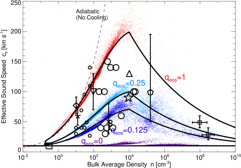
Figure 1 shows the range of effective sound speeds $c_{s}$ in our calculations as a function of the ISM density $n$, compared to a number of observational constraints (large symbols). The solid lines in Figure 1 represent analytic approximations to the equation of state, while the small colored points are representative results from simulations that also include adiabatic cooling/heating and shock heating. We adopt a parameterization of the sound speed as a function of density – i.e. the effective equation of state for the ISM gas – following Springel et al. (2005b); Springel & Hernquist (2005); Robertson et al. (2006a, b). With this model, we can interpolate freely between two extremes using a parameter $q_{\rm eos}$. At one extreme, the gas has an effective sound speed of $10\,{\rm km\,s^{-1}}$, motivated by, e.g., the observed turbulent velocity in atomic gas in nearby spirals or the sound speed of low density photo-ionized gas; this is the “no-feedback” case with $q_{\rm eos}=0$. The opposite extreme, $q_{\rm eos}=1$, represents the “maximal feedback” sub-resolution model of Springel et al. (2005b), based on the multiphase ISM model of McKee & Ostriker (1977); in this case, $100\%$ of the energy from supernovae is assumed to stir up the ISM. This equation of state is substantially stiffer, with effective sound speeds as high as $\sim 200\,{\rm km\,s^{-1}}$. Note that at the highest densities, $c_{s}$ begins to decline in all of the models (albeit slowly), as the efficiency of star formation asymptotes but cooling rates continue to increase.

Varying $q_{\rm eos}$ between these two extremes amounts to varying the effective sound speed of the ISM, with the interpolation

$$c_{s}=\sqrt{q_{\rm eos}\,c_{s}^{2}[q=1]+(1-q_{\rm eos})\,c_{s}^{2}[q=0]}\ .$$ (1)

The resulting sound speeds for $q_{\rm eos}=0.125$ and $0.25$ are shown in Figure 1; these correspond to more moderate values of $c_{s}\sim 30-100\,{\rm km\,s^{-1}}$ for the densities of interest.

Figure 1 compares these models to observations of the turbulent (non-thermal) velocities in atomic and molecular gas in a number of systems (large symbols). At low mean densities, $n\lesssim 0.3-1\,{\rm cm^{-3}}$, the turbulent velocity in nearby spirals is $\sim 10\,{\rm km\,s^{-1}}$. Downes & Solomon (1998) present a detailed study of a number of luminous local starbursts that have significantly higher mean densities; they decompose the observed molecular line profiles into bulk (e.g., rotation) and turbulent motions. We plot their determination of the mean density and turbulent velocities in each system at several radii. We also show the results of similar observations of the core of M82 (Westmoquette et al., 2007), additional nearby luminous infrared galaxies (Bryant & Scoville, 1999), NGC 6240 (Tacconi et al., 1999; Iono et al., 2007), and luminous starbursts at high redshift, $z\sim 2-3$ (Förster Schreiber et al., 2006; Tacconi et al., 2006; Lemoine-Busserolle et al., 2009); at the highest densities, we also show the random velocities observed in the nuclear maser disk in the nearby Seyfert 2 galaxy NGC3079 (Kondratko et al., 2005).

The observational results in Figure 1 favor models with $q_{\rm eos}\approx 0.1-0.3$, albeit with significant scatter. We thus take these values of $q_{\rm eos}$ as our “standard” choices, although we have carried out numerical experiments over the entire range $q_{\rm eos}=0-1$. Note that the observations clearly do not support a simple no-feedback ($q_{\rm eos}=0$) model. Within the range $q_{\rm eos}\approx 0.1-0.3$, our results on AGN fueling are not particularly sensitive to the precise value of $q_{\rm eos}$. Moreover, the functional form $c_{s}(n)$ is also not crucial: simulations using a constant $c_{s}\simeq 50\,{\rm kms^{-1}}$ yield similar results. However, our simulations with $q_{\rm eos}=0$ and $q_{\rm eos}=1$ predict results that are inconsistent with observations of galactic nuclei – thus, our results themselves favor $q_{\rm eos}\approx 0.1-0.3$ (see Appendix B).

For the gas densities of interest in this paper, the precise form of the cooling law does not significantly affect our conclusions. This is because the cooling time is almost always much shorter than the local dynamical time (typical $t_{\rm cool}\sim 10^{-6}-10^{-4}\,t_{\rm dyn}$). As a result the ”sound speed” of the gas is nearly always pinned to the subgrid ‘turbulent’ value discussed above (this is why the numerical points in Fig. 1 are so close to the analytic models). This is true even when the gas is optically thick to the infrared radiation produced by dust, as can readily occur in the central $\sim 100$ pc: the cooling time (diffusion time) is still much less than the dynamical time in the optically thick limit for the radii that we resolve (e.g., Thompson et al. 2005). We have, in fact, experimented with alternative cooling rate prescriptions: including or excluding metal-line cooling, uniformly increasing or decreasing the cooling rate by a factor of $\approx 3$, and in the most extreme case, assuming instantaneous gas cooling (any gas parcel above the cooling floor is assumed to immediately radiate the excess energy in a single timestep). We do not see any significant changes in our results with these variations, simply because the gas always cools rapidly in our calculations (in contrast, in regimes such as the $\alpha$-disk where the cooling time is comparable to the dynamical time, the details of the cooling function can have a significant effect; see Gammie, 2001; Nayakshin et al., 2007; Cossins et al., 2009). If the effective minimum $c_{s}$ comes from turbulent velocities, then the effective cooling time around this oor should be given by the turbulent decay time, which can be comparable to the dynamical time (Begelman & Shlosman, 2009); this is not included in our calculations. In the presence of such an effective cooling time, local gravitational instability may lead to tightly wound spirals as opposed to fragmentation into star-forming clumps. These could be important for angular momentum transport at some radii.

To conclude our discussion of the ISM physics in our simulations, it is important to reiterate that the key role of the sub-resolution sound speed $c_{s}$ is that it determines the local Jeans and Toomre criteria, and thus the physical scale on which gravitational physics dominates. The Jeans mass for a disk of surface density $\Sigma$ and sound speed $c_{s}$ is given by $M_{\rm J}=(\pi\,c_{s}^{4})/(4\,G^{2}\,\Sigma)$. For the outer regions of a galactic disk with $\Sigma\sim 10^{8}-10^{9}\,M_{\sun}\,{\rm kpc^{-2}}$ and $c_{s}\sim 10\,{\rm km\,s^{-1}}$, $M_{J}\sim 10^{6}\,M_{\sun}$, comparable to that of a molecular cloud; the corresponding Jeans length is tens of pc, comparable to that of massive molecular cloud complexes in galaxies. Thus our sub-resolution model is effectively averaging over discrete molecular clouds and star clusters in galaxies. Large-scale inflows can increase the surface density in the central regions of galaxies, but $c_{s}$ also rises. In our models with $q_{\rm eos}\simeq 0.1-0.3$, the Jeans mass remains roughly similar down to $\sim$pc scales, but as a result the Jeans length is significantly smaller in galactic nuclei where the ambient density is much higher. These physical mass and size-scales motivate the numerical resolution in our simulations; in all cases, we ensure that the resolution is sufficient to formally resolve the Jeans mass and length. Higher resolution simulations may be numerically achievable, but can provide only minimal gains in the “reality” of the simulation without a corresponding increase in the sophistication of the ISM model.

2.2 Large Scale Galaxy Mergers and Bars: 100 kpc to 100 pc

Table 1: Galaxy-Scale Simulations 

Simulation $\epsilon$ $q_{\rm eos}$ $f_{\rm gas}$ $h/R$ $B/T(<R)$ $\Sigma_{\rm d}(0)$ $\Sigma_{\rm b}(0)$ $M_{\rm tot}(<R)$ $[M_{\sun}]$ Name [pc] ($500$ pc) ($500$ pc) $(300$ pc) $(1$ kpc) $[M_{\sun}\,{\rm kpc^{-2}}]$ $(300$ pc) $(1$ kpc) (1) (2) (3) (4) (5) (6) (7) (8) (9) Merger & Isolated Galaxy Simulations: Parameter Studies — 20,50,100,150 0.0-1.0 0.05-1.0 0.05-0.35 0.1-0.9 0.01-0.5 1.0e9-1.0e11 1.0e9-1.0e12 1.0e8-1.0e11 1.0e8-1.0e11 Typical Gas-Rich $\sim L_{\ast}$ Merger: Initial Conditions b3ex(ic) 10^a, 50 0.25 0.80 0.25 0.8 0.4 2.5e8 2.5e8 1.4e8 1.9e9 Typical Gas-Rich $\sim L_{\ast}$ Merger: At Coalescence b3ex(co) 10^a, 50 0.25 0.45 0.33 0.15 0.25 2.0e10 2.6e9 4.4e9 2.5e10 Typical Gas-Rich $\sim L_{\ast}$ Merger: $10^{8}$ yr Post-Coalescence b3ex(po) 10^a, 50 0.25 0.08 0.37 0.10 0.15 2.3e11 9.1e9 2.8e10 4.6e10 Bar-Unstable $\sim L_{\ast}$ Disk: Initial Conditions barex(ic) 10^a, 50 0.25 0.40 0.15 0.55 0.35 1.7e8 2.4e8 1.5e8 1.9e9 Bar-Unstable $\sim L_{\ast}$ Disk: At Peak of Inflow barex(pk) 10^a, 50 0.25 0.48 0.20 0.13 0.23 1.1e9 2.5e8 5.2e8 3.8e9 Bar-Unstable $\sim L_{\ast}$ Disk: After Bar Relaxation barex(re) 10^a, 50 0.25 0.04 0.11 0.16 0.18 1.2e10 5.5e9 5.6e9 1.5e10

Parameters describing representative examples of our galaxy-scale simulations of galaxy-galaxy mergers and unstable isolated disks. The top row gives the range spanned in each parameter across our suite of simulations. Subsequent rows pertain to specific examples at chosen times in their evolution. (1) Simulation name/ID. (2) Minimum smoothing length (in pc). (3) Equation of state parameter (Figure 1). (4) Gas fraction $\equiv M_{\rm gas}/(M_{\rm gas}+M_{\ast,\,\rm disk})$ of the disky/cold component (inside the given radius). (5) Scale height of the disky/cold component within the given radius (median $|z|/R$; the plane of the disk is defined by the total angular momentum vector). (6) Bulge-to-total mass ratio inside a given radius (bulge here includes all spherical components: stellar bulge, dark matter halo, and black hole). (7) Maximum surface density of the disky/cold component (gas plus stars) – for an exponential profile, the surface density is nearly constant at radii below the disk scale length. Otherwise, averaged over a couple times our minimum smoothing length. (8) Average surface density inside $300$ pc for the bulge component. (9) Total mass enclosed inside a given radius. All simulations include black holes, but these are dynamically unimportant on these scales.

a

For each of the two simulations here, we have also run three ultra high-resolution simulations which also act as a moderate-resolution intermediate-scale simulations ($\sim 10^{7}$ particles). They are identical in initial conditions to the standard merger and isolated disk run here, with initial gas fraction equal to, one-half, and one-quarter that shown (six simulations in total).

Our galaxy-scale simulations motivate the initial conditions chosen for the smaller-scale re-simulation calculations described in §2.3 & 2.4. The galaxy-scale simulations include isolated disks (both globally stable and bar unstable) and galaxy-galaxy mergers. We will ultimately focus on a few representative examples, but we chose those having surveyed a large parameter space. These simulations and the methodology used for building the initial galaxies are described in more detail in a series of papers (see e.g. Di Matteo et al., 2005; Robertson et al., 2006b; Cox et al., 2006; Younger et al., 2008). We briefly review the key points here.

For each simulation, we generate one or two stable, isolated disk galaxies, each with an extended dark matter halo with a Hernquist (1990) profile, an exponential disk of gas and stars, and an optional stellar bulge. The initial systems are chosen to be consistent with the observed baryonic Tully-Fisher relation and estimated halo-galaxy mass scaling laws (Bell & de Jong, 2001; Kormendy & Freeman, 2004; Mandelbaum et al., 2006, and references therein). The galaxies have total masses $M_{\rm vir}=V_{\rm vir}^{3}/(10GH[z])$ for an initial redshift $z$, with the baryonic disk having a mass fraction $m_{\rm d}$ (typically $m_{\rm d}\simeq 0.041$) relative to the total mass. The system has an initial bulge-to-total baryonic mass ratio $B/T$, and the disk has initial gas fraction $f_{\rm gas}$. The dark matter halos are assigned a concentration parameter scaled as in Robertson et al. (2006b) for the galaxy mass and redshift following Bullock et al. (2001). Disk scale lengths are set in accordance with the above scaling laws.

In previous papers (referenced above), a large suite of these simulations have been presented, with several hundred simulations of varying equation of state, numerical resolution, merger orbital parameters, structural properties (e.g. profile shapes, initial bulge-to-disk ratios, and scale lengths), initial gas fractions, and halo concentrations. In this suite, galaxies have baryonic masses $\sim 10^{8}-10^{13}\,M_{\sun}$ and gas fractions $f_{\rm gas}=0-1$; mergers spanning mass ratios from 1:1 to 1:20, and isolated disks have Toomre Q parameters from $0.1-10$.

In this work, we focus on galaxies with baryonic masses $\sim 10^{11}\,M_{\sun}$. Based on the survey above, we select a representative simulation of a gas-rich major merger and one of an isolated disk, to provide the basis for our subsequent re-simulations. Some of the salient parameters of these simulations are given in Table 1. The merger is equal-mass, with $10^{11}\,M_{\sun}$ galaxies that have gas fractions of $\sim 40\%$ at the time of the merger/coalescence. The orbit is a moderately tilted prograde, parabolic case (orbit e in Cox et al., 2006). Together this makes for a fairly violent, gas rich major merger, representative of many of our other gas-rich major merger simulations at both low and high redshifts. The isolated system is a $10^{11}\,M_{\sun}$ disk with $f_{\rm gas}=0.4$, $B/T=0.3$, scale length $h=3.2\,{\rm kpc}$, and $m_{d}=0.041$; it has a Toomre Q of order one and develops a moderate bar (amplitude $\sim 15\%$), but the gas encounters an inner Linblad resonance at $\sim$1-2 kpc.

Small variations in the orbits or the structural properties of the galaxies will change the details of the tidal and bar features on large scales. However, the precise details of these large-scale simulations are not important for our study of the dynamics on small scales (see Appendix A). Rather, the small-scale dynamics depends on global parameters such as the gas mass channeled into the central region, relative to the pre-existing bulge, disk, and black hole mass. In these respects, we have chosen the simulations summarized in Table 1 to be representative of a broad class of gas-rich systems.

Our galaxy-scale simulations have spatial resolution – gravitational softening length and minimum adaptive SPH smoothing length – of $50\,$pc. In the suite described above, the resolution scales with galaxy mass and is $\sim 50-100\,$pc for $M_{\ast}\sim 10^{11}\,M_{\sun}$ systems, but in a subset of higher-resolution cases is as small as $20\,$pc. In Hopkins et al. (2008b) and Hopkins et al. (2009a) we have demonstrated that this resolution is sufficient to properly resolve not only the mass fractions but also the spatial extent of the “starburst” formed from gas which loses angular momentum in a merger or via a strong bar instability. However, to assess how much of this gas can ultimately fuel a central BH requires that we determine the dynamics on even smaller spatial scales.

2.3 Intermediate Scales: Re-Simulating from 1 kpc to 10 pc

Table 2: Intermediate-Scale Resimulations ($\sim 10-1000$ pc) 

Simulation $\epsilon$ $q_{\rm eos}$ $f_{\rm gas}$ $h/R$ $B/T(<R)$ $\Sigma_{\rm d}(0)$ $\Sigma_{\rm b}(0)$ $M_{\rm tot}(<R)$ $[M_{\sun}]$ Name [pc] ($500$ pc) ($500$ pc) $100$ pc $300$ pc $[M_{\sun}\,{\rm kpc^{-2}}]$ $100$ pc $300$ pc (1) (2) (3) (4) (5) (6) (7) (8) (9) If9b5^a 1.0 0^b,0.175,0.25 0.90 0.30 0.5 0.15 1.0e10 1.1e10 5.4e8 2.9e9 If9b5thin 1.0 0.125,0.25 0.90 0.08,0.16 0.4 0.2 1.0e10 1.1e10 5.4e8 2.9e9 If9b5res 0.3,1,3,10 0.125 0.90 0.30 0.5 0.15 1.0e10 1.1e10 5.4e8 2.9e9 If9b5q 1.0 0,0^c,0.125,0.25,0.5,1 0.90 0.30 0.5 0.15 1.0e10 1.1e10 5.4e8 2.9e9 Ilowresq 3.0 0,0.25,1 0.95 0.27 0.0 0.0 6.0e10 0.0 1.2e9 4.9e9 If1b1late 1.0 0.125 0.096 0.25 0.06 0.03 1.0e11 1.1e10 3.4e9 2.2e10 If1b0late 1.0 0.25 0.091 0.28 0.002 0.003 6.0e10 5.0e8 1.3e9 5.3e9 If1b0lateL^d 2.0 0.25 0.091 0.28 0.005 0.01 6.0e10 5.0e8 7.4e9 8.5e9 If3b3mid 1.0 0.125 0.34 0.25 0.3 0.15 3.1e10 2.0e10 1.3e9 7.2e9 If3b3midRg^e 1.0 0.125 0.45,0.20,0.05 0.3,0.5 0.26 0.12 3.6e10 2.0e10 1.5e9 9.2e9 If1b3Lmid 1.0 0.25 0.10 0.30 0.07 0.10 6.4e10 1.6e9 1.4e9 5.7e9 If1b3LmidL^d 2.0 0.25 0.10 0.30 0.15 0.25 6.4e10 1.6e9 8.4e9 1.1e10 If5b4mbul 1.0 0.25 0.50 0.24 0.40 0.55 7.4e8 1.9e8 0.3e8 1.3e8 If5b8mbul 1.0 0.25 0.50 0.24 0.80 0.90 7.4e8 3.1e9 1.2e8 5.3e8 If9b1lowm 1.0 0.25 0.90 0.15 0.03 0.06 6.4e9 1.2e7 1.3e8 5.4e8 If3b9dsk 1.0 0.25 0.32 0.22 0.95 0.80 1.6e9 1.1e11 2.1e9 6.2e9 If3b9dskL^d 2.0 0.25 0.32 0.22 0.71 0.62 1.6e9 1.1e11 8.0e9 9.3e9 IfXb2gas 1.0 0.25 0.16,0.32,0.50 0.26 0.16 0.08 3.6e10 1.0e10 1.3e9 7.7e9 Inf28b2 1.0 0.20 0.20,0.80 0.25 0.51 0.28 6.3e9 3.0e8 3.6e8 1.7e9 Inf28b4 1.0 0.20 0.20,0.80 0.25 0.67 0.43 3.3e9 3.0e8 2.7e8 1.1e9 Inf28b6 1.0 0.20 0.20,0.80 0.25 0.78 0.56 3.3e9 6.0e8 4.0e8 1.4e9 Inf28b8 1.0 0.20 0.20.0.80 0.25 0.92 0.81 1.0e9 6.0e8 3.4e8 9.5e8 Inf2b9 1.0 0.20 0.20 0.25 0.96 0.89 5.2e8 6.0e8 3.2e8 8.6e8 Inf28b2h^f 0.3 0.125 0.20,0.80 0.25 0.38 0.21 5.5e9 5.0e7 2.3e8 1.1e9 Inf8b2hr^f 0.3 0.20 0.80 0.25 0.17 0.11 5.5e9 2.5e7 2.2e8 1.1e9 Inf28b9h^f 0.3 0.125 0.20,0.80 0.25 0.81 0.75 5.5e9 5.0e10 2.1e9 1.1e10

	Parameters describing our re-simulations of the $0.01-1$ kpc regions from galaxy scale simulations. Parameters separated by commas denote simulations with otherwise identical initial conditions, re-run with the specified parameter varied. (1) Simulation name/ID. (2) Minimum smoothing length (in pc). (3) Equation of state parameter (Figure 1). (4) Initial gas fraction of the disky/cold component (inside the given radius). (5) Initial scale height of the disk component (inside the given radius). (6) Initial bulge-to-total mass ratio inside a given radius (again, bulge refers to all spherical components). (7) Initial maximum surface density of the disky/cold component (gas plus stars). (8) Initial average surface density inside $300$ pc for the bulge component (9) Initial total mass enclosed inside a given radius. All simulations include BHs and dark matter, but these are dynamically unimportant on these scales.
a	A series of 7 runs testing different means of constructing initial conditions, described in Appendix A.
b	Isothermal equation of state, but with a large $c_{s}=50\,{\rm km\,s^{-1}}$ cooling “floor.”
c	Cooling allowed down to $100\,K$, i.e. $c_{s}=1\,{\rm km\,s^{-1}}$.
d	Somewhat larger-scale simulation (between “galaxy scale” and standard “intermediate scale”). Instead of $B/T(<R)$ and $M_{\rm tot}(<R)$ being evaluated at $100$ pc and $300\,$pc, they are here evaluated at $500\,$pc and $1\,$kpc, respectively.
e	Series where the gas disk profile is allowed to vary independent of the stellar disk profile. The gas has exponential, power-law, and truncated power-law profiles, with varying concentrations with respect to the disk (for example including an extended gas “reservoir” at a distance $\sim 2$ times the regular nuclear stellar disk length, with surface density profile $\Sigma\propto R^{-1}$).
f	Very high-resolution simulations which also act as a moderate-resolution nuclear-scale simulations ($2\times 10^{7}$ particles; gas particle mass $\approx 500\,M_{\sun}$). A series of 6 galaxy-scale runs with very high ($\sim 10\,$pc) resolution, used as moderate-resolution intermediate-scale simulations, are also described in the text.

In order to follow the behavior of gas inflow on smaller scales, we re-simulate the central regions of interest at higher resolution, in a series of progressively smaller-scale runs. We begin by selecting a number of representative outputs from the galaxy-scale simulations described above, near the peak of activity. We select several snapshots in the gas-rich merger at key epochs: early close encounters of the two galaxies, just at nuclear coalescence (which is the peak of star formation in the nuclear region), and at the “end” of the merger (roughly $\sim 10^{8}\,$yr after the final coalescence). We also select snapshots typical of isolated, moderately bar-unstable systems, at times where a bar and some inflow has developed; for comparison, we also consider a fully stable (pre-bar) galaxy disk. In each case, we focus on the central $0.1-1$ kpc region, which includes the majority of the gas that has been driven in from larger scales. Some of the representative properties of these snapshots, at these scales and times, are outlined in Table 1.

Our approach to re-simulating the nuclear region is to use the larger-scale simulations to motivate the initial conditions of a smaller scale calculation (a “zoom-in” or “re-simulation”). We do so by de-composing the potential, density, and velocity distributions of the gas, stars, and dark matter at a given time in the larger-scale simulation using the basis expansion proposed in Hernquist & Ostriker (1992). This allows us to not only re-construct a smoothed density profile, but also to include the asymmetric structures from the larger-scale simulation (if desired) and to define where the potential is noise-dominated. From these stellar, gas, and dark matter distributions, we re-populate the gas and stars in the central regions (the scale we wish to re-simulate; generally out to an outer radius of $\sim 1-2\,$kpc) and use this as the initial condition for a new simulation that we run for several local dynamical times. To be conservative, we typically initialize only a small amount of gas in the inner parts of the re-simulation, since the larger-scale simulation from which the initial condition is drawn has little information about the gas properties on small scales; in Appendix  A we show that the subsequent dynamics does not depend significantly on these details of the initial conditions.

We have carried out a total of $\sim 50$ simulations at these intermediate scales, which together span a wide range in the key parameters: the equation of state of the gas and the relative mass fraction in a pre-existing bulge, gas disk, and stellar disk. Table 2 summarizes the key properties of physical importance in several of these simulations (some numerical studies and surveys of initial condition, which turn out to have little effect on the key results, are not listed). Because our general approach is to systematically survey the initial conditions, we do not identify every simulation in Table 2 with an exact snapshot from Table 1; rather, they should be considered a systematic parameter survey of possible intermediate-scale conditions, motivated by the typical range of sub-kpc conditions seen in our galaxy-scale simulations. Dark matter is present, but is dynamically irrelevant at these scales. We have also varied the mass of the central black hole, but at these scales it is still dynamically unimportant. Although the initial conditions for our calculations are drawn from galaxy-scale simulations, the dynamics on small-scales depends primarily on a few key properties of the simulation ($f_{\rm gas}$ and $B/T$), and is thus insensitive to many of the details of the galaxy on larger scales.

Our intermediate scale simulations typically involve $\simeq 10^{6}\,$particles, with a force resolution of a few pc and a particle mass of $\approx 10^{4}\,M_{\sun}$. The duration of the simulation is $\sim 10^{7}-10^{8}\,$yr – this is many dynamical times at small radii, but small compared to the dynamical time at larger radii. These re-simulations can thus be thought of as a probe of the instantaneous behavior of the gas at small radii given the inflow conditions set at larger radii.

We discuss a number of numerical tests and variations about this basic methodology in Appendix A. Specifically, we show that our results are not sensitive to including properties of the larger-scale galaxy in which the simulation should be embedded, such as the $\sim$ kpc-scale tidal potential. They are also not sensitive to whether we initialize an axisymmetric gas/potential distribution, or whether the initial condition includes the non-axisymmetric modes present in the larger-scale simulation. The reason is that instabilities due to self-gravity can grow exponentially from shot-noise in the simulation even given an initially axisymmetric structure. Thus the presence of initial asymmetries on $\sim 100$ pc scales does not have a significant effect on the resulting transport of gas to smaller radii; the transport is determined by the presence (or absence) of internal instabilities in the gas on small scales. Finally, because the “initial” densities on small scales are intentionally initialized to be low relative to their values later in the simulation, our results are not particularly sensitive to how we initialize gas at small radii in the re-simulation; this is important because there is no reliable information about these small-scales in our larger-scale simulation.

To check that our re-simulation approach has not introduced any artificial behavior, we have run a small number of ultra-high resolution galaxy scale simulations, the inner properties of which can be compared to the intermediate scale re-simulations summarized here. For these very high resolution calculations there is continuous inflow from large scales, so they can be self-consistently evolved for many dynamical times. The expense of these calculations, however, limits the survey of initial conditions possible. We have 6 such simulations: three mergers, identical in mass and geometry to our canonical case in Table 1, but with initial $f_{\rm gas}=0.2,\,0.4,\,0.8$, and $\sim 10^{7}$ particles, which gives SPH smoothing lengths of $\sim 10\,$pc. While not quite as high-resolution as our re-simulation runs, these provide an important check on the results of the latter and are run self-consistently for $4\times 10^{9}\,$yr. We will show results from these ultra-high resolution simulations at several points; we find that they are quite similar to our re-simulation runs, thus supporting the methodology used for most of our calculations.

The very high resolution merger calculations also allow us to follow the binary BH pair to much smaller separation (our assumptions lead to rapid merger below $\approx 10\,$pc in these calculations). We confirm, in these cases, that the BH-BH merger precedes most of the gas inflows at $\gtrsim 10$ pc, so that the assumption that the binary has merged is probably reasonable for our re-simulation calculations. Moreover, the gas mass at $\sim 10$ pc is large ($\sim M_{\rm BH}$) in the merger simulations. Thus if gas-rich reservoirs indeed drive rapid BH-BH coalescence, the rapid merger of the two BHs should be a reasonable assumption on all of the scales that we simulate (see e.g. Escala et al., 2004; Perets et al., 2007; Mayer et al., 2007; Perets & Alexander, 2008; Dotti et al., 2009; Cuadra et al., 2009).

2.4 Nuclear Scales: From 10 pc to 0.1 pc

Table 3: Nuclear-Scale Resimulations ($\sim 0.1-100$ pc) 

Simulation $\epsilon$ $q_{\rm eos}$ $f_{\rm gas}$ $h/R$ $M_{\rm BH}$ $M_{\rm b/cl}(<R)$ $\Sigma_{\rm d}(0)$ $M_{\rm d}(<R)$ $[M_{\sun}]$ Name [pc] ($100$ pc) ($100$ pc) $[M_{\sun}]$ $10$ pc $50$ pc $[M_{\sun}\,{\rm kpc^{-2}}]$ $1$ pc $10$ pc $50$ pc (1) (2) (3) (4) (5) (6) (7) (8) (9) Nf8h1c0 0.3 0.0,0.25 0.75 0.16,0.26 2.9e7 1.8e5 3.0e5 7.5e10 1.0e5 1.5e6 1.0e8 Nf8h1c0hol^a 0.3 0.25 0.75 0.24 2.9e7 1.8e5 3.0e5 7.4e10 1.0e3 1.2e6 1.0e8 Nf5h2c1 0.1 0.25 0.50 0.24 3.0e8 1.2e7 8.0e7 1.2e11 3.6e5 2.4e7 1.6e8 Nf28h1c1 0.1 0.25 0.19,0.75 0.27 3.0e7 1.3e7 2.8e7 7.5e10 3.6e5 2.4e7 1.6e8 Nf7h12c0dsk 0.1 0.25 0.70 0.23 2.9e7,3.0e8 0.0 0.0 4.5e9 1.0e4 0.9e6 6.0e6 Nf5h1c0 0.1 0.25 0.48 0.25 2.9e7 0.0 0.0 1.2e11 3.0e5 2.4e7 1.6e8 Nf5h1c2 0.1 0.25 0.48 0.25 2.9e7 3.0e7 9.0e7 1.2e11 3.0e5 2.4e7 1.6e8 Nf8h1c0thin 0.1 0.125 0.75 0.16,0.27 3.0e7 1.8e5 0.3e7 7.6e10 2.0e5 1.5e7 1.0e8 Nf5h1c1thin2 0.1 0.125,0.25 0.50 0.07,0.14 3.0e7 3.0e5 1.2e7 1.2e11 2.0e5 2.4e7 1.6e8 Nf8h1c1qs 0.1 0,0.125,0.25,1 0.75 0.28 3.0e7 3.0e6 1.4e7 7.3e10 2.0e5 1.7e7 1.2e8 Nf8h2c1 0.1 0.25 0.75 0.2,0.33 3.0e8 3.6e6 1.4e7 7.6e10 2.0e5 1.9e7 1.2e8 Nf1h1c1low 0.1 0.25 0.08 0.25 3.0e7 3.5e6 1.4e7 1.7e11 4.7e5 3.7e7 2.5e8 Nf3h1c1mid 0.1 0.20 0.26 0.23 3.0e7 3.5e6 1.4e7 2.1e11 6.0e5 4.6e7 3.0e8 Nf6h12c2dsk 0.1 0.25 0.57 0.22 2.9e7,3.0e8 7.2e6 2.6e7 4.4e9 1.1e5 8.1e6 3.4e7 Nf8h1c3dskM 0.1 0.25 0.75 0.30 2.9e7 1.6e7 7.1e7 7.4e10 3.5e5 3.0e7 1.7e8 Nf8h1c1dens 0.1 0.25 0.75 0.25 3.0e7 3.6e6 1.4e7 3.8e11 1.1e6 8.1e7 5.3e8 Nf8h1c1ICs^b 0.1 0.25 0.75 0.28 3.0e7 3.1e6 1.4e7 7.3e10 2.0e5 1.7e7 1.2e8 Nf8h1c1thin 0.1 0.125,0.18 0.75 0.08,0.17 3.0e7 3.1e6 1.4e7 7.3e10 2.0e5 1.7e7 1.2e8 Nf2h2b2 0.1 0.20 0.20 0.25 3.0e7 6.5e6 2.0e7 3.0e11 8.1e4 7.0e7 4.2e8 Nf8h2b2 0.1 0.20 0.80 0.25 3.0e7 1.3e7 4.0e7 1.5e11 4.7e4 3.5e7 2.1e8 Nf2h2b4 0.1 0.20 0.20 0.25 3.0e7 6.5e6 2.1e7 1.5e11 4.3e4 3.5e7 2.1e8 Nf8h2b4 0.1 0.20 0.80 0.25 3.0e7 1.3e7 4.0e7 7.7e10 2.4e4 1.7e7 1.1e8 Nf2h2b5 0.1 0.20 0.20 0.25 3.0e7 6.5e6 2.1e7 7.7e10 2.1e4 1.8e7 1.1e8 Nf28h2b6 0.1 0.20 0.20,0.80 0.25 3.0e7 1.1e7 3.7e7 3.8e10 1.1e4 8.8e6 5.3e7 Nf8h2b8 0.1 0.20 0.80 0.25 3.0e7 1.3e7 4.1e7 1.5e10 4.7e3 3.5e6 2.1e7 Nf28h2b9 0.1 0.20 0.20,0.80 0.25 3.0e7 1.1e7 3.8e7 9.6e9 2.7e3 2.2e6 1.3e7 Nf8h2b1h 0.015 0.20 0.80 0.25 3.0e7 6.4e6 2.0e7 1.5e11 5.2e4 3.5e7 2.1e8 Nf8h2b3L 0.1 0.20 0.80 0.25 3.0e7 2.3e7 1.1e8 1.5e11 9.3e3 3.9e7 4.9e8 Nf8h2b4q 0.1 0,0.02,0.06,0.12, 0.80 0.25 3.0e7 1.3e7 4.0e7 7.7e10 2.4e4 1.7e7 1.1e8 0.25,0.35,0.5,0.7,1

	Parameters describing our nuclear-scale re-simulations of the sub-$100$ pc regions from intermediate-scale simulations. (1) Simulation name/ID. (2) Minimum smoothing length (in pc). (3) Equation of state parameter (Figure 1). (4) Initial gas fraction of the disky/cold component. (5) Initial scale height of the disky component. (6) Black hole mass ($M_{\sun}$). (7) Initial bulge or nuclear stellar cluster mass, inside the given radius. (8) Initial maximum surface density of the disky/cold component (gas plus stars). (9) Initial mass of the disky component (gas plus stars) inside a given radius (does not include the BH mass or, if significant, nuclear star cluster/bulge mass). Dark matter is insignificant on these scales.
a	Central “hole” is extended in disk out to $5\,$pc.
b	Simulations with no central deficit of matter; the initial density from the larger-scale simulation is extrapolated in to $r\rightarrow 0$. Also expanded into series of initial conditions, as described in Appendix A.

The characteristic initial scale-lengths of the nuclear disks in our intermediate scale calculations are $\sim 0.2-0.5\,$kpc. As we discuss in §3, if the gas fraction is sufficiently large, instabilities quickly develop that transport material down to $\sim 1-10\,$pc, near the resolution limit of our intermediate scale calculations. Material begins to pile up at these radii because the BH mass dominates the potential and the efficiency of large-scale modes decreases at small radii. In order to understand the dynamics on yet smaller scales, we therefore repeat our “re-simulation” methodology once more. The approach is identical to that described above, but this time using the intermediate-scale simulations with resolution of $\lesssim 10\,$pc as our “parent simulation” from which to motivate the initial conditions.

We again carried out $\sim 50\,$ such simulations, typically with $\sim 10^{6}\,$particles, and a force/spatial resolution of $\sim 0.1$ pc (particle mass $\approx 100\,M_{\sun}$). The properties of these simulations are summarized in Table 3. The simulations are evolved for $\sim 10^{5}-10^{6}\,$yr; this is large compared to the dynamical time at the smallest radii $\sim 0.1$ pc, but very small relative to the dynamical time of the larger-scale simulations from which the initial conditions are drawn. The characteristic spatial scale of the re-simulated material is initially $\sim 10-30\,$pc. As described in Appendix  A, we carried out a number of numerical tests of the robustness of these simulations.

At radii $\sim$ pc, the parameters that determine the dynamics are largely the equation of state of the gas, the mass of the BH, the mass of the nuclear disk formed by the inflow from larger scales, and the gas fraction of that nuclear disk. Since the BH dominates the spherical component of the potential at these radii, the “bulge” mass at these radii is only of secondary importance; we include it but find that it makes little difference.

As in §2.3, we have checked the results of these “re-simulations” by carrying out a small subset of ultra-high resolution runs. These extend from $\sim 0.3-1000$ pc and follow inflow from larger scales deep into the potential of the BH; because they resolve larger spatial scales than our typical ”nuclear scale” simulation, these can be run self-consistently for $2\times 10^{8}$ yr. Specifically, we have five such high-resolution intermediate scale simulations (see Table 2), three with initial $f_{\rm gas}=0.8$ (a low, intermediate, and high $B/T$ case), and two with $f_{\rm gas}=0.2$ (low and high $B/T$). They have $\sim 10^{7}$ particles and gravitational softening lengths of $\sim 0.3\,$pc. We show the results from these runs explicitly at several points; we find that they are completely consistent with our survey of re-simulations, which cover a larger parameter space of galaxy/BH properties, but are more limited in dynamic range.

It is important to note up-front that our simplified treatment of the ISM physics becomes particularly suspect on nuclear scales $\sim$ pc. At these radii, our assumption that we can average over the dynamics of stellar winds, supernovae, HII regions, etc. and define an effective ISM equation of state may break down. Nonetheless, we believe that the efficient angular momentum transport found here is likely generic, so long as some of the gas is prevented from forming stars and the gas fraction is sufficiently high that instabilities generated by self-gravity are initiated. The fact that the main sequence lifetime of a massive star is longer than the local dynamical time on small scales probably increases the efficacy of stellar feedback and decreases the fraction of the gas turned into stars per dynamical time (Murray et al., 2009).

At scales $\ll 0.1\,$pc, the potential is fully Keplerian and viscous heating is sufficient to stabilize the disk against its own self-gravity (i.e., $Q\gtrsim 1$) (Goodman, 2003). At these radii, the system begins to approach a traditional accretion disk. Given the cessation of star formation and the deep potential well of the BH, we assume that the inflow rate at $\sim 0.1$ pc is a reasonable proxy for the true accretion rate onto the BH. Because our simulations are not well-suited to describe the physics of the disk on scales $\lesssim 0.1$ pc, we do not perform a further “zoom in.”

3 Overview: From kpc to sub-pc Scales

Figure 2: Example of our multi-scale simulations used to follow gas flows from $\sim 100\,$kpc to $\sim 0.1\,$pc. Each row is a separate simulation, with the initial conditions for the intermediate and nuclear-scale simulations taken from the output of the larger-scale runs in the row above it. Each panel shows the projected gas density (intensity) and effective sound speed (color; blue is gas with an effective $c_{s}\sim 10\,{\rm km\,s^{-1}}$, through yellow at $\sim 100-200\,{\rm km\,s^{-1}}$). Each image is rotated to project the gas density “face on” relative to its angular momentum vector. From top left to bottom right, panels zoom in to the nuclear region around the BH, with resolution spanning a factor $\sim 10^{6}$ in radius. Top: Large-scale gas-rich galaxy-galaxy major merger simulation, just after the coalescence of the two nuclei (run b3ex(co) in Table 1). The apparent second nucleus is actually a clump formed from gravitational instability. Middle: A higher-resolution re-simulation of the conditions in the central kpc (run If3b3midRg in Table 2). Despite the fact that the background potential is largely relaxed on these scales, the very large gas inflows lead to a strongly self-gravitating disk on $\sim 0.5\,$kpc scales that develops a strong spiral instability, leading to efficient angular momentum transport to $\sim 10\,$pc. Again, some clumping appears (there is only one nucleus). Bottom: High resolution re-simulation of the central $\sim 30$ pc of the intermediate-scale simulation, with a resolution $\sim 0.1\,$pc (run Nf5h1c2 in Table 3). The potential is quasi-Keplerian, suppressing traditional bar and spiral instabilities, but the large inflows lead to a self-gravitating system that develops a standing eccentric disk mode (single-armed $m=1$). The stellar and gaseous eccentric disks precess relative to one another on $\sim 1-10\,$pc scales and drive efficient inflows of $\sim 10\,M_{\sun}\,{\rm yr^{-1}}$ into the central $0.1\,$pc.

Using the numerical simulations described in §2, we now describe how gas is transported from $\gg$kpc scales to $\ll$pc scales. Initially, our discussion is somewhat qualitative; we focus on emphasizing the key physics at play and our key results. In § 5 we discuss the relevant stability criteria more quantitatively, and outline some specific criteria necessary for “interesting” gas inflow.

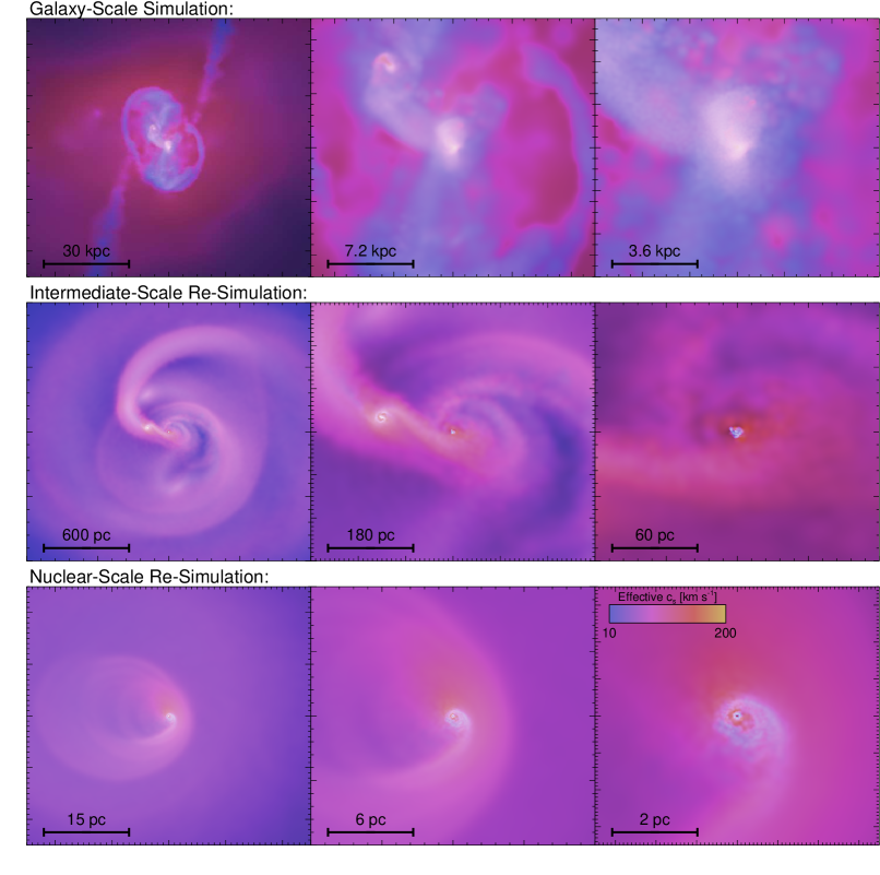
Figure 2 shows an illustrative example of the results of our re-simulations on various scales. We plot gas surface density maps, with color encoding the gas effective sound speed, from scales of $\sim 100\,$kpc to $<1\,$pc. The simulation in this case is a fairly gas-rich major merger ($f_{\rm gas}\sim 30-40\%$ at the time of the final coalescence) of two $5\times 10^{10}\,M_{\sun}$ baryonic mass galaxies. The smaller scale re-simulations were carried out just after the coalescence of the two nuclei, which is near the peak of star formation activity, but when the system is still quite gas rich. The initial systems had pre-existing bulges of $\sim 1/3$ the disk mass and BHs initialized on the $M_{\rm BH}-\sigma$ relation ($\sim 10^{7}\,M_{\sun}$). Each panel is rotated so that the view is close to “face-on” with respect to the total angular momentum vector of the gas plotted in the image. Viewed edge-on, much of the gas forms a modestly thin ($H/R\lesssim 0.3$) disky distribution at all radii.

3.1 Large Scales: Mergers and Bars

From $\sim 100\,$kpc to $\gtrsim 100\,$pc, the gas flows are well-resolved by our galaxy-scale simulation. In mergers, the final collision of the two galaxies yields strong torques that efficiently cause most of the gas to flow to the center on a timescale approximately equal to a few dynamical times. This process has been described in detail in e.g. Hopkins et al. (2009b), and references therein, but for completeness we briefly summarize the important physics. The secondary/merging galaxy does not directly torque the gas. Rather, the torques on the gas are dominated by local torques from stars originally in the same disk as the gas. The merger induces triaxial “sloshes” and bar-like structures in the stars, i.e., non-axisymmetric modes, supported by radial and/or random orbits. These are also induced in the gas. However, because the gas is dissipational, the gaseous modes slightly lead those in the stars. The stellar disturbance, being physically close to, trailing, and in near-resonance with the gas, produces a strong torque that removes angular momentum from the gas and easily dominates the total torque (torques directly from the secondary galaxy, from the primary halo, or hydrodynamic torques from shocks or internal clump collisions, are all $\lesssim 10\%$ effects; see e.g. Barnes & Hernquist, 1996; Barnes, 1998; Hopkins et al., 2009b).

Figure 3: Images of the morphologies of the secondary instabilities that develop on intermediate scales ($\sim 100$ pc), as a consequence of galactic-scale torques bringing gas into the central kpc. Each panel shows projected gas density (intensity) and local star formation rate (color, from blue through yellow) in the central kpc. We sort the simulations by the parameters that have the largest impact on the dynamics: the bulge-to-disk ratio (disk being both stellar and gaseous) within $300\,$pc and gas fraction $M_{\rm gas}/(M_{\rm gas}+M_{\ast,\ \rm disk})$: from top – bulge-dominated systems with $B/T\gtrsim 0.8$ to bottom – disk-dominated systems with $B/T\lesssim 0.1,$ and from left – systems with $f_{\rm gas}\lesssim 0.1$ to right – systems with $f_{\rm gas}\gtrsim 0.8$. Global instabilities become more prominent with decreasing $B/T$; local instabilities (clumping/fragmentation and/or more tightly wound spirals) become more prominent with increasing $f_{\rm gas}$. The simulations at fixed B/T and/or $f_{\rm gas}$ are similar, but include variation in e.g. the initial mass profile shapes; this contributes to the dramatic diversity of morphologies on nuclear scales. Almost all systems that are not entirely bulge-dominated develop strong large-scale instabilities that efficiently transport gas to $\sim 10\,$pc. Observationally, these would be categorized as a mix of bars, spirals, nuclear rings, crossed rings, fragmentation/clump instabilities, and single or triple-armed spirals.

After the two galactic nuclei coalesce, the disturbances in the stellar component of the galaxy relax away in a number of crossing times. Until they relax, gas inflows continue. Moreover, the coalescence of the nuclei completes much more rapidly, in a timescale close to a single crossing time, at least in a major merger. Thus, a significant fraction of the gas inflows can occur in the background of a rapidly relaxing stellar potential, in the wake of the nuclear coalescence. This is the stage illustrated in Figure 2.

The gas that loses angular momentum flows in to radii $\sim 0.5-1\,$kpc (for an $\sim L_{\ast}$ system), where it participates in a nuclear starburst and builds a dense central stellar mass concentration, critical for establishing the structural properties and size of the remnant spheroid. At these scales, the system is often gas-dominated for a short period of time owing to these inflows (provided the merger is sufficiently gas-rich). However, as the gas forms stars, the central region will quickly become more stellar-dominated; because these stars form out of the gaseous disk, in the relaxing potential — they are not themselves violently relaxed. This is important for the subsequent evolution of the system because of the presence of disk instabilities that would be suppressed by a larger dispersion-supported (spherical) component in the very central region.

The general scenario summarized here can be applied not just to major mergers, but also to minor mergers, fly-by encounters, and even sufficiently bar-unstable stellar disks. The details will be different, but the qualitative steps above, and the exchange of angular momentum between gas and stars, is robust, ultimately leading to inflow to sub-kpc scales. The subsequent evolution depends largely how much material is efficiently channeled to small radii (relative to the bulge and BH mass), not on how that material gets there.

3.2 Morphology and Gas Transport From 1 kpc to 10 pc

3.2.1 General Behavior

The gas infalling from large radii begins to “pile up” at radii $\sim 0.1-1$ kpc, rather than continuously flowing in to yet smaller radii. This is because the torques from the disturbances at large radii become less efficient at small radii. This happens for three reasons: (1) In the merger context, the stellar perturbation at small radii relaxes after coalescence, decreasing the efficiency of gas inflow. (2) The rapid gas inflow implies that the system becomes increasingly gas-dominated at radii $\sim 100$ pc, even if the initial disk gas fraction is low, $\sim 0.1$. Because the primary angular momentum sink of the gas is the local stars, when the system becomes locally gas-dominated, angular momentum transfer is actually less efficient (see Hopkins et al., 2009b, f). (3) The gas can encounter the equivalent of an inner Linblad resonance. This is especially important for unstable gas bars, minor mergers, and disturbances induced by early passages. For the case of coalescence following major mergers, the disturbance is not a single mode, but a series of modes at all scales. As such, there is often no formal inner Linblad resonance or angular momentum barrier (each mode may have such a barrier, but these are spread over a wide range of scales; there is thus a means to overcome the barrier associated with any single mode).

Figure 2 shows the outcome of gas pile-up in the central kpc using an intermediate-scale re-simulation (middle row). In this case, the intermediate scale simulation is a high-resolution re-simulation of the larger-scale gas distribution at a given epoch in a gas-rich major merger. The gas density reached from the larger-scale inflows is quite large – $\sim 10^{10}\,M_{\sun}$ worth of gas has formed a disky component with a scale length of $0.3\,$kpc and an average surface density of $\sim 10^{10}\,M_{\sun}\,{\rm kpc^{-2}}$. This is a large fraction of the galaxy mass – larger than the pre-existing bulge within these radii. The small-scale gas disk is therefore strongly self-gravitating. Indeed, we see from Figure 2 that it quickly develops unstable, non-axisymmetric modes. This is essentially the “bars within bars” scenario predicted by Shlosman et al. (1989), although the morphology of the system is clearly not a simple bar; this is an important point to which we return below. The strength of the modes that develop in this re-simulation depend on the fact that there is star formation in the gas – as the gas turns into stars in situ, those stars develop non-axisymmetric modes, and the two precess relative to one another. As in the galactic-scale torques discussed above, this produces particularly efficient angular momentum transport. These processes ultimately lead to a significant amount of gas flowing down to $\sim 10\,$pc.

3.2.2 Diversity in Morphologies and Inflow Strengths

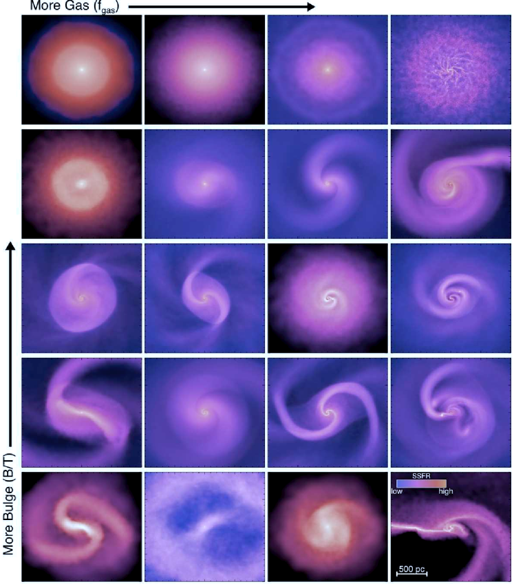
For our fiducial parameterization of the ISM equation of state, the disk-to-bulge ratio and gas fraction on $\simeq 0.1-0.3$ kpc scales have the largest influence on the dynamics and angular momentum transport in our intermediate-scale simulations (for discussion of the role of $q_{\rm EOS}$ and sub-resolution physics, see Appendix B). Figure 3 illustrates this by showing the $\sim 100$ pc scale morphology of a representative subset of our intermediate scale re-simulations, each after a couple of local dynamical times of evolution ($\sim 10^{7}-10^{8}\,$yr). These are sorted by gas fraction $f_{g}$ and $B/T$.

As Figure 3 shows, systems with very large $B/T\gtrsim 0.9$ (top row) are globally stable, as expected analytically. In the extremely gas-rich, large $B/T$, case (top right), local Toomre-scale instabilities develop – if such small clumps were infinitely long-lived, their orbits would decay via dynamical friction and allow for some transport of gas to the center. However, because the clumps are dense, they quickly turn into stars – such a mechanism is largely a means to move stars to the galactic nucleus, not gas (and in fact leads to nuclear stellar clusters much larger than those observed; see Appendix B for a more detailed discussion). Previous claims that such clump-sinking could efficiently fuel BH growth (see e.g. the discussion in Wada et al., 2009; Kawakatu & Wada, 2008, and references therein) have neglected star formation and have thus dramatically over-estimated the inflow of gas via this process. Local clumping instabilities like these do, of course, occur, forming molecular clouds and star clusters. However, there are both theoretical and observational arguments that suggest that they quickly dissolve on a few local dynamical times, probably via feedback from some combination of stellar winds, HII regions, and radiation pressure (Larson, 1981; Blitz, 1993; Krumholz et al., 2006; Allen et al., 2007; Bonnell et al., 2006; Elmegreen, 2007). We also note that, under certain conditions, such local instabilities could instead produce small scale, tightly wound spiral waves instead of leading to fragmentation (e.g. Lodato & Rice, 2004; Rice et al., 2005; Boley et al., 2006); however, this generally occurs when the cooling time is comparable to or larger than the dynamical time, which is not the case in these simulations (although it will also depend on the turbulent decay time which, if sufficiently large, can allow turbulence to suppress runaway clumping and star formation).

Figure 4: Images of the instabilities that develop in our small-scale ($\sim 10$ pc) nuclear re-simulations with $0.1\,$pc resolution. Each panel shows projected gas density (intensity) and local star formation rate (color, from blue through yellow) in the central kpc. Each of these simulations can be thought of as a simulation of the corresponding nuclear scales from Figure 3. The simulations extend into the BH radius of influence. The primary parameters of importance are the ratio of the gas mass to the BH mass (or BH plus bulge/star cluster mass, when the latter is present) and the gas fraction in the disky component: top to bottom is decreasing BH/stellar mass while the disk gas fraction increases from left to right. A strong $m=1$ mode is generic for reasonable BH/stellar mass and gas fractions – this corresponds to an eccentric, globally precessing (non-winding) disk (or single-armed spiral), a mode that is special to the quasi-Keplerian potential. The resulting torques drive inflows of up to $10\,M_{\sun}\,{\rm yr^{-1}}$ at $<0.1\,$pc scales (Figure 5), sufficient to fuel a luminous quasar.

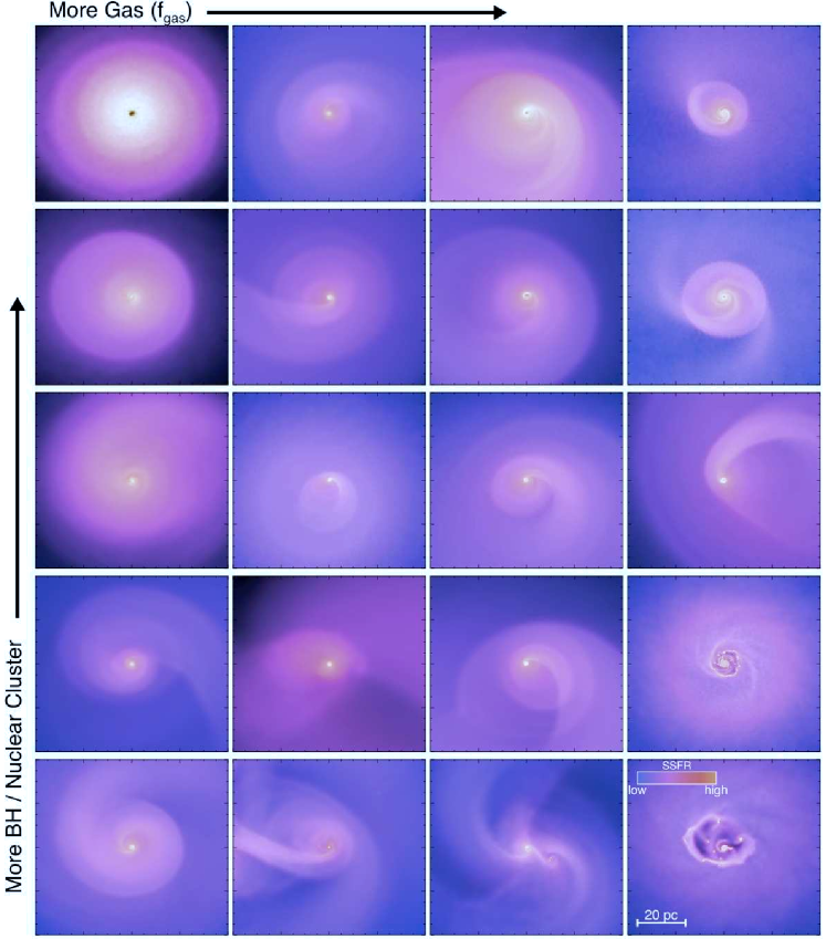
Figure 3 demonstrates that the strength of global non-axisymmetric modes increases dramatically with decreasing $B/T$. In fact, as soon as the bulge and disk are comparable (second row from top), prominent modes appear. In the disk-dominated cases (bottom row), very large angular momentum transport occurs even in cases without much total gas. Of course, at each $B/T$, increasing the gas content makes the system more vulnerable to local instabilities as well – usually making the overall inflow more clumpy and time-variable. In several cases, the large-scale mode (e.g. a spiral arm) becomes self-gravitating and globally fragments (not necessarily into smaller sub-units, but as a whole), leading to a major coalescence – what is almost (dynamically speaking) a scaled-down merger in the central regions!

Figure 3 also demonstrates an important point seen in Figure 2. Although the instabilities seen in our simulations qualitatively resemble the “bars within bars” idea of secondary instabilities once the gas density is sufficiently high, the morphologies vary widely, and are not restricted to traditional bars (although these certainly do appear). At similar gas fraction and $B/T$, we find that the strength of angular momentum transfer is generally similar, but we also find that the visual morphology (and the precise modes important for transport) can vary widely, depending on time and on the details of the gas, stellar disk, bulge, and halo profiles, and the precise equation of state. Thus, global quantities such as the mass profile and accretion rate are comparatively robust, but the observational classification of these systems would vary widely. Indeed, Figure 3 shows traditional bars and spirals, nuclear rings, crossed or barred rings, single or three-armed systems, flocculent disks, and clumpy, irregular morphologies. These all appear, with no obvious preference for one or another as a whole, in our simulations.

This feature of our simulations may account for a number of observational results in the literature. For example, surveys of AGN have often found that although nuclear bars on these scales only appear in some fraction of sources (not necessarily much larger than the fraction of non-AGN in which they appear), there are ubiquitous asymmetric gas structures of some sort, similar to those modeled here (see e.g. Martini & Pogge, 1999; García-Burillo et al., 2005; Haan et al., 2009; Krips et al., 2007; Laine et al., 2002; Peletier et al., 1999; Sakamoto et al., 1999). We discuss this further in § 7.

3.3 Towards the Accretion Disk: Eccentric Disks at $\sim$ Parsec

From $\sim 500$ to $\sim 10\,$pc, our intermediate-scale simulations successfully demonstrate efficient angular momentum transport via a wide range of gravitationally unstable modes. Near the smallest radii in these simulations, however, the systems encounter yet another angular momentum barrier. At that point, gas has reached the BH radius of influence, i.e., the BH begins to contribute non-trivially to the potential, which becomes quasi-Keplerian. This halts further inflow because the disk is no longer strongly self-gravitating and so is less susceptible to global modes. In addition, the gas generally encounters an inner Linblad resonance associated with the intermediate-scale bar.

Indeed, it is widely appreciated that both “bars within bars” and the direct or induced torques due to perturbations from mergers, close passages, and large-scale bars do not produce efficient angular momentum transfer at radii $\sim 0.1-10\,$pc (see e.g. the discussion in Athanassoula et al., 1983, 2005; Shlosman et al., 1989; Heller et al., 2001; Begelman & Shlosman, 2009, and references therein). As a consequence this is often considered the most difficult-to-explain regime of gas inflow and angular momentum transport.

Figure 5: Time-dependent inflow rate through various radii, for the example simulation shown in Figure 2. Main: Gas inflow rate into the central $300\,$pc in the large-scale galaxy merger simulation, as a function of time since the beginning of the merger. The large spike follows the coalescence of the two nuclei. Dotted line shows the instantaneous inflow rates; solid line shows the inflow rate averaged over five local dynamical times. Top Right: Inflow rates into the central $\sim 10$ pc in the intermediate scale re-simulation for a small time interval just after coalescence. Top Left: Inflow rates into $0.1$ pc in our smallest-scale resimulation, initialized with conditions from the previous intermediate-scale simulation after it has evolved for several local dynamical times. The accretion rate reaches $1-10M_{\odot}\,{\rm yr^{-1}}$, sufficient to fuel a luminous quasar. Note the episodic, highly variable nature of accretion/inflow at each scale.

We find, however, that efficient angular momentum transfer continues in our smaller-scale re-simulations for sufficiently gas-rich, disk-dominated systems. Figure 4 shows this with images spanning a range of $f_{g}$ and $B/T$; we will discuss this physics in more detail in §4 & 5. These results show that, so long as the gas density is sufficiently large (relative to the BH mass), the system develops a precessing eccentric disk (an $m=1$ mode) that drives gas down to sub-pc scales $\sim 0.1$ pc. As before, stars rapidly form out of the disk, leading to a similar mode in both the stars and gas; these modes precess about the BH relative to one another with slightly different pattern speeds, leading to crossing orbits, dissipation of energy and angular momentum in the gas, and thus net inflow. This is, once again, an instability that depends primarily on the presence of sufficient gas at small radii in the first place. We find that this condition is met at some point(s) in time in all of our simulations with significant gas mass and instability at $\sim 100\,$pc, i.e., in those simulations that meet the “bars within bars” criteria in §3.2 and Figure 3.

4 Inflow Rates and Gas Properties

Figure 6: Time-dependent inflow rate through various radii, as in Figure 5, but for a simulation in which the large-scale inflow into the central kpc is weak (simulation barex in Table 1). Specifically, this is a gas-rich disk with $B/T=0.3$, which is moderately bar-unstable. Compared to a major merger, the inflow to $<300$ pc is much weaker, and the presence of an inner Linblad resonance at small radii leads to both outflow and inflow from the bar. Because of the much lower gas supply to the inner part of the galaxy, secondary instabilities do not efficiently develop that can transport gas further in.

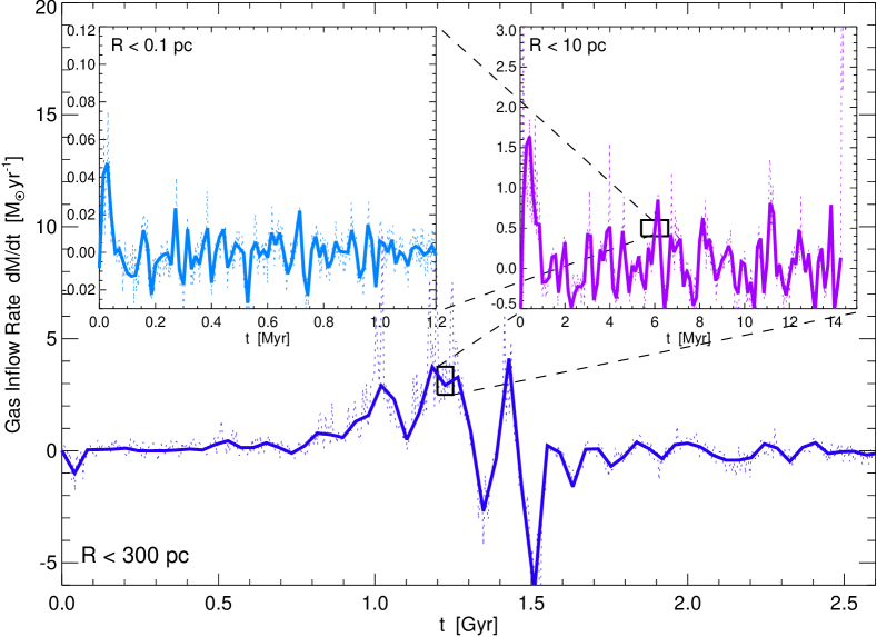
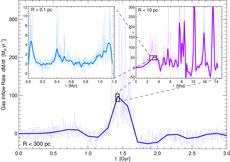
Figure 5 shows the time-dependent inflow rates through several annuli, for the same set of multi-scale re-simulations shown in Figure 2. These demonstrate and quantify the general scenario summarized above: on large scales, coalescence and the final stages of the merger drive a large quantity of gas into the central few hundred pc, with inflow rates $\sim 100-300\,M_{\sun}\,{\rm yr^{-1}}$. The total duration of this phase is a few times $10^{8}$ yr. During this time, the gas accumulates at small radii $\sim 100$ pc; simulating the dynamics on this scale for $\sim 10^{7}\,$yr, we find that secondary gravitational instabilities develop that drive further inflows into the central $\sim 10\,$pc, with inflow rates $\sim 10-200\,M_{\sun}\,{\rm yr^{-1}}$. Zooming in yet again during one epoch of significant inflow to $\lesssim 10$ pc, our smallest-scale simulations resolve the rapid formation of an eccentric nuclear disk around the central BH; the accretion rate into the central $0.1$ pc, which is likely a reasonable proxy for the accretion rate onto the BH, reaches $\sim 1-10\,M_{\sun}\,{\rm yr^{-1}}$. This is sufficient to fuel a luminous AGN at the Eddington rate.

Figure 5 also demonstrates that the small-scale accretion rate can be highly time-variable. This is in part a consequence of the accretion of individual clumps/clouds (e.g., Fig. 4), but is also a consequence of the fact that gravitationally unstable perturbations rapidly grow, dissipate, and generate other structures; depending on, e.g., the state of precession of the stellar versus gaseous disk, the system can transition between inflow and outflow at a given radius. Even on the largest scales, the inflow is still highly variable, although is coherent over a time much longer than the dynamical time because it is driven by the global torques involved in the merger. Because of the variability in $\dot{M}$ on different scales, we do not expect every merger (or isolated galaxy with a large-scale bar), at every time, to exhibit significant inflow from large scales all the way down to the BH. This is important – after all, a large fraction of observed mergers are not bright quasars. In addition, the large variation in the physical conditions at small radii for a relatively fixed set of conditions at larger radii demonstrates that great care must be taken when trying to correlate the galactic structure at $\sim 0.1-1$ kpc with the BH accretion rate in order to constrain the physics of AGN fueling.

Figure 6 shows the same calculation of the inflow rates, but for re-simulations of an isolated disk galaxy with a moderate bar instability (the case in Table 1). The system develops a fairly strong bar at about a kpc (representing a perturbation to the potential of $\delta\Phi/\Phi\sim 0.15$), but this is still much weaker than the major merger case shown in Fig 5; moreover, the pre-existing bulge with $B/T=0.3$ means that there is an inner Linblad resonance at a few hundred pc. The net result is that the overall inflow is much weaker, and there can be outflow as well as inflow on small scales (the system overcomes the Lindblad resonance for short periods of time, leading to inflow followed by outflow as it re-equilibrates). Re-simulating smaller scales, the weak inflows produced by the bar lead to low gas mass ($\sim 1-10\%$) relative to the bulge mass on small scales, and global secondary instabilities do not develop. Inflow/outflow rates from the bar at $0.3-1\,$kpc are characteristically $\sim 0.5-10\,M_{\sun}\,{\rm yr^{-1}}$, similar to observed local barred galaxies (Quillen et al., 1995; Jogee et al., 2005; Haan et al., 2009); at $\sim 10\,$pc they do not exceed $1\,M_{\sun}\,{\rm yr^{-1}}$, and at $<0.1\,$pc they are characteristically $\ll 0.1\,M_{\sun}\,{\rm yr^{-1}}$. At these low accretion rates our calculations are not reliable, but the key point is that in the low gas fraction limit, gravitational torques drive very little accretion from $\sim$ kpc to $\lesssim 0.1$ pc, even in the presence of a modest bar at $\sim$ kpc.

Figure 7: Radial profile of the specific torque in a representative nuclear scale simulation (Nf8h1c1qs in Table 3) during a stage of rapid BH accretion. The torque per unit mass acting on the gas is averaged over narrow radial annuli at one time; negative torques decrease the gas angular momentum. The total gravitational torque (black line) is divided into the torque from stars in the same disk as the gas (purple), gas (red), and the contribution from the large-scale tidal field (orange). The hydrodynamic torques from pressure forces and artificial viscosity (green) are comparatively small. Inflow at all radii is dominated by gravitational torques, largely from nearby stars in the same $m=1$ pattern as the gas.

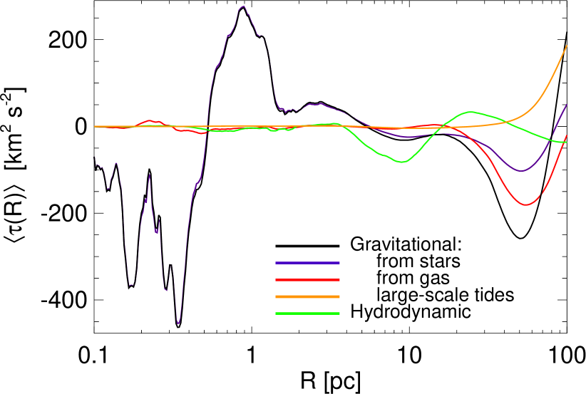
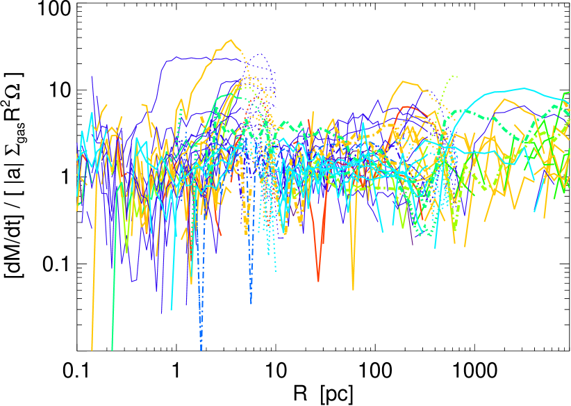
Figure 7 shows an example of the torques driving the inflows in our high accretion rate simulations. We show the radial torque profile at one time in one of our nuclear-scale simulations, broken down into gravitational torques from the stars and gas in the nuclear disk (versus the large-scale tidal field) and hydrodynamic torques (largely from pressure forces); note that negative torques drive inflow. The average gravitational torque in an annulus between $R_{0}$ and $R_{0}+\Delta R$, from sources $j$, is defined by

$${\bf\tau}_{\rm grav,\,j} \equiv\frac{1}{M_{\rm gas}[\Delta R]}\int_{R_{0}}^{R_{0}+\Delta R}\,\rho_{\rm gas}({\bf r})\,{[}{\bf r}\times{\bf a_{\rm grav,\,j}}{]}_{z}\,{\rm d}r\,{\rm d}\cos{\theta}\,{\rm d}\phi$$

$$=\frac{1}{M_{\rm gas}[\Delta R]}\,\sum_{i\ {\rm in}\ \Delta R}m_{i}\,{[}{\bf{r}_{i}}\times\nabla\Phi_{j}({\bf r_{i}}){]_{z}}$$ (2)

where $M_{\rm gas}[\Delta R]=\sum m_{i}$ is the gas mass in the annulus; the sum over $i$ in the second expression refers to the gas particles inside the annulus, while $\Phi_{j}$ is the gravitational potential generated by the torquing particles of interest (gas, stars, etc.). The radius ${\bf r}$ is defined with respect to the BH, and we focus on the $z$ component of ${\bf\tau}$, where the $z$ axis is defined to be the angular momentum vector of the disk (torques in the other directions are negligible, so this is almost identical to plotting $|{\bf\tau}|$). The torques from pressure forces are similarly defined by

$${\bf\tau}_{\rm P,\,j} \equiv\frac{1}{M_{\rm gas}[\Delta R]}\int_{R_{0}}^{R_{0}+\Delta R}\,\rho_{\rm gas}({\bf r})\,{[}{\bf r}\times{\bf a_{\rm P}}{]}_{z}\,{\rm d}r\,{\rm d}\cos{\theta}\,{\rm d}\phi$$

$$=\frac{1}{M_{\rm gas}[\Delta R]}\,\sum_{i\ {\rm in}\ \Delta R}m_{i}\,{[}{\bf{r}_{i}}\times\frac{1}{\rho({\bf r_{i}})}\nabla P({\bf r_{i}}){]_{z}}$$ (3)

where the pressures and densities are determined in standard fashion from the SPH quantities. Note that the BH can and does move (with typical amplitude $R\sim 0.1\,R[M_{d}(<R)\sim 0.1\,M_{\rm BH}]$) in response to the $m=1$ modes on nuclear scales; but since we are interested in the inflow onto the BH itself, we evaluate these torques about its instantaneous position (rather than, say, the center-of-mass of the system). The results are qualitatively similar in Figure 7 if we fix the central position (albeit quantitatively altered within $\ll 10\,$pc at a factor $\sim 2$ level), but are less directly relevant to interpreting inflow onto the BH.

The qualitative behavior shown in Figure 7 is representative of all of our simulations. At essentially all radii, gravitational torques dominate hydrodynamic torques. Moreover, the gravitational torques themselves are dominated by torques from stars, not the torques of the gas on itself; specifically, the stars that are important are in the same asymmetric perturbation as the gas. This is also the case on larger scales ($\gtrsim 100\,$pc), for both mergers and barred systems (see Barnes & Hernquist, 1996; Hopkins et al., 2009b). Torques from the spherical component of the system (e.g. the halo and/or bulge stars) are negligible at all radii. Unsurprisingly, the torques from the large-scale tidal field, defined here as the torques from the $\gg 100\,$pc scales of the parent simulation from which the initial conditions of this re-simulation were drawn, become significant only at the outer boundary of our re-simulation (see Appendix  A.2). Figure 7 shows that there are several sign changes in the torque profile, reflecting the specific state of the system at this time; the torque is time variable, but we find there are sign changes as well in a time-averaged sense. Overall, the net rate of change of the angular momentum of the gas very closely tracks the time-averaged gravitational torque from the stars. Hydrodynamic torques never induce very strong torques (greater than those shown), whereas the stellar gravitational torques can be a factor of $\sim 10-100$ larger than in Figure 7 at some times.

Figure 8: Properties of representative galactic (right panel), intermediate (middle), and nuclear-scale (left) simulations as a function of radius at a single time. The simulations are the same as in Figures 2 & 5 and the time chosen corresponds to near the peak of activity, with significant gas inflow to small radii. Note that the initial/boundary conditions for the smaller-scale simulations were taken from the larger-scale simulations shown, so the results are reasonably continuous at the radial boundaries (despite the fact that these do not represent a self-consistent single simulation). Top: Gas and stellar surface density. Second-from-Top: Enclosed star formation rate in a given radius. Middle: Instantaneous inflow/outflow rate through the annulus (black line); note that there are several sign changes as a function of radius. Also shown is the order of magnitude estimate of the accretion rate produced by gravitational torques from a non-axisymmetric mode of amplitude $|a|$, $\dot{M}\sim|a|\,\Sigma_{\rm gas}\,R^{2}\,\Omega$ (dashed red line; § 4). Second-from-Bottom: Scale height $z_{0}/R$ of the gas. Bottom: Toomre $Q$ parameter of the gas.

The fact that the torques on the gas are dominated by stars is robust, and occurs for two reasons. First, the stars contribute significantly to the mass on the scales $\gtrsim 0.1$ pc that we focus on here (where star formation can occur). For typical star formation efficiencies, it is difficult to have the gas mass $\gg 50\%$ of the total mass for a reasonable fraction of the lifetime of the system. On large scales, galaxies are known to not be so gas rich (although they certainly can reach $\sim 50\%$ gas fraction). On small scales, if the star formation efficiency is a few percent per dynamical time, then even a pure gas inflow from larger scales is likely to only remain gas-dominated for $\sim 10$ local dynamical times (on the smallest scales, $\sim 10^{6}\,$yr) – thus for the majority of the time during which inflow is continued, the system will contain a significant stellar mass. This is consistent with direct observations of sub-kpc regions of starburst galaxies (Downes & Solomon, 1998; Bryant & Scoville, 1999) and the $\sim 1-10$ pc nuclear scales around AGN (Hicks et al., 2009). On sufficiently small scales, $\lesssim 0.01-0.1$ pc, star formation will become inefficient, but at precisely those radii, we have (by definition) essentially reached the $\alpha$-disk.

Figure 9: Comparison of the true instantaneous inflow rate in the simulations (${\rm d}M/{\rm d}t$) to the simple dimensional scaling $|a|\,\Sigma_{\rm gas}\,R^{2}\,\Omega(R)$ expected for pure gravitational torques, where $|a|$ is the magnitude of the strongest non-axisymmetric mode at a given radius $R$ (directly measured in the simulations; with typical values $\sim 0.01-0.3$). Each solid line denotes a different simulation, with dotted lines showing the radii near the boundaries of our re-simulations, where the exact profile shape is suspect; colors correspond to initial gas fractions as in Figure 13. Thick dot-dashed lines correspond to ultra-high resolution simulations. The simulations are shown during the active/strong inflow phases, as in Figure 5. The inflow rate in the simulations is consistent with being produced by gravitational torques over $5$ orders of magnitude in radius, with relatively little scatter ($0.3-0.5\,$dex at all radii).

Even if the gas mass is comparable to or greater than the stellar mass, the self-torque of the gas on itself is much weaker than the torques from the stars on the gas. This has been demonstrated in detail in the case of large-scale perturbations from galaxy mergers, bars, and spiral waves (Noguchi, 1988; Barnes & Hernquist, 1996; Barnes, 1998; Berentzen et al., 2007; Hopkins et al., 2009b). We show that it is also true for smaller radii in Figure 7. We discuss this in detail in a subsequent paper (Paper II; in preparation), but briefly outline the key physics here.

It is well-known that the magnitude of the self-torque in a pure gaseous or pure stellar disk is second-order in the mode amplitude ($\propto|a|^{2}$, where $|a|$ is the fractional magnitude of the asymmetry; see e.g. Lynden-Bell & Kalnajs, 1972). Moreover, Kalnajs (1971) showed (with the exact solution for a logarithmic spiral) that the torques are further suppressed by powers of $\sim kR$ and $m$, where $k$ ($m$) is the radial (azimuthal) wavenumber of the mode. This is despite the fact that the instantaneous torque on gas/stars moving through a perturbation has no such suppression and is linear in $|a|$. For small mode amplitudes, the gas orbits periodically (in the test-particle limit) in response to the perturbation and the positive and negative linear terms exactly cancel because of the symmetry on either “side” of the mode. In a mixed stellar+gas system, however, the two perturbations are not exactly in phase because of dissipation in the gas. Perhaps most importantly, the gas can be driven into shocks by a sufficiently strong perturbation in the stars, leading to strong dissipation. As a result, the symmetric response of the gas is broken, and the net torque from stars on the gas is linear in $|a|$ and largest in the global limit. At the order of magnitude level, the inflow rate is thus given by

$$\dot{M}_{\rm grav}\sim|a|\,\Sigma_{\rm gas}\,R^{2}\,\Omega.$$ (4)

Note that expressed in terms of a viscosity $\nu$ such that $\dot{M}\simeq 3\pi\nu\Sigma_{\rm gas}$, equation (4) corresponds to $\nu\simeq(|a|/3\pi)V_{c}R$, where $V_{c}=R\Omega$ is the local circular velocity. Equivalently, the inflow time of the gas is $\sim|a|^{-1}\Omega^{-1}$. Typical values of $|a|$ are $\sim 0.01-0.3$ in our simulations when significant inflow is present (see §5). We stress that, as described above, equation 4 differs fundamentally from the dimensional expectation for self-torques, which is second-order in $|a|$ and suppressed by terms in $|kR|$ and $m$.

Figure 8 shows a number of properties of our fiducial simulations from Figures 2 & 5, for each of the three spatial scales we consider: galactic ($\sim$ kpc), intermediate ($\sim 10-100$ pc), and nuclear ($\sim 0.1-10$ pc). We show the stellar and gaseous surface densities, the local star formation rate, the gas inflow rate in comparison to equation 4, and the vertical scale height and Toomre Q of the gas disk. We stress that Figure 8 shows three independent simulations, but that the smaller-scale simulations were initialized with properties drawn from the larger-scale simulations; this explains the approximate, but not exact, continuity between the different scales. Although Figure 8 is quite instructive, it can also be misleading to focus on the results of an individual simulation. The reason is that there is large variation in time and potentially large scatter introduced by modest differences in galaxy properties (due to, e.g., large-scale fragmentation of a spiral arm biasing the results of a given simulation). For this reason we believe that it is extremely important to consider the statistical properties of a large number of simulations that vary the precise initial conditions, gas fraction, bulge to disk ratio, etc. In what follows we now discuss the statistical properties of the simulations summarized in Tables 1-3. In doing so, we will show a number of Figures that contain the results of many of our simulations. In these Figures, the critical point to focus on is less the results of any given simulation (which can be hard to pick out), but rather the ensemble properties of all of the simulations (e.g., median, scatter, …). Recall that the parameter space spanned by our simulations includes systematic surveys in the gas fraction, bulge (or BH)-to-disk ratio, and sub-grid equation of state of the gas.

Figure 9 compares the order of magnitude estimate in equation 4 with the true inflow rate in the simulations, as a function of radius; as in Figure 8, we show the results of simulations on all three of the spatial scales we have simulated, with dotted lines showing results near the radial boundary of a given calculation. In calculating $\dot{M}_{\rm grav}$ in equation 4, we approximate $|a|$ using the magnitude of the larger of the $m=1$ and $m=2$ Fourier component of the surface density distribution within $R$ (see § 5). The results in Figure 9 are at the peak of activity for each simulation with significant inflow, i.e., when $\dot{M}$ is near-maximum. Modulo a constant numerical prefactor, the simple scaling in equation (4) works well over the entire dynamic range of our simulations, with a scatter of $\sim 0.3-0.5\,$dex at any radius. The same equation also works for our ultra-high resolution simulations, which provide a smooth interpolation over the boundaries in our typical “re-simulation” calculations. The agreement in Figure 9 demonstrates clearly that the inflow rates do not follow the second-order expectations from self-torques in the absence of dissipation. In Paper II, we show that more detailed modeling of the gas response (accounting for e.g. the details of the perturbation structure) can both predict the overall amplitude of $\dot{M}$ in Figure 9 and reduce the scatter to $<0.3\,$dex.

It is also important to note that the inflow rate in equation 4 is independent of the sound speed $c_{s}$, i.e., of the thermodynamics of the gas. Rather, the inflow rate is determined by the magnitude of the non-axisymmetric gravitational potential. This is one of the reasons why we believe that our results are likely to be relatively robust, even given the significant uncertainties in the ISM physics. By contrast, if the transport were dominated by local viscous stresses, the accretion rate would be given by $\dot{M}_{visc}\sim 3\pi\nu\Sigma_{\rm gas}$, where $\nu\simeq\alpha c_{s}^{2}/\Omega$. For large-scale spiral waves, the angular momentum flux associated with the wave corresponds to an effective viscosity that is at most $\nu\sim c_{s}r$ (Goodman, 2003). Comparing this with the inflow rate induced by orbit crossing (eq. [4]) highlights that the dominant effect of the non-axisymmetric potential is that the stellar potential induces crossing orbits in the gas; the direct transport by spiral waves in the gas is smaller by at least a factor of $\sim c_{s}/V_{c}$. We find that in simulations that are initially $100\%$ gas (even those initialized with already-strong mode amplitudes), the torques tend to remain fairly weak for a few dynamical times until the stellar component is non-negligible, at which point strong shocks appear, the stellar and gaseous modes develop a phase-shift, and the inflow rates rise sharply. The pure gas limit is, however, more sensitive to the thermodynamics of the gas and should be studied in more detail in future work. In our calculations, we find that it is critical to include stars, gas, and star formation to properly capture inflow in galactic nuclei: it is the interplay between the stars and gas, and the competition between star formation and inflow, that sets the net accretion rate at small radii onto the BH.

Figure 10: Properties of the gas disks in our simulations. Top: Scale height $z_{0}/R$ of the gas as a function of radius, for simulations with significant inflows. Bottom: Toomre $Q$ parameter of the gas. The inflows are robustly self-gravitating ($Q\sim 1$) and disky, with $z_{0}/R\lesssim 0.2$. Each solid line denotes a different simulation, with dotted lines showing the radii near the boundaries of our re-simulations, where the exact profile shape is suspect; colors correspond to initial gas fractions as in Figure 13. Thick lines correspond to ultra-high resolution simulations. The range in behavior emphasizes the importance of a large, statistically representative suite of simulations.

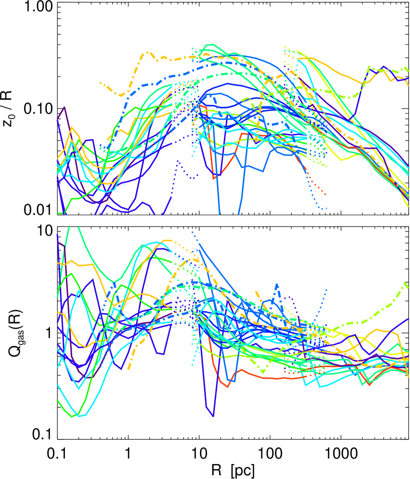
Our interpretation and analysis of the inflow rates assumes that the gas resides in a self-gravitating, at least modestly thin, disk. To demonstrate this explicitly, Figure 10 shows the vertical scale height and Toomre Q parameter of the gas as a function of radius. For each simulation, at a given radius $R$ we determine the scale height $z_{0}$ of the gas by fitting the gas density distribution to a Gaussian with dispersion $z_{0}$ (after projecting to the plane perpendicular to the net angular momentum vector). At large radii, there is scatter owing to the difference between mergers (with sizeable $z_{0}/R$) and unstable disks. From $\sim 1-100\,$pc, $z_{0}/R$ ranges from $\sim 0.05-0.25$; this is determined by our assumed ISM equation of state, as well as kinematic features such as twists and misalignments. At the smallest radii $z_{0}/R$ begins to decrease rapidly because the potential is increasingly dominated by the BH (the circular velocity increases but the maximum sound speeds are finite). Note that, at all radii, the minimum SPH smoothing length $h_{\rm sml}\lesssim z_{0}$, so that the disk thickness is at least modestly resolved. Our simulated disks are always reasonably thin because the cooling time is always short compared to the dynamical time, so that the sound speed in the simulation reliably tracks that of our subgrid model.

Figure 10 also shows the Toomre $Q$ parameter of the gas, defined as $Q\equiv c_{s}\,\kappa/\pi\,G\,\Sigma_{d}$, where $\kappa$ is the local epicyclic frequency and $\Sigma_{d}$ is the total surface density of the disk (gas plus stars). With some scatter, systems largely lie near $Q\sim 1$. This is broadly expected for self-regulating disks; in the simulations, $Q\sim 1$ is a consequence of star formation, the assumed stellar feedback, and gravitational dynamics.

4.1 Gas Density Profiles

Figure 11: Gas surface density $\Sigma_{\rm gas}$ at different radii as a function of time, for the simulations shown in Figure 5. Top: Large scale galaxy merger simulation. The box shows the time interval re-simulated in the panel below. Middle: Intermediate-scale re-simulation. The box again shows the time interval for the smaller scale re-simulation. Bottom: Nuclear-scale re-simulation. Comparing with Figure 5, high inflow rates are generally correlated with higher local surface densities, but the relation is not one-to-one.

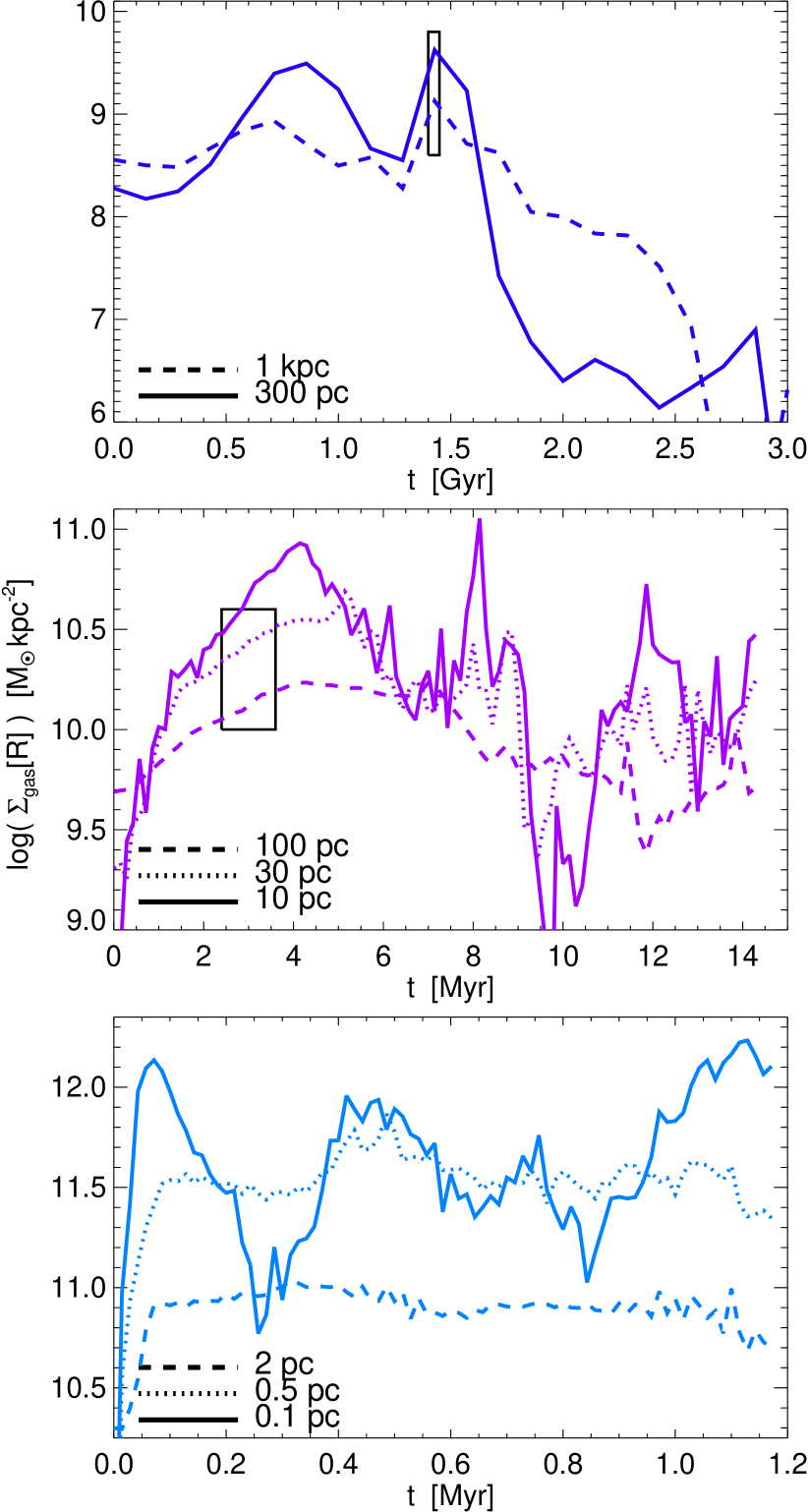
Figure 11 shows the gas surface density as a function of time, at different radii, in the high-inflow simulation from Figures 2 & 5. Comparison of Figures 5 & 11 clearly indicates that there is a reasonable correlation between high inflow rates and high gas surface densities at the same radii. However, the correlation is not necessarily one-to-one because of the complex time-dependent dynamics on small scales. In some cases, the inflow leads the high surface density (e.g., $0.4\,$Myr at $0.1\,$pc or $\sim 2-4\,$Myr at $10\,$pc), in which case the large $\dot{M}$ causes the high $\Sigma$, rather than the other way around. Occasionally, $\dot{M}$ and $\Sigma$ can even be anti-correlated (e.g., at $10\,$Myr on $10\,$pc scales).

Figure 12: Left: Gas surface density profiles during the strong inflow phases, i.e., when the accretion rate at small radii peaks. Each solid line denotes a different simulation, with dotted lines showing the radii near the boundaries of our re-simulations, where the exact profile shape is suspect; colors correspond to initial gas fractions as in Figure 13. Thick lines are the ultra-high resolution simulations. Each simulation consists of re-simulations of the nuclear dynamics during gas-rich galaxy-galaxy mergers, as in Figures 5 & 11. Dashed red line shows the initial gas density profile of the large-scale simulations (run b3ex(ic) in Table 1). The gas density profile is quasi-steady over the entire active phase, with star formation offsetting inflow; the time variation in $\Sigma_{\rm gas}$ for one example is shown in Figure 11. Right: Gas surface density profiles for simulations of isolated barred-disk galaxies and the corresponding re-simulations. In cases with a very small pre-existing bulge, the central gas density can increase by an order of magnitude, but not the $2-4$ orders of magnitude seen in the left panel.

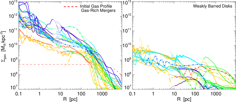
Figure 12 shows the gas density profiles as a function of radius for our ensemble of simulations (including the individual simulations shown in Figures 5 & 6); for the gas-rich systems in the left panel, these surface density profiles are at the peak of activity, i.e., when $\dot{M}$ is relatively high. During these active phases, the gas reaches a quasi-equilibrium density distribution. For a given annulus, the net accretion rate to smaller radii is typically a small fraction of the total rate at which gas is supplied to that annulus. Thus to first approximation, the surface density can be estimated by considering the competition between star formation and inflow in a given annulus. If the star formation rate surface density scales $\propto\Sigma_{\rm gas}^{3/2}$, as in Kennicutt (1998), then setting the star formation rate inside some radius equal to the time-averaged inflow rate $\dot{M}_{\rm in}$ gives an expected $\langle\Sigma_{\rm gas}\rangle\propto\dot{M}_{\rm in}^{2/3}\,R^{-4/3}$. Given $\dot{M}_{in}\propto R^{1/2}$, which is reasonably consistent with Figure 5, this implies $\Sigma_{\rm gas}\propto R^{-1}$, similar to the results for the gas rich systems in Figures 11-12 (although slightly steeper than the numerical results). There is of course significant variation: we show the results from our large suite of simulations to emphasize the variation introduced by initial and boundary conditions, treatment of star formation and gas physics, etc., but also to highlight the robust average behavior and the dependence on global quantities such as gas fraction and inflow rate at larger radii (see Fig. 13 for the color scheme).

Note that the gas surface densities achieved on small scales can be extremely large, $\sim 10^{11}-10^{12}\,M_{\sun}\,{\rm kpc^{-2}}$ in the central $\sim 0.1-10\,$pc; this is comparable to, or even somewhat larger than, the highest-surface density stellar systems known (Hopkins et al., 2009e; Hopkins & Hernquist, 2009). And it is a factor of $\sim 10^{4}$ larger than the initial gas surface density at small radii (shown in Fig. 12 for comparison)! Assuming that a significant fraction of the gas eventually turns into stars, the relic stellar density profiles expected from these gas-rich simulations are similar to the observed profiles of nearby “cusp” ellipticals (e.g., Kormendy et al., 2009), which are indeed believed to be direct descendants of gas-rich mergers. However, estimating the “final” stellar profile at small radii, where our simulations are run for only a modest number of local dynamical times, requires a careful correction for the effects of duty cycle, so we defer a more detailed comparison to future work.

Figure 12 (right panel) also shows the gas surface density profiles for cases in which the initial large-scale gas inflows are not strong (e.g., Fig. 6). Most of these simulations represent either extremely gas-poor mergers or (more commonly) systems that are weakly bar unstable or bar unstable but with significant bulge components (such that bars form efficiently, but inflow stalls at a large inner Linblad resonance). In such cases, the large-scale dynamics cannot increase the gas density at sub-kpc scales very far above the initial value of $\sim 10^{8}-10^{9}\,M_{\sun}\,{\rm kpc^{-2}}$. Without this enhancement, the system is stable against secondary instabilities, and so there is little gas inflow at small radii (e.g., Fig. 6).

In both the strong and weak inflow cases in Figure 12, our small subset of ultra-high resolution simulations (dot-dashed thick lines; 6 galaxy-scale runs that resolve down to $\sim 10\,$pc, and 5 intermediate-scale runs that extend to $<1$ pc) are fully consistent with the larger suite of lower resolution re-simulation runs. These high resolution simulations have continuous inflow from large to small radii, and can therefore be run self-consistently for a much larger number of dynamical times than our typical resimulation. In spite of this advantage, we find that our resimulation technique yields very similar results.

5 Conditions for (In)Stability

In the preceding sections, we have presented results for cases in which gas inflow from large scales both is, and is not, sufficient to trigger secondary instabilities at small radii, leading to efficient gas inflow down to $\sim 0.1\,$pc. Here we provide a more quantitative assessment of the conditions under which there is significant inflow of gas to sub-pc scales.

Figure 13: Inflow strengths as a function of bulge to total ratio (B/T) for several initial gas fractions (colors) and ISM equations of state $q_{\rm eos}$ (symbol type), for a subset of our simulations. Large symbols in each refer to the subset of ultra-high resolution simulations. Top: Total gas mass inside an inner radius of $10\,$pc (left; from our intermediate-scale re-simulations) or $0.1\,$pc (right; from our nuclear-scale re-simulations), near the peak of accretion in each simulation. “Bulge” (B) refers to any spherical term in the potential (bulge+halo+black hole). Middle: Gas inflow rate through the relevant inner radius. Solid points denote the time-averaged inflow rate over the full re-simulation while open points are the maximum seen in any individual snapshot (to give some sense of the duty cycle). Bottom: Amplitude of the dominant non-axisymmetric mode in the stars (generally $m=2$ at intermediate scales, $m=1$ at nuclear scales), averaged over the peak/strong inflow phase. Inflow properties scale broadly with $B/T$ as expected, but the large scatter and sensitivity to other parameters makes a large parameter survey critical.

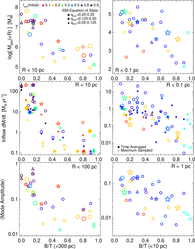
Figure 13 shows how several different measures of the efficiency of angular momentum transport and gas inflow depend on the initial gas fraction $f_{\rm gas}$ and the “bulge” to total ratio $B/T$ – the same parameters that strongly influence the morphology of the gas (Fig. 3 & 4). We show results for a few different equations of state $q_{\rm eos}$ (see Fig.1). The quantities we use to define the efficiency of gas inflow are the gas mass within $10$ and $0.1\,$pc $M_{\rm gas}(<R)$ (top panel), the inflow rates within the same radii (middle panel) and the formal amplitude of the non-axisymmetric gravitational perturbations at $\sim 1$ and $\sim 100$ pc (bottom panel). For the inflow rate (middle panel), we show both the time average and “peak” values to convey the variability as a function of time in the simulation.

The mode amplitude is measured in the standard fashion from the surface density distribution at a given radius, using

$$|a_{m}(R,t)|=\frac{||\int_{0}^{2\pi}\Sigma(R,\phi)\,\exp{(i\,m\,\phi)\,{\rm d}\phi}||}{\int_{0}^{2\pi}\Sigma(R,\phi)\,{\rm d}\phi}\ .$$ (5)

We measure the amplitude from the stellar disk since it is slightly more robust to local clumping, but using the gas surface density gives similar results. For simplicity, we show the results for the largest-amplitude mode in each case, but this is almost always $m=1$ in the nuclear-scale simulations (right panels) and an $m=2$ bar or $m=1$ spiral in the intermediate-scale simulations (left panels). We measure the relevant amplitude at radii slightly larger than the radii where the inflow is measured, since it is this non-axisymmetry that drives the inflow (it is also somewhat less noisy at larger radii).

The “bulge-to-total” ratio in Figure 13 is defined as the mass fraction in all spherical components within the specified radius, since these all serve to suppress instability in the same manner (e.g. any black hole, bulge, halo, and/or nuclear star cluster would qualify). Gas fraction is defined as the gas fraction of the disky component within the same radius.

Figure 13 shows clearly that there is a very strong trend of inflow strength with $B/T$, in the expected sense. Strongly disk-dominated systems have characteristic inflow rates 3 orders of magnitude higher than strongly “bulge-dominated” systems; likewise mode amplitudes and gas masses inside small radii are higher by $1-2$ orders of magnitude.

There are several interesting additional results in Figure 13. First, within the range of $q_{\rm eos}$ that we consider (motivated by the observations in Figure 1), the inflow properties do not depend significantly on the ISM physics. This is consistent with our previous arguments; so long as the sub-resolution model is sufficient to prevent catastrophic fragmentation and runaway star formation, gravitational torques that are reasonably independent of the ISM microphysics dominate the angular momentum redistribution. Note that there is also no distinguishable difference between the results of our ultra-high resolution runs (shown with large symbols) and our standard resimulations. Second, the inflow properties depend much more strongly on B/T than on the initial gas fraction; this is because the stellar disk generates the same instabilities as the gas disk. In fact, the collisional nature of gas means it cannot support certain strong modes (Toomre, 1977), so the transport can be less efficient in the fully gas-dominated limit (the gas-rich systems modeled here often do not develop strong modes until a non-trivial fraction of the gas has turned into stars).

Third, there is considerable scatter at all $B/T$. This is in no small part due to the time-variable nature of the small scale dynamics (§3). In addition, however, a quantity such as $B/T$ is not a global invariant; it depends on both position and time in these simulations. As such, some simulations with a given $B/T$ at the specified radius can have a larger or smaller $B/T$ at some larger radius, leading to more or less efficient inflow from those scales that in turn leads to more or less efficient inflow to smaller scales. Identifying $B/T$ at a given radius and time is thus a crude measure of stability. Moreover, the torques and inflow rates depend on the precise structure of the modes involved; a significant portion of the scatter in Figure 13 reflects the difference between e.g. bars, spiral arms, and loosely or tightly-wrapped waves. This large scatter highlights the importance of using a large suite of simulations to conduct parameter surveys and build statistical samples – any individual system, studied for a small amount of time, can be highly non-representative.

5.1 Intermediate (sub-kpc) Scales

For the intermediate scale results shown in the left panel of Figure 13, we can gain some analytic understanding of the behavior by following Shlosman et al. (1989), who discuss the criteria for secondary instabilities (“bars within bars”). It is well established that a self-gravitating disk becomes unstable to large-scale gravitational modes roughly when the Ostriker-Peebles criterion is met, i.e., when $T_{\rm rot}/|W|>t_{\rm crit}$, where $T_{\rm rot}\sim M_{d}\,V_{c}^{2}$ is the kinetic energy of rotation (in the rotationally supported – i.e. kinematically cold – component), $|W|\sim G\,M^{2}/R$ is the potential energy, and $t_{\rm crit}$ is a threshold value $\simeq 0.15-0.26$, depending on the nature of the instability (e.g., Bardeen 1975; Aoki et al. 1979). If a mass fraction $f_{d}=1-B/T$ is in the disk, the condition for instability generically becomes

$$f_{d}>f_{\rm crit}(t_{\rm crit},\,a/R)$$ (6)

where $a$ is the bulge scale length, $R$ is the disk scale length, and the exact functional form of $f_{\rm crit}$ depends on the profiles of the disk and bulge. For Kuzmin and Plummer profiles for the disk and bulge, respectively, we find that this instability criterion becomes

$$\frac{M_{d}[<R]}{M_{b}+M_{d}[<R]}> \left(\frac{3\pi\,t_{\rm crit}}{4[1-2\,t_{\rm crit}]}\,\frac{R}{a}\right)^{1/2} (R\ll a)$$ (7)

$$\left(\frac{3\pi\,t_{\rm crit}}{16}\,[1+(a/R)^{2}]\,\frac{R}{a}\right) (R\sim a)$$ (8)

where $M_{d}[<R]$ is the total (stars + gas) disk mass within $R$ and $M_{b}$ is the total bulge mass.

If the disky material of interest has a scale-length comparable to that of the bulge (generally true for the intermediate-scale simulations here), equation (6) simply becomes $B/T\lesssim 1-t_{\rm crit}\simeq 0.7-0.8$. This is reasonably consistent with the fact that the inflow rate and interior gas mass in the intermediate scale simulations in Figure 13 (left column) asymptote for $B/T\gtrsim 0.6-0.7$.

Shlosman et al. (1989) show that an initial gas disk must be compressed to at least $R_{\rm new}/R_{i}\sim(1.0-2.5)\,f_{\rm gas}^{2}/[1+0.2\,(B/T)^{2}]$ to satisfy equation (6), again for systems in which the disk and bulge initially have similar scale-lengths. For the case of major mergers, we can compare this to Covington et al. (2008) and Hopkins et al. (2009a, c)’s estimates of how much angular momentum the gas loses during the merger. These authors find that the gas often inflows until it becomes self-gravitating – as a result, secondary bar instabilities should be ubiquitous. More quantitatively, they find $R_{\rm new}/R_{i}\approx f_{\rm gas}/(1+f_{\rm gas}/f_{0})$ with $f_{0}\approx 0.2-0.3$. Using this, we estimate that mergers with reasonable gas fractions $\gtrsim 0.3-0.5$ will lead to secondary instabilities and rapid inflow. For isolated disk galaxies with bars, the critical criterion is whether the inner Linblad resonance lies inside or outside of $R_{\rm new}$; this will generally not be true in low-$f_{\rm gas}$ or high-$B/T$ systems.

5.2 Nuclear (pc) Scales

Inside the radius where the BH begins to dominate the gravitational potential, it becomes increasingly difficult for system to be globally gravitationally unstable in the sense of $T_{\rm rot}/|W|>t_{\rm crit}$. Specifically, in the potential of the BH this criterion implies that the disk would no longer be unstable inside a radius $R_{\rm min}\sim 10\,{\rm pc}\,(M_{\rm BH}/10^{8}\,M_{\sun})^{1/2}\,(\Sigma_{d}/10^{11}\,M_{\sun}\,{\rm kpc^{-2}})^{-1/2}$. This confirms our earlier claims (e.g., §3.3) that the character of the instabilities responsible for angular momentum transport must change near the BHs radius of influence. Indeed, we see numerically that the transport on small scales is dominated by $m=1$ modes (e.g., Fig. 4).

A full discussion of the origin of the $m=1$ modes is beyond the scope of this paper; we will present a detailed analytic analysis (in simplified BH+disk models) of their structure, growth rates, and pattern speeds in future work (in preparation). We can, however, present a simple analysis indicating how we believe the modes arise. For $m=1$ modes, $\Omega-\kappa/m\rightarrow 0$ in a Keplerian potential. It is well-known that this allows very low frequency (low pattern speed $\Omega_{p}$) modes to be present in a Keplerian potential (e.g., Tremaine 2001). Moreover, Tremaine (2001) showed that the only modes that can be global and exert coherent strong torques over a large dynamic range in a quasi-Keplerian potential are these $m=1$ modes. We find that the modes in the simulations indeed have small $\Omega_{p}$, i.e., $\Omega_{p}\ll\Omega$ and $m=1$, deep in the potential well of the BH. Note that for a collisionless particle, rather than the stellar+fluid disks of interest here, this simply corresponds to a standing elliptical Keplerian orbit. Small $\Omega_{p}/\Omega$ (and wavenumber $m=1$) is important because it implies near-resonance conditions at small radii; this allows the stars to produce strong torques on the gas, which drives orbit crossings, shocks, and angular momentum loss, even when the mass of the disk at small radii is much less than the BH mass (see e.g. Chang et al., 2007). Following Tremaine (2001) and expanding the equations of motion for a linear mode in a nearly-Keplerian potential (in the WKB limit) it is straightforward to show that the magnitude of the induced velocities ($\delta v/V_{c}$) from a given mode scale as $\delta v/V_{c}\sim(\delta\Sigma/\Sigma)\,M_{d}(<R)/M_{\rm BH}=|a|\,M_{d}(<R)/M_{\rm BH}$ for all $m\neq 1$; for $m=1$, however, $\delta v/V_{c}\sim|a|$. In other words, the conventional wisdom that torques from global modes are strongly suppressed in the spherical potential of a BH is generally true, but the resonance condition that $\kappa\simeq\Omega$ in Keplerian potentials allows for large coherent eccentricities, self-gravitating collective effects, and torques from $m=1$ modes at arbitrarily small disk-to-BH masses. As a result, although we certainly see higher-$m$ modes in our small-scale simulations, the global structure is almost always dominated by a coherent global $m=1$ eccentric disk.

However, Tremaine (2001) also showed that slow modes with pattern speeds $\Omega_{p}\ll\Omega$, are linearly stable in quasi-Keplerian potentials. How, then, do these modes arise in the simulations? To start, we consider the dispersion relation for linear waves in the WKB limit (see e.g. Lau & Bertin, 1978), which is given by

$${\Bigl{(}}\frac{\omega-m\Omega}{\Omega}{\Bigr{)}}^{2}=1+\nu-2\tilde{f}_{d}A\left(|kr|^{2}+m^{2}\right)^{1/2}+A\left(|kh|^{2}+{\frac{m^{2}h^{2}}{r^{2}}}\right)$$ (9)

where

$$\tilde{f}_{d}\equiv\frac{\pi\,\Sigma_{d}\,R^{2}}{M_{\rm enc}(<R)}\approx\frac{M_{d}(<R)}{M_{\rm tot}(<R)},$$ (10)

$$A=1+{\frac{2m^{2}(3-\nu)}{(\nu+1)(|kr|^{2}+m^{2})}},$$ (11)

$$\nu\equiv 1+2\,\frac{\partial\ln V_{c}}{\partial\ln R}\approx\frac{{\rm d}\ln M_{\rm enc}(<R)}{{\rm d}\ln R}\ ,$$ (12)

and $h=c_{s}/\Omega$ is the disk thickness. We now consider the limit of equation (9) such that $kr$ is modest. Of course, our analytic treatment of such quasi-global gravitational modes should be considered with due caution, as the WKB approximation necessary to derive the dispersion relation is not justified. But this nevertheless points towards the conditions under which global gravitational instability may be present. In this limit, equation (9) will have growing modes if the right-hand side is negative, which for a cold disk ($h\ll r$) requires

$$\tilde{f}_{d}>\frac{1}{2\,m}\,\frac{(1+\nu)^{2}}{7-\nu}\ .$$ (13)

As $\nu\rightarrow 0$, i.e., as the potential becomes Keplerian, equation 13 suggests that $m=1$ modes can become unstable when $\tilde{f}_{d}\gtrsim 0.1$. This is consistent with the fact that we find the $m=1$ modes at nearly all $B/T$ (Fig. 13). Equation 13 also allows for the instability of higher-$m$ modes, but these cannot exert coherent strong torques on the gas, nor can they propagate efficiently to small radii, so they do not dominate the structure or inflows we see in our simulations.

Because the disk in general will have more mass at large radii, any instability will grow outside-in; for massive disks, the most-unstable point is where $M_{d}(<R)\sim 0.5-1\,M_{\rm BH}$ ($\tilde{f}_{d}\sim 1/3-1/2$). Here modes can grow on a dynamical time. Equation 9 shows that this growth is for fast modes: overstabilities with Re($\omega$) $\sim m\,\Omega$. In the simulations, the slow modes typically dominate the torques at sub-pc scales. However, we find that the fast mode itself drives the slow modes. Specifically, the $m=1$ mode first appears around the most unstable point $R_{\rm crit}$ predicted above, where $M_{d}(<R_{\rm crit})\sim 0.5-1\,M_{\rm BH}$. This rapidly leads to an eccentric disk at these radii. As the instability causes gas to lose angular momentum, the gas falls inwards, and begins turning into stars. The eccentric mass distribution at $R_{\rm crit}$ then in turn efficiently induces a similar eccentricity at smaller radii. As noted in Tremaine (2001), the $m=1$ slow mode may be linearly stable, but it can be excited in the first place – and will be long-lived – in response to an external asymmetry in the potential. Our interpretation of the simulations is that the unstable self-gravitating disk near $\sim R_{\rm crit}$ provides the asymmetry that generates the slow, low pattern speed, $m=1$ mode at smaller radii. The pattern speed $\Omega_{p}=\Omega(R_{\rm crit})$ is conserved as the mode moves in, but the circular speed $\Omega(R)$ is rapidly increasing at smaller radii near the BH, so the mode at small radii is indeed a slow mode – for the typical parameters here, the pattern speed is $\Omega_{p}\sim 1-5\,{\rm km\,s^{-1}\,pc^{-1}}$, set by the circular speeds at $\sim 10-100\,$pc, where $M_{d}(<R)\sim M_{\rm BH}$ (for comparison, $\Omega\gtrsim 1000\,{\rm km\,s^{-1}\,pc^{-1}}$ at $R<1\,$pc). The slow mode at small radii responsible for the angular momentum transport is therefore not a local small-scale instability, but part of a global instability beginning at larger radii. In the future, we plan to explore the origin of this global $m=1$ mode in more detail. Calculating the dynamics of the gas and stars, and including self-gravity and star formation, are all important for capturing the inward propagation of these modes.

Similar $m=1$ modes have been studied previously as a mechanism for accretion in fluid disks (Adams et al., 1989; Shu et al., 1990; Ostriker et al., 1992; Bournaud et al., 2005), both in the galactic context and in proto-planetary or proto-stellar disks (e.g., Banerjee et al., 2004; Boley et al., 2006; Vorobyov & Basu, 2006; Vorobyov & Basu, 2009; Krumholz et al., 2007; Cai et al., 2008). In a purely gaseous disk, wave packets can propagate through the OLR to $r\rightarrow\infty$, eventually becoming simple sound waves (Adams et al., 1989). Because the waves can freely escape to the outer boundary, infinite pure gaseous disks in nearly-Keplerian potentials do not support strong growing $m=1$ modes, and the mode growth is quite sensitive to the description of the disk boundary. However, for a stellar disk, the mode cannot propagate beyond the OLR where $\Delta\equiv\kappa^{2}-m\,(\Omega-\Omega_{p})^{2}=0$. Refraction of the stellar waves at this boundary is important, and implies that global $m=1$ modes can grow even when the disk extends to $R\gg R_{\rm OLR}$. As a result, we shall show in subsequent work that the $m=1$ modes in quasi-Keplerian stellar disks are relatively insensitive to the outer boundary conditions. This is also implicit in Tremaine (2001), where for many of the modes the outer radius of the disk could be arbitrarily large. The ability of stellar $m=1$ modes to grow more readily again highlights the importance of considering the two component stellar + gas system when considering gas inflow in galactic nuclei.

6 Accretion versus Star Formation

Figure 14: The predicted relationship between the BH accretion rate (BHAR) and the star formation rate (SFR) inside a given radius. For each simulation, we plot the SFR integrated within the indicated projected radius, at different times during the simulation, compared with the $<0.1\,$pc BH accretion rate from appropriate re-simulation. The characteristic timescale for variability at small radii – which sets the variability in the BHAR – is much shorter than the corresponding timescale at large radii; at fixed SFR, each system can thus have a variety of BHARs. Nevertheless, the BHAR correlates with SFR, with the least scatter for the nuclear star formation (upper left). The correlations seen here are a natural consequence of the fact that high gas densities, and thus high star formation rates, are necessary to trigger secondary instabilities and drive accretion on small scales.

Given the gas inflows modeled here, our results imply a correlation between the accretion rate onto the central BH – and hence the AGN luminosity – and the star formation rates on larger scales. Figure 14 shows this correlation for a number of our simulations. We take the inflow rate at $0.1$ pc as the AGN accretion rate, which corresponds to a bolometric luminosity of

$$L_{\rm bol,\,AGN}=\epsilon_{r}\,\dot{M}_{\rm BH}\,c^{2}\approx 5.7\times 10^{45}\,{\Bigl{(}}\frac{\epsilon_{r}}{0.1}{\Bigr{)}}\,{\Bigl{(}}\frac{\dot{M}_{\rm BH}}{M_{\sun}\,{\rm yr^{-1}}}{\Bigr{)}}\,{\rm erg\,s^{-1}}\$$ (14)

where the radiative efficiency is $\epsilon_{r}=0.1$. Figure 14 compares the BH accretion rate to the total star formation rate inside a (projected) radius $R$, at a few representative radii: true nuclear scales ($R<10\,$pc), more readily observable nuclear scales ($R<100\,$pc), the smallest scales observable in most moderate to high-redshift systems ($R<1\,$kpc), and the total star formation rate, integrated over all radii ($R\rightarrow\infty$). For each point, in Figure 14, the projected SFR$(<R)$ is technically the median over $\sim 100$ sightlines, but projection effects are negligible. For the larger radii, we measure the SFR in an appropriate intermediate or galaxy-scale simulation. The BH accretion rate is then determined from that in the appropriate re-simulation or set of re-simulations matched to the galaxy scale simulation central properties at the given time. Because a given dynamical time in a galaxy-scale simulation corresponds to many dynamical times (and simulation outputs) on very small scales, the number of points is larger in the plots going out to larger scale.

Not surprisingly, Figure 14 shows that there is a correlation between accretion rate and star formation rate, on all scales. There is significant scatter in this correlation, although the scatter is less when the SFR is evaluated inside a small nuclear annulus. If we assume a linear proportionality between BH accretion rate and star formation rate in some annulus, we find

$$\dot{M}_{\rm BH} \sim\dot{M}_{\ast}(R<10\,{\rm pc})$$ (15)

$$\sim 0.1\,\dot{M}_{\ast}(R<100\,{\rm pc})$$ (16)

$$\sim 0.03\,\dot{M}_{\ast}(R<1\,{\rm kpc})$$ (17)

$$\sim 0.003\,\dot{M}_{\ast}({\rm total})$$ (18)

for the median relation in the simulations, which corresponds to a bolometric luminosity ratio of $L_{\rm bol,\,SF}/L_{\rm bol,\,AGN}\sim(0.01,\,0.1,\,0.3,\,2.5)$ at $(R<10\,{\rm pc},\,R<100\,{\rm pc},\,R<1\,{\rm kpc},\,R<\infty)$, respectively, or a ratio of the star formation-powered infrared luminosity to the hard X-ray luminosity from the AGN of $L_{\rm IR,\,SF}/L_{\rm HX,\,AGN}\sim(0.2,\,2,\,6,\,60)$ in the same annuli.

In greater detail, the correlations are not precisely linear. Parameterizing the correlation between star formation and BH accretion as a power-law, $\dot{M}_{\rm BH}\propto\dot{M}_{\ast}^{\alpha}$, we find that the correlations above are approximately valid for $\dot{M}_{\rm BH}\sim 0.1-10\,M_{\sun}\,{\rm yr^{-1}}$, but $\alpha$ changes from near-linear at small scales ($R<10\,$pc) to somewhat super-linear ($\alpha\sim 1.5$) on large scales. For the total star formation rate, we find

$$\dot{M}_{\rm BH}\sim 0.5\,{M_{\sun}\,{\rm yr^{-1}}}\,{\Bigl{(}}\frac{\dot{M}_{\ast}}{50\,{M_{\sun}\,{\rm yr^{-1}}}}{\Bigr{)}}^{1.5}\ .$$ (19)

However, we caution that our simulations do not include the appropriate physics to resolve the variety of processes that can produce low accretion rates $\ll 0.1\,M_{\sun}\,{\rm yr^{-1}}$, nor do they sample a large regime of galaxies with total star formation rates $\lesssim 1\,M_{\sun}\,{\rm yr^{-1}}$, so the fits above should not be used in the limits of weak accretion and star formation. The qualitative point is nonetheless important: non-axisymmetric instabilities due to self-gravity become inefficient at low gas densities (low star formation rates), and so other mechanisms must be important for fueling at least some of the low-luminosity AGN population.

It is notable that even during the active phases modeled here, the average relation between accretion rate and total SFR is such that the systems are most often not AGN dominated in a bolometric sense (although the two are certainly comparable, in these phases). In other words, even the most active systems will be consistent with SFR-dominated properties except for a small fraction of the time; this is consistent with observations such as the FIR-radio correlation (Walter et al., 2009; Riechers et al., 2009; Wang et al., 2008). However, the scatter in accretion rates at fixed SFR is large, and most of the growth in BH mass comes from the rare, short-lived times when the systems scatter to higher $L_{\rm AGN}/L_{\rm SF}$. Roughly, we can estimate these duty cycles with the scatter in Figure 14 – about $\sim 30\%$ of the systems in “peak” AGN phases have sufficient accretion rates ($\dot{M}_{\rm BH}\gtrsim 0.01\,\dot{M}_{\ast}$) so as to be AGN-dominated.

The predictions in Figure 14 can be compared to a number of observations. Wu & Cao (2006) compile total star formation rate estimators in $\sim 100$ nearby AGN ranging in luminosity from LINERS ($\dot{M}_{\rm BH}<0.01\,M_{\sun}\,{\rm yr^{-1}}$) to PG quasars ($\dot{M}_{\rm BH}\sim 1-5\,M_{\sun}\,{\rm yr^{-1}}$). The sample details are discussed in Satyapal et al. (2005), but the authors find they are reasonably robust to the choice of SFR or BH accretion rate indicator. Silverman et al. (2008) consider a similar compilation in more luminous systems in the COSMOS survey, spanning a redshift range $z\sim 0.3-1.1$. At total SFR values $>10\,M_{\sun}\,{\rm yr^{-1}}$, these samples agree fairly well. Specifically, for $\dot{M}_{\ast}\sim 10-1000\,M_{\sun}\,{\rm yr^{-1}}$, these different compilations are consistent with a median $\dot{M}_{\rm BH}\sim 0.001-0.01\,\dot{M}_{\ast}$, with factor of $\sim 3$ dispersion; this is quite similar to our results shown in Figure 14. On the other hand, Ho (2005) used OII line emission to argue that the star formation rate associated with luminous type 1 AGN is at best comparable to the BH accretion rate, inconsistent with the median integrated galaxy predictions in Figure 14. This may be because obscuration makes OII an imperfect proxy for star formation in dense, obscured, starbursts. In addition, luminous Type 1 AGN are probably, by selection, on the tail end of the BHAR/SFR distribution (and could in principle be in an AGN feedback-dominated stage of evolution not modeled here). Indeed, Kim et al. (2006) followed up Ho’s work and found enhanced star formation in type 2 quasars, similar to our predictions here.

Wang et al. (2007) consider spatially resolved estimates of nuclear luminosity and emission-line (SFR) profiles in a range of Seyferts and quasars (mostly at low redshift) at spatial scales from $\sim 0.05-3\,$kpc (see Imanishi, 2002, 2003; Imanishi & Wada, 2004). Their results are similar to those in a variety of other studies (see e.g. Kauffmann et al., 2003; Kewley et al., 2006; Evans et al., 2006; Schawinski et al., 2009). At both $R<100\,$pc (where the observations span a dynamic range in SFR$(<100\,{\rm pc})\sim 0.1-10\,M_{\sun}\,{\rm yr^{-1}}$) and $R<1\,$kpc (SFR$(<1\,{\rm kpc})\sim 1-100\,M_{\sun}\,{\rm yr^{-1}}$), our results are reasonably consistent with these observations, in both normalization and scatter. A small sample is studied at extremely high resolution in Davies et al. (2007), where star formation and AGN luminosity are resolved at $\sim 10-30\,$pc scales. They find that, within these radii, the luminosity from star formation is $\sim 1-5\%$ of that from the BH, again consistent with our prediction here.

7 Discussion

We have presented high resolution smoothed particle hydrodynamic simulations of the dynamics of gas in the central regions of galaxies, in order to study gas inflow from galactic scales $\sim 10\,$kpc down to the scales of a canonical AGN accretion disk ($\sim 0.1\,$pc). We use the properties of galactic-scale simulations – both mergers and isolated galaxy disks – to initialize new higher resolution “re-simulations” that focus on the $\lesssim 100$ pc dynamics. This technique is then applied a second time to follow the gas to $\sim 0.1$ pc. By intention, our calculations do not employ particle splitting and are not all exact realizations of the small-scale dynamics associated with a single, specific larger-scale simulation. Our “re-simulations” should not be taken as such an exact realization. Instead, since it is not practical to directly solve the “full” problem (from $\sim 10\,$kpc to $10^{-5}\,$pc), we have focused on understanding and isolating the key physics involved. To provide a more physical model, however, we use initial conditions drawn from a variety of larger galaxy-scale simulations, rather than an ad hoc set-up. This approach allows us to systematically survey, for the first time, how a large variety of initial conditions and galaxy properties affect gas dynamics in galactic nuclei.

It is still not feasible, with any numerical scheme, to simultaneously model the small scales of an AGN accretion disk and those of a galaxy for cosmological timescales. For this reason, direct “zoom-in” approaches have thus far been fairly limited, usually evolving each region for just a few local dynamical times. Our numerical approach attempts to overcome this severe limitation. First, the smallest regions of each simulation are simulated for many local dynamical times. Even more importantly, we quantity the dynamics on small scales using $\sim 100$ simulations of a large range of initial conditions and galaxy properties This approach does not require an exact mapping between one large-scale simulation and another on smaller scales (although we often interpret our results in this manner). For example, even if our nuclear-scale simulations of the central $\sim 100\,$pc of a galaxy are not self-consistently matched to those of a specific larger-scale simulation, they still represent valid simulations of a given set of initial conditions of a bulge+stellar disk+gas disk+BH system, evolved for many dynamical times. As such, we can still use them to understand the physics of angular momentum transport and BH fueling at these radii (given these initial conditions). This methodology allows us to survey a wide range of initial conditions and galaxy properties and isolate the physical parameters that are most important for the physics of gas inflows on small scales in galactic nuclei. We have also checked our ”re-simulation” approach by carrying out a small number of ultra-high resolution simulations that bridge the gap between different resimulated regions; we find in all cases that these ultra-high resolution simulations validate our resimulation methodology.

Our calculations demonstrate that for sufficiently gas-rich, disk-dominated systems, which have a large inflow of gas into $\sim$kpc scales, there is a cascade of non-axisymmetric gravitational instabilities that ultimately produces BH accretion rates as high as $\sim 10\,M_{\sun}\,{\rm yr^{-1}}$ at $\lesssim 0.1$ pc (Fig. 13). Moreover, we have explicitly shown that these conditions are satisfied during major mergers of gas-rich galaxies, thus providing theoretical support for the connection between mergers and BH growth. It is, however, also important to stress that our work only implies that galaxy mergers are a sufficient condition for fueling a central quasar, not that they are necessary: similar inflows can be obtained in isolated gas-rich, bar or spiral wave-unstable galactic disks.

In broad terms, our results support the “bars within bars” scenario proposed in Shlosman et al. (1989). However, we show that the secondary instabilities on intermediate scales ($\sim 10-100$ pc) exhibit a diverse range of morphologies, including standard nuclear spirals, bars, rings, barred rings, one or three-armed spirals, and irregular/clumpy disks and streams (Fig. 2 & 3). This is very important for comparing to real galaxies: observations have generally found that nuclear bars are not ubiquitous in AGN (perhaps not substantially more common than in non-active systems). However, these same observations have found that some form of asymmetric nuclear structure is ubiquitous, with the most common features being nuclear spirals and rings very similar to those seen in Figure 3 (see Martini & Pogge, 1999; Martini et al., 2003; Peletier et al., 1999; Knapen et al., 2000; Laine et al., 2002; Knapen et al., 2002; Greene et al., 2009, and references therein). Our work shows that these observations are not necessarily in conflict with the hypothesis that gravitational torques dominate inflow on sub-kpc scales in AGN. Rather there is a large diversity in the observational manifestation of these gravitational torques. “Bars within bars” should not be taken too literally. Instead a more accurate characterization would be: “it’s non-axisymmetric features all the way down” (or “stuff within stuff”).

This diversity in observational appearance owes both to the effects of global parameters such as gas fraction and bulge-to-total ratio, and more subtle variations induced by the relative scale lengths of disks and bulges, the precise profile shapes, and the thickness/dispersion in the sub-kpc bulge, stellar disk, and gaseous disk components. Observationally, these parameters are all seen to vary considerably even in isolated galaxies, let alone in chaotic merging systems; as a result, we expect the morphological diversity exhibited in Figures 2 & 3 to be the norm.

Once the gas reaches the BH radius of influence ($\sim 10\,$pc for a typical $\sim L_{\ast}$ system), the potential becomes quasi-Keplerian and spherical (dominated by the BH itself); the system is thus no longer bar unstable. However, the gas is still locally self-gravitating and prone to forming stars if it does not inflow rapidly. Indeed, this is traditionally the range of radii at which it has been the most difficult to produce the large accretion rates needed for luminous AGN and quasars (Shlosman et al., 1990; Thompson et al., 2005). We find, however, that new large-scale non-axisymmetric modes arise at $\sim$ pc-scales and robustly allow for continued gas transport to smaller radii. Specifically, for sufficiently gas-rich, disky systems, we find an eccentric/lopsided disk or a one-armed spiral instability (an $m=1$ mode); see Figure 4. This leads to large inflow rates of $\sim 1-10\,M_{\sun}\,{\rm yr^{-1}}$ into the central $0.1$ pc, comparable to what is needed to explain the brightest quasars observed. At radii $\lesssim 0.01-0.1$ pc, the accretion flow is no longer self-gravitating and local viscous heating is sufficient to maintain $Q\gtrsim 1$ and transport gas to the BH (Goodman, 2003; Thompson et al., 2005); the disk is approaching a canonical thin Keplerian accretion disk.

The $m=1$ modes seen here have been studied previously as a mechanism for accretion onto BHs and protostars (Adams et al., 1989; Shu et al., 1990; Ostriker et al., 1992), but have largely been neglected in studies of fueling luminous AGN. This is in part because most previous simulations neglected either star formation or the self-gravity of the gas and stars (owing to computational limits or, of course, the fact that these complications are not present in the case of a protostar). Moreover, previous calculations have shown that although near-Keplerian potentials can support the “slow” pattern speed $m=1$ modes we find here, such modes are linearly stable (Tremaine, 2001). Why, then, are these modes ubiquitous in our simulations? We find that the inclusion of stars and gas, self-gravity, live star formation, and some model for stellar feedback are all important for the behavior of these instabilities. In particular, we typically find a complex interplay between the gas and stars (§4 & 5.2). The system often develops the $m=1$ modes first near co-rotation, where the disk and BH contribute comparably to the potential; the mode growth is faster in the stellar distribution, which can support self-crossing orbits and which is much less sensitive to the outer properties of the disk. As gas streams move through the lopsided stellar distribution, they are torqued, experience orbit crossing, and lose angular momentum and energy (as in, e.g., Chang et al., 2007). As the gas moves to smaller radii, the stars at larger radii provide a less efficient angular momentum sink. However, star formation ensures that new stars are formed in situ (themselves in a lopsided distribution), allowing the gas to continue to flow in. This process leads to the $m=1$ mode propagating inwards into the gravitational potential well of the BH, from the larger radii where it originated. The torques and inflow rates are thus quite different in stellar+gas systems as compared to pure gas disks. In particular, orbit crossing induced by the stars can lead to much more efficient gas inflow; we will study this analytically in Paper II.

Our calculations show that the inflow of gas on sub-kpc scales, including the BH accretion rate at $\lesssim 0.1$ pc, is highly time variable (Fig. 5). This variability is a result of gravitationally unstable modes forming, damping, and, re-forming, and the fact that individual clumps or dense regions can dominate the inflow rate at a given time. The “duty cycle” for large inflow rates is modest, even in systems with a large time averaged accretion rate. In one of our most violent simulations, a massive nuclear ring forms at $\sim$kpc; owing to an inner Linblad-like resonance, the system has an outflow from sub-kpc scales, and inflow from the merger at larger radii. Since the outflow/inflow rates are large, the ring soon becomes strongly self-gravitating and globally collapses, leading to one of the largest net accretion rates into $\sim 10\,$pc in any of our simulations. However, more than $\sim 95\%$ of the time during the “active” phase, the system has strong outflow from the sub-kpc region. Moreover, because the gravitational modes driving accretion at large scales (e.g. the merger), at $\sim 100$ pc (secondary instabilities), and at $\sim$pc (the lopsided nuclear disk) are physically separate, their variability on short timescales is not fully coupled. This is clearly important when relating observed torques on large scales to AGN accretion rates on small scales. In many observed AGN or barred disks (with a proper inner Linblad resonance), there are no strong inflows (and may even be outflows) observable at $\sim$ kpc (Block et al., 2001; García-Burillo et al., 2005; Haan et al., 2009; Stoklasová et al., 2009; Durbala et al., 2009). Our simulations demonstrate that this can in fact be the case even in systems with large time-averaged accretion rates.

The key parameter determining the qualitative behavior at each scale in our simulations is the ratio of the total mass in a rotationally supported disk (gas and stars) to the pre-existing mass in any spherical component (bulge, halo, or black hole); see Figure 13 and § 5. There is, of course, a considerable literature studying the instability of self-gravitating disks in disk/bulge systems, which is applicable to the intermediate scales ($\sim 10-100$ pc) in our simulations (see e.g. Bardeen, 1975; Athanassoula, 2008; Narayan et al., 1987; Raha et al., 1991; Christodoulou et al., 1995; Earn & Sellwood, 1995; Bournaud & Combes, 2002; Dubinski et al., 2009). As outlined in Shlosman et al. (1989), most of these criteria amount to variations on the Ostriker-Peebles criterion that the kinetic energy of rotation inside some radius be $\gtrsim 20\%$ of the potential energy. This requires increasing the surface density of disky material within the pre-existing bulge/halo effective radius to a value comparable to, or equal to, that of the bulge/halo. For major, gas-rich mergers ($f_{\rm gas}\gtrsim 0.3$), this condition is almost always met. However, for gas-poor mergers, or for isolated barred galaxies, it is not clear how often systems will in fact trigger secondary instabilities. We find cases where weak large-scale bars trigger no significant subsequent activity on smaller scales (Figure 6).

In the gravitational potential of the central BH, the criterion for further inflow is somewhat altered, although we believe that it is qualitatively similar (§5.2): lopsided $m=1$ modes are dynamically important provided that the total mass in the disky component is $\sim 0.1-1\,M_{\rm BH}$ in the central $\sim 10$ parsecs (Figure 13; note the large scatter even at fixed disk to BH mass). We find that this criterion is generally satisfied, so long as the larger scales ($\sim 10-100$ pc) are themselves unstable. The critical barrier, then, to triggering a cascade of instabilities leading to significant BH accretion is the presence of a large self-gravitating gas inflow at $\sim$ a kpc.

There is significant evidence that galaxies in fact meet the criteria outlined here for AGN fueling. Studies of ongoing gas-rich mergers find that the gas densities reach and exceed the self-gravity threshold, with gas densities similar to those predicted here (Figures 11-12; see e.g. Tacconi et al., 1999; Hibbard & Yun, 1999; Laine et al., 2003; Iono et al., 2007; Schweizer & Seitzer, 2007). Similarly, studies of early-type galaxies find that the stellar surface densities can be separated into a distinct “dissipational” component – the stars at small radii which must have formed in a dissipational starburst – and a “dissipationless” envelope of violently relaxed stars (see Hopkins et al., 2008a). The starburst relic component is inferred to have formed from self-gravitating gas; indeed, this appears to define its size-mass relation (Hopkins et al., 2009a). In addition, the criterion for significant gas inflow given a modest pre-existing bulge corresponds to a surface density in the rotationally supported component of $\sim 10^{11}\,M_{\sun}\,{\rm kpc^{-2}}$ at $\sim 10\,$pc (Figure 12), for an $\sim L_{\ast}$ system. This is comparable to the characteristic stellar surface density observed at these radii in massive spheroids (see Hopkins et al., 2009e, and references therein).

One of the strong predictions of this work is that the link between high gas surface densities and inflow leads to a correlation between BH accretion rate and star formation (§ 6). We have assumed a star formation law in which $\dot{\rho}_{*}\propto\rho^{1.5}$, which corresponds to a fixed star formation efficiency per local dynamical time. This is supported by models of turbulence-regulated star formation, in which the efficiency per dynamical time is a weak function of ambient conditions such as the Mach number of the turbulence (Krumholz & McKee, 2005). With this assumption, we predict a correlation between BH accretion and the star formation at various scales in galactic nuclei, albeit one with significant scatter (Figure 14). These predictions agree reasonably well with current observations (Wang et al., 2007; Wu & Cao, 2006; Silverman et al., 2008). In the future, it will be interesting to explore the possibility that the star formation efficiency in galactic nuclei is significantly lower than the mean ISM value, as has been suggested by several authors (Thompson et al., 2005; Begelman & Shlosman, 2009; Larson, 2009).

If the asymmetric stellar structures found here are long-lived (decay times of $\sim$ Gyr), they should in principle be observable around nearby massive BHs. One tantalizing possibility is that the ubiquitous eccentric stellar and gaseous disks we find at $\sim 1-10$ pc may explain the nuclear stellar disk seen in M31, which has been the subject of considerable study (see e.g. Lauer et al., 1993; Tremaine, 1995; Salow & Statler, 2001; Sambhus & Sridhar, 2002; Peiris & Tremaine, 2003; Bender et al., 2005). Hopkins & Quataert (2010) examine this possibility in detail and show that the spatial scales $\sim 1-10\,$pc, moderate eccentricities, and stellar masses $\sim 0.1-1\,M_{\rm BH}$ found in our simulations are all comparable to those observed. Eccentric nuclear disks have also been observed (albeit in less detail) around a number of other massive but inactive BHs, including NGC4486b (Lauer et al., 1996), M83 (Thatte et al., 2000), and VCC128 (Debattista et al., 2006). This strongly suggests that we can probe the the instabilities that produced the growth of massive BHs in the “fossil” relics of that accretion.

The dominant uncertainties in the models presented here are our treatment of the ISM physics, star formation, and feedback. Lacking a full micro-physical understanding of these processes – or the resolution to directly incorporate such a model – it is necessary to adopt a sub-resolution prescription for their impact. Our model is that stars form at all radii, in local, self-gravitating clumps, with a fixed efficiency relative to the local dynamical time. In addition, feedback from stars (supernovae, radiation, stellar winds/outflows, etc.) contributes, potentially along with cosmic rays and magnetic fields, to generating a turbulent velocity that is much larger than the thermal sound speed of the ISM. It is this turbulent “sound speed” that is included in our ISM equation of state (Figure 1). Observations suggest that these assumptions are at least plausible even at the small scales we model here: a local Kennicutt-Schmidt relation holds in nuclear starbursts and on small scales in galaxies (Kennicutt, 1998; Kennicutt et al., 2007; Bigiel et al., 2008) and star formation efficiencies per dynamical time do not appear to evolve even in very dense regions (comparable to the highest gas densities modeled here; see, e.g., Tan et al., 2006; Krumholz & Tan, 2007). Moreover, AGN are observed to have associated nuclear star formation on scales as small as a pc; the densities of stars formed in situ at these scales (Davies et al., 2007; Hicks et al., 2009) are reasonably consistent with our predictions. Large turbulent and/or non-thermal gas velocity dispersions are also ubiquitous, from starburst nuclei on $\sim$kpc scales to the sub-pc scales around AGN probed by water masers (Downes & Solomon, 1998; Westmoquette et al., 2007; Tacconi et al., 1999; Iono et al., 2007; Kondratko et al., 2005); these observations motivate our choice of sub-resolution feedback models (Figure 1). To study the impact of ISM uncertainties on our results, we explicitly used different star formation efficiencies in some of our simulations; although this does have a quantitative affect on the resulting gas densities and inflow rates, the physical processes that we have identified as driving accretion remain the same.

As noted in §2, the primary consequence of the large effective sound speed in our models is to increase the Jeans and Toomre masses, thus suppressing the formation of small-scale structure. That is, we effectively smooth over the smaller scales on which our treatment of the ISM physics is not appropriate. This implies that in our model, most of the gas, most of the time, resides in relatively diffuse structures, rather than being bound to very compact clusters, as would be the case if we did not include stellar feedback and/or a sub-grid sound speed (see Appendix B). We suspect that this approach is reasonable for the global gravitational dynamics highlighted in this paper. In particular, our calculations indicate that over a remarkably large dynamic range, from $0.1\,$pc to $10\,$kpc, the torques and angular momentum transport are gravitational, and scale simply with the magnitude of the asymmetry in the potential, not with the sound speed of the gas (Fig. 9 and §4). In Paper II, we will present a more detailed comparison between analytic models and our numerical results that supports this conclusion.

In our calculations, we have neglected AGN feedback in order to study how gas gets down to a BH in the first place. To the extent that feedback is important on these scales, our simulations may better approximate the “early” stages of BH growth, when the BH is still relatively small (compared to, e.g., the still-forming bulge), and before it reaches a critical mass or luminosity at which feedback becomes dynamically important. When BH growth becomes self-regulated, inflow and outflow are coupled, and the problem of AGN fueling must be addressed with a model that includes AGN feedback as a function of gas properties and spatial scale.

Appendix A Numerical Tests

We have performed a number of tests of our methodology, in an effort to ensure both that we have captured the most important physics in our simulations, and to ensure that there are no artificial effects occurring due to numerical or resolution artifacts. We describe some of the key tests here. For general tests of GADGET-3, we refer the reader to Springel (2005); Springel & Hernquist (2003); Springel et al. (2005b); Springel & Hernquist (2002).

A.1 Resolution Tests

For the initial galaxy-scale simulations (Table 1), resolution tests have been extensively described previously (Di Matteo et al., 2005; Robertson et al., 2006b; Cox et al., 2006; Hopkins et al., 2009a); these range from $\sim 10^{5}$ particles to $\sim 10^{7}\,$particles, and spatial resolutions/softenings from $\sim 20\,$pc to $\sim 100\,$pc. For our purposes, the quantities of interest (e.g. the gas inflows to $\sim 100\,$pc scales) are well-converged (see e.g. Appendix B of Hopkins et al., 2009a).

Figure 15: Example resolution test for a nuclear scale simulation. The same initial conditions re-simulated with the particle number shown (lower-resolution and nominal cases of Nf8h2b1h; see Table 3). For $\gtrsim 0.5\times 10^{6}$ particles, our results are converged.

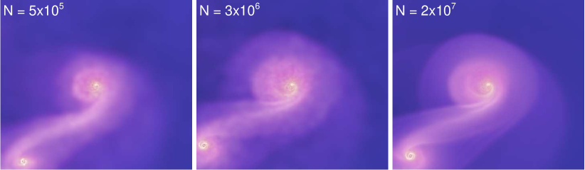
We have performed a series of analogous resolution tests on our intermediate (Table 2) and small-scale simulations (Table 3), covering a similar span in particle number. For the intermediate-scale simulations, we have varied the SPH smoothing length and gravitational softening length from $<1\,$pc to $\sim 10\,$pc. We find that the results of particular importance for this paper, e.g., the total gas mass that loses angular momentum and flows to smaller scales, are well-converged for all the resolutions $\lesssim 10\,$pc used here. This is not surprising, because for physical reasons (discussed in the main text), the material reaches an angular momentum barrier at $\sim 10\,$pc. For our small-scale simulations, we find similar behavior for all force resolutions $\ll 1\,$pc (experimenting with a range of softenings from $0.02-1\,$pc), and with good convergence at higher particle numbers $\gtrsim$ a few $10^{5}$. Given the range of resolution explored, comparison with Figure 10 demonstrates that, especially in our high-resolution studies, even the verticle structure of the gaseous disks is well-resolved (in the highest-resolution cases, the typical $h_{\rm sml}/R<0.01$). Figure 15 shows an example resolution test varying from $5\times 10^{5}-2\times 10^{7}$ particles.

Figure 16: Simulations testing the effects of large-scale tidal forces in our re-simulations. Left: Re-simulation of the central $\sim 10\,$pc-kpc of a larger-scale galaxy merger simulation, in which the full time-dependent potential from the large-scale simulation is analytically included in the re-simulation. We show the gas density and star formation rate density as in Figure 3, three large-scale dynamical times after the beginning of the simulation. Center: Same re-simulation, but without the additional potential from the large-scale material; i.e., the gravitational potential is only from the “live” material being re-simulated in the central kpc. The image is at the same point in time. Right: Gas density profiles of both re-simulations at the peak of the resulting inflows. Because the density declines rapidly with radius, the large-scale density/potential fields make no significant difference to the dynamics at the these scales.

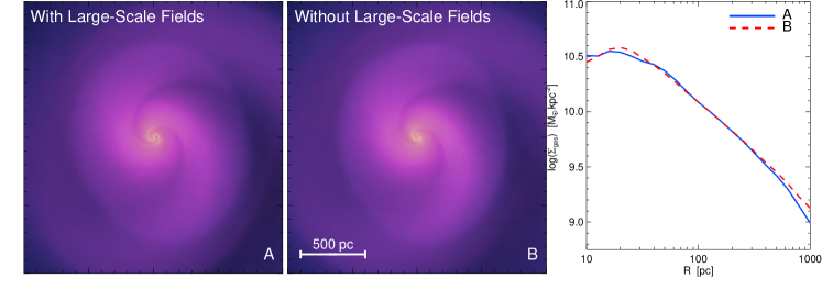
A.2 Do the Results Depend on Large-scale Tidal Fields?

Because we are simulating the properties of large-scale non-axisymmetric systems, one might worry that the tidal forces from large radii could be important. This is certainly the case, e.g., in cosmological simulations. In the present context, the question is whether we need to include the matter distribution at $\sim 10\,$kpc in real-time to understand the dynamics of material at $\lesssim 100\,$pc.

We assess this directly as follows. For a given re-simulation of the nuclear regions, we determine the matter distribution of the larger-scale simulation from which the re-simulation is drawn and analytically fit the non-axisymmetric contributions to the potential at all radii. Figure 16 compares the results from a re-simulation in which we include the large-scale non-axisymmetric potential at $\gtrsim$ kpc with our standard approach, in which we do not include this potential and in which the matter at large radii is not included in the re-simulation (so the information is lost). This is simulation If9b5 in Table 2, a $\sim 0.01-1$ kpc re-simulation of the galactic nucleus during a galaxy-galaxy merger simulation at the peak of nuclear activity, just after the coalescence of the two galactic nuclei. At large scales, tidal tails are still present (these will take up to several Gyr to fully relax), and the system is largely unrelaxed outside of a few hundred pc, so this is a time when the large-scale effects would a priori be the most important. In the simulations shown in Figure 16 (left panel), we analytically fit the large-scale tidal field in the galaxy-galaxy merger simulation at multiple times, and interpolate it in time in our re-simulation.

Figure 16 shows that there is effectively no difference between the simulations with and without the large-scale tidal field, at any of the radii of interest. Including large-scale tidal forces does somewhat truncate the large spiral wave pattern that appears as a secondary instability in the intermediate-scale simulation, but this truncation occurs only on the largest radii $\gtrsim 500\,$pc, radii that we are not trying to model in detail in the re-simulation. Most importantly, the scales which the re-simulation is intended to accurately represent, $\lesssim 100\,$pc, are indistinguishable in the two simulations. The reason for this is ultimately that the mass profile is a relatively steep function of radius. If a mass $\delta M$ is enclosed in an annulus at a radius $r$, then the tidal force it produces is $\propto|a|\delta M/r^{3}$, where $|a|$ is the magnitude of the non-axisymmetric component of the mass distribution at that annulus. The contribution of a given large radius to the tidal force at small radii is thus $\propto\rho(r)$, the local mass density. This, however, is always a decreasing function of (increasing) radius, so that material at larger radii makes little contribution to the tidal force. This can be compared with the role of tidal forces in determining the angular momentum of large-scale dark matter structures and ultimately (via these structures) dark matter halos; since the large-scale matter field has $\rho\sim$constant on average, there are significant contributions to tidal forces from all radii. This is why including the information about large-scale tidal fields is critical for simulations of cooling and galaxy formation, but it is not important when following the further inflows of material in individual galaxies.

We have performed similar experiments to those shown here for other intermediate-scale simulations (both in mergers and isolated galaxies), and for our smallest-scale simulations ($\sim 0.1-10\,$pc), and reach the same conclusions in each case.

A.3 Do the Results Depend on Initial Conditions?

A reasonable question about our re-simulation technique is whether it might be sensitive to the precise initial conditions in the nuclear disk that is initialized at high resolution. In particular, there is little detailed information about the structure or dynamics of the nuclear disk in the original larger-scale simulation, precisely because it lacked the necessary resolution to study the small-scale nuclear dynamics. Here we show that our results do not depend on the details of how we initialize the re-simulations in the nuclear region. The fundamental reason for this is that the nuclear dynamics is governed by instabilities that are self-consistently generated on small scales. These instabilities depend primarily on the gross structural properties of the nucleus, and rapidly lose memory of the initial conditions.

Figure 17: Effects of initial conditions on our re-simulations of galactic nuclei. Panels A-E show the gas density and star formation rate density $10^{8}$ yr after the beginning of the simulation. Bottom right: Surface density profiles of all five simulations at the same time. A: Re-simulation of the central $\sim$kpc from a larger-scale merger simulation (as in Figure 16). The initial conditions are taken exactly from the larger-scale simulation, i.e., with inherited non-axisymmetric modes. B: Same as A but in this case we initialize azimuthally averaged (i.e., axisymmetric) profiles. C: Even more idealized: we initialize an axisymmetric bulge+disk+halo+BH system with analytic profile shapes; the mass and radius of each component is the same as that of the material in the original large-scale simulation at these radii, but the profile shapes are not. D: Same as A, but with random seed non-axisymmetric modes having order unity random amplitudes and phases E: Same as A, but the gas at $\lesssim 100\,$pc is removed so that there is initially a central “hole” in the gas distribution. Comparison of A-E demonstrates that the precise initial conditions have little effect on the mode dynamics and gas transport. Morphologically, systems with stronger (weaker) initial seeds develop modes slightly more quickly (slowly), but this time shift has little significant or lasting effect on the dynamics.

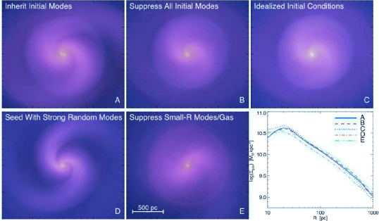
Figure 17 shows the results of five different re-simulations, each with different initial conditions. These are all $\sim 100\,$pc re-simulations of the central regions from a galaxy-merger simulation (intermediate-scale simulation If9b5 in Table 2), just after the coalescence of the two galaxy nuclei. Panel A is a rigorous re-simulation of the matter distribution in the central kpc of the large-scale simulation, with the matter initialized “as-is” from the large-scale simulation. Panel B is the same except we do not include any of the non-axisymmetric modes in the density, pressure, potential, etc. in the initial conditions; i.e., we azimuthally average the initial conditions used in Panel A. Panel C is even more idealized: the system is axisymmetric and with exponential disk and Hernquist profiles for the “disky” and “spherical” components in the re-simulation, respectively. The masses and effective radii of these components match the original simulation, but the profiles are these simple analytic approximations rather than the true profile from the larger-scale simulation. To test whether the presence of particular non-axisymmetries is important, Panel D includes non-axisymmetric structure in the initial conditions, but the precise modes are randomly chosen in phase and amplitude and so do not match the actual non-axisymmetries from Panel A. Finally, all of the above simulations include gas at small radii in the initial conditions; this is because the finite smoothing length in the larger-scale simulation spreads gas out over a region $\sim 100$ pc even though the dynamics below this scale is completely incorrect. In order to be as conservative as possible, Panel E considers an initial “hole” in the gas distribution at radii that are not resolved in the large scale simulation; for numerical reasons, the “hole” is a sharp power-law cutoff inside $100\,$pc. This could represent a very hard angular momentum barrier, such as a strong inner Linblad resonance.

The images and surface density plots in Figure 17 are $10^{8}$ yr after the beginning of the simulation. There is remarkably little difference in the mode structure visible in the images. More quantitatively, the surface density profiles are very similar, with significant gas inflow to $\sim 10$ pc. This demonstrates that the precise initial conditions used in the re-simulations are not important for most of our results. The fundamental reason for this is that the instabilities that dominate the dynamics arise from the internal structure of the material; they depend on the mass and scale-lengths of the rotationally and dispersion supported components, but not on the initial seed amplitudes of various modes. In the case of axisymmetric initial conditions (Panel B), the initial perturbations take slightly longer to appear because the initial power present to be amplified is smaller (it is due to particle noise); and in the case of strong initial modes (Panel D), the instability is slightly more developed at the fixed time shown here. However, these time shifts have little long-term effect on the evolution of the system.

Figure 18: Illustration of one of our ultra-high resolution simulations (Inf28b2h). The gas density distribution is shown face-on, as in Figure 17, in most panels, and edge-on at bottom right. The initial conditions are those of a typical intermediate-scale re-simulation, but with $\sim 10^{7}$ particles and sub-pc resolution. This obviates the need for a secondary “re-simulation” of the nuclear scales. The large-scale modes fuel gas inwards and here lead to a large nuclear gas mass, which then forms a lopsided $m=1$ mode around the BH and drives further inflow. The eccentric nuclear gas disk is clearly visible, and similar to those in our nuclear-scale re-simulations; in fact there is no statistical difference, given similar boundary conditions.

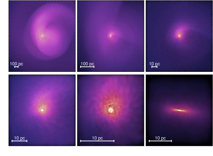
The robustness of our conclusions to resolution, tidal fields, and initial conditions is also demonstrated by the fact that our ultra-high resolution simulations, discussed at length in the text, give identical results to our standard re-simulated runs. These ultra-high resolution simulations allow us to bridge the boundaries of our standard re-simulations, and so do not suffer the potential negative effects considered here. Figure 18 shows an illustrative example of one such simulation about mid-way through the period of peak activity. The simulation is initialized as one of our typical intermediate-scale re-simulations, but with $\sim 10^{7}$ particles, giving a final resolution of $\lesssim$ pc. On large scales, the dynamics is similar to our other intermediate-scale runs, with an $m=2$ mode forming rapidly (there are non-trivial mode amplitudes from $m=1-3$). The inflow leads to large gas masses at small radii; by the active phase shown in Figure 18, the lopsided, eccentric nuclear disk is evident. The properties of this disk are statistically indistinguishable from those in our nuclear-scale re-simulations, given similar boundary conditions (compare e.g. Figure 2).

Appendix B ISM Physics

Figure 19: Examples of the problems that occur if systems are evolved without some “feedback” to prevent runaway cooling and fragmentation. Top Left: Gas density in such an initially smooth re-simulation of the central $\sim$kpc (unlike in the main text, here darker areas represent higher-density to highlight the fragmentation). The system here can cool to $10^{4}\,$K and has no feedback ($q_{\rm eos}=0$); the image is shown after $\sim 2\times 10^{6}$ years (less than the global dynamical time). Top Right: The same initial conditions but for our fiducial model – a moderate subgrid (“turbulent”) sound speed $\sim 30\,{\rm km\,s^{-1}}$ ($q_{\rm eos}=0.125$) in dense star-forming regions. In the no feedback $q_{\rm eos}=0$ case, gas clumps at the Jeans scale and rapidly turns into stars – leading to a severe violation of the observed global Kennicutt (1998) relation. Bottom Left: Stellar density profiles after $10^{7}\,$yr, for simulations with no feedback (two examples shown, with different cooling floors as labeled) and our fiducial $q_{\rm eos}=0.125$ model; the initial density is just $10^{10}\,M_{\sun}\,{\rm kpc^{-2}}$ at small radii. We also show the observed stellar mass density profiles of massive cusp ellipticals in Virgo from Kormendy et al. (2009), chosen to have the same mass at $>0.5-1\,$kpc. In the absence of feedback, runaway fragmentation and the inability of clumps to dissolve inevitably leads to the formation of an extremely massive nuclear stellar cluster with a mass and surface density at least an order of magnitude larger than any observed. Bottom Right: The accretion rate into the central $10\,$pc for both gas (dotted) and already-formed stars (solid). In the $q_{\rm eos}=0$ models, sinking clumps provide large gas accretion rates $\sim 10-100\,M_{\sun}\,{\rm yr^{-1}}$, but the stellar inflow rate typically exceeds the gas inflow rate by a factor of $\sim 10$; this is inconsistent with the observed stellar densities at small radii. Our fiducial, moderate-feedback case, by contrast, drives primarily gas – not stars – to small radii.

Figure 20: Effects of varying the assumed efficiency of stellar feedback on the resulting nuclear eccentric disk, given identical inflow conditions at $100\,$pc. We show the gas surface density with color indicating specific SFR (as Figure 17), for several choices of $q_{\rm eos}$ (from the survey Nf8h2b4q). The range shown corresponds to sub-grid turbulent velocities ranging from $\sim 20-100\,{\rm km\,s^{-1}}$ in the high star-formation rate regions of the ISM. The efficiency of feedback affects the level of substructure. However, the general character and appearance of the lopsided disk mode is similar over the entire plausible range. Provided the catastrophic fragmentation in Figure 19 can be avoided, our qualitative conclusions are independent of $q_{\rm eos}$.

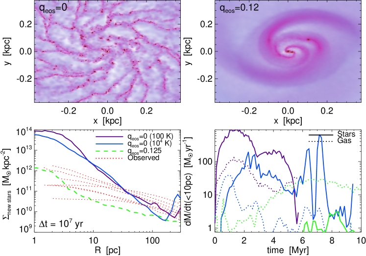
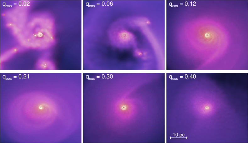
As discussed extensively in §2 & §7, the largest a priori uncertainty in our modeling is the question of what physics should be included to describe the behavior of the ISM. Our approach is to include a large “turbulent” sound speed in the equation state, as a subgrid model for the effects of feedback by stellar winds, radiation pressure, and supernovae on the ISM. We choose the turbulent velocity largely by comparison to observed systems (Fig. 1). The resulting turbulent velocities $\sim 30-100\ {\rm km\,s^{-1}}$ are also reasonably consistent with theoretical estimates of the feedback required to maintain $Q\sim 1$ and disrupt molecular clouds in starburst environments (Thompson et al., 2005; Murray et al., 2009).

To illustrate the importance of including a subgrid model, in this Appendix we compare the results of our standard models with a simulation in which the ISM is isothermal at $\sim 10^{4}$ K, i.e., $c_{s}\simeq 10\ {\rm km\,s^{-1}}$ ($q_{\rm eos}=0$). We have experimented with a range of isothermal cooling floors from $c_{s}=1-15\,{\rm km\,s^{-1}}$ ($100-3\times 10^{4}\,$K), but the results here are generic to this range. Figure 19 shows several of the key results comparing the $c_{s}\simeq 10\ {\rm km\,s^{-1}}$ simulation with our fiducial $q_{\rm eos}=0.125$ simulation, for a re-simulation on $\sim 100\,$pc scales. From the images it is clear that after just a few local dynamical times in the intermediate-scale disk, the simulation without feedback has violently fragmented into large clumps. It is important to stress that in this simulation we fully resolve the Jeans and Toomre lengths so the fragmentation is physical, not numerical.

The difficulty with the $c_{s}\simeq 10\ {\rm km\,s^{-1}}$ ($q_{\rm eos}=0$) simulation is that, absent a full model for how feedback can either suppress their formation or suppress their internal star formation, the only possibility is that the clumps “run away” and turn efficiently into stars. The runaway and final consequences of the fragmentation for star formation and the IMF are sensitive to details of the cooling rates and cooling function, but the end result of runaway star formation is inevitable if the gas is allowed to be arbitrarily cold and has a small cooling time (Gammie, 2001; Nayakshin et al., 2007; Thompson et al., 2005). This has several dramatic effects. First, the global star formation efficiency is significantly enhanced – for the same mean gas surface density, most of the gas will turn into stars in $\sim 1-4$  local dynamical times absent feedback. This is a factor of $10-50$ higher than implied by the Schmidt-Kennicutt laws. For comparison, our fiducial $q_{\rm eos}=0.125$ simulation has a star formation efficiency per dynamical time of a few percent, much more consistent with observations. Because of the rapid and efficient star formation in the $c_{s}=10\ {\rm km\,s^{-1}}$ simulation, the clumps quickly convert a large fraction of their mass to stars; the resulting massive stellar clusters sink and coalesce via clump-clump scattering and/or dynamical friction, to the center of the galaxy. As the lower-right panel of Figure 19 shows, most of the mass flowing into the central $\sim 10$ pc in the $c_{s}\simeq 10\ {\rm km\,s^{-1}}$ simulation is in the form of stars, rather than gas. This results in the formation of an extremely massive nuclear star cluster, with a mass of $\sim 10^{9}\,M_{\sun}$ inside the central $\sim 10-20\,$pc – a factor of at least $\sim 10\,$ larger than observed nuclear star clusters (Böker et al., 2004; Côté et al., 2006; Ferrarese et al., 2006a). Indeed, the resulting stellar surface density at small scales (left panel of Fig. 19) significantly exceeds the highest nuclear densities observed in any cusp ellipticals (Ferrarese et al., 2006b; Kormendy et al., 2009; Lauer et al., 2007), or for that matter any nuclear star clusters, globular clusters, nuclear disks, or other high-density stellar systems (Hopkins et al., 2009e).

In contrast to the constant $c_{s}\simeq 10\ {\rm km\,s^{-1}}$ simulation, our fiducial simulation with significant subgrid feedback does not clump up into many dense star clusters. This is also not completely physical since in reality we expect that the ISM should have significant sub-structure on the scales we model (including, e.g., molecular clouds and star clusters). However, when such self-gravitating gaseous clumps form, observations strongly suggest that are likely to be short-lived and/or to inefficiently form stars. Our subgrid model assumes that most of the mass remains in a diffuse ISM, rather than becoming bound in dense star clusters. Not only is the latter physically implausible, but Figure 19 demonstrates that it strongly violates observational constraints. Note that there are conditions under which even an extremely cold gaseous disk could avoid catastrophic fragmentation (see e.g. Lodato & Rice, 2004; Rice et al., 2005; Boley et al., 2006; Krumholz et al., 2007), particularly the case in which the cooling time is sufficiently long such that continued cooling is offset by gravitational heating (giving rise to sustained local structure such as tightly-wound spiral arms, but not runaway fragmentation). However, the cooling rates under typical conditions in our simulations are much too rapid to reach this regime; we could, of course, modify the cooling function to suppress the cooling rate and/or mimic some continuous heating term – but this is effectively equivalent to adopting a new sub-grid feedback/microphysics model, and we find it has the same qualitative effects.

Figure 20 shows the effects of varying the efficiency of feedback from supernovae and massive stars, encapsulated in the parameter $q_{\rm eos}$. Specifically, we show results of a set of nuclear scale simulations (Nf8h2b4q in Table 3) having $q_{\rm eos}=0.02-0.40$ (effective turbulent velocities $\sim 20-100\,{\rm km\,s^{-1}}$), roughly the lower and upper limits allowed by observational constraints for the systems of interest in Figure 1. Figure 20 shows that the choice of sub-resolution model has a significant effect on the amount of resolved sub-structure in the simulation. This is not surprising since larger turbulent velocities raise the Jeans mass/length, above which gravity is the dominant force. The key point, however, is that all of the simulations show a similar nuclear lopsided disk. In terms of the properties of inflow and global instability discussed throughout this paper, the differences produced by changing $q_{\rm eos}$ are similar to the differences produced by somewhat different galaxy properties. The fundamental reason for the weak dependence on the subgrid model is that the torques in our simulations are primarily determined by gravity, not hydrodynamic forces or viscosity. The primary role of the subgrid feedback model is simply to prevent catastrophic fragmentation of the galactic gas. Provided this can be accomplished, our qualitative conclusions do not depend on the details of the feedback model.

References

- Adams et al. (1989) Adams, F. C., Ruden, S. P., & Shu, F. H. 1989, ApJ, 347, 959
- Allen et al. (2007) Allen, L., et al. 2007, in Protostars and Planets V, ed. B. Reipurth, D. Jewitt, & K. Keil, 361–376
- Aller & Richstone (2007) Aller, M. C., & Richstone, D. O. 2007, ApJ, 665, 120
- Aoki et al. (1979) Aoki, S., Noguchi, M., & Iye, M. 1979, PASJ, 31, 737
- Athanassoula (2008) Athanassoula, E. 2008, MNRAS, 390, L69
- Athanassoula et al. (1983) Athanassoula, E., Bienayme, O., Martinet, L., & Pfenniger, D. 1983, A&A, 127, 349
- Athanassoula et al. (2005) Athanassoula, E., Lambert, J. C., & Dehnen, W. 2005, MNRAS, 363, 496
- Balbus & Hawley (1998) Balbus, S. A., & Hawley, J. F. 1998, Reviews of Modern Physics, 70, 1
- Banerjee et al. (2004) Banerjee, R., Pudritz, R. E., & Holmes, L. 2004, MNRAS, 355, 248
- Bardeen (1975) Bardeen, J. M. 1975, in IAU Symposium, Vol. 69, Dynamics of the Solar Systems, ed. A. Hayli, 297–+
- Barnes (1998) Barnes, J. E. 1998, in Saas-Fee Advanced Course 26: Galaxies: Interactions and Induced Star Formation; Springer-Verlag Berlin/Heidelberg, ed. R. C. Kennicutt, Jr., F. Schweizer, J. E. Barnes, D. Friedli, L. Martinet, & D. Pfenniger, 275–+
- Barnes & Hernquist (1996) Barnes, J. E., & Hernquist, L. 1996, ApJ, 471, 115
- Barnes & Hernquist (1991) Barnes, J. E., & Hernquist, L. E. 1991, ApJL, 370, L65
- Begelman & Shlosman (2009) Begelman, M., & Shlosman, I. 2009, ApJL, in press, arXiv:0904.4247, 0904, 4247
- Bell & de Jong (2001) Bell, E. F., & de Jong, R. S. 2001, ApJ, 550, 212
- Bender et al. (2005) Bender, R., et al. 2005, ApJ, 631, 280
- Berentzen et al. (2007) Berentzen, I., Shlosman, I., Martinez-Valpuesta, I., & Heller, C. H. 2007, ApJ, 666, 189
- Bigiel et al. (2008) Bigiel, F., Leroy, A., Walter, F., Brinks, E., de Blok, W. J. G., Madore, B., & Thornley, M. D. 2008, AJ, 136, 2846
- Blitz (1993) Blitz, L. 1993, in Protostars and Planets III (University of Arizona Press: Tucson), ed. E. H. Levy & J. I. Lunine, 125–161
- Block et al. (2001) Block, D. L., Puerari, I., Knapen, J. H., Elmegreen, B. G., Buta, R., Stedman, S., & Elmegreen, D. M. 2001, Astronomy and Astrophysics, 375, 761
- Böker et al. (2004) Böker, T., Sarzi, M., McLaughlin, D. E., van der Marel, R. P., Rix, H.-W., Ho, L. C., & Shields, J. C. 2004, AJ, 127, 105
- Boley et al. (2006) Boley, A. C., Mejía, A. C., Durisen, R. H., Cai, K., Pickett, M. K., & D’Alessio, P. 2006, ApJ, 651, 517
- Bonnell et al. (2006) Bonnell, I. A., Dobbs, C. L., Robitaille, T. P., & Pringle, J. E. 2006, MNRAS, 365, 37
- Bouché et al. (2007) Bouché, N., et al. 2007, ApJ, 671, 303
- Bournaud & Combes (2002) Bournaud, F., & Combes, F. 2002, A&A, 392, 83
- Bournaud et al. (2005) Bournaud, F., Combes, F., Jog, C. J., & Puerari, I. 2005, A&A, 438, 507
- Bryant & Scoville (1999) Bryant, P. M., & Scoville, N. Z. 1999, AJ, 117, 2632
- Bullock et al. (2001) Bullock, J. S., et al. 2001, MNRAS, 321, 559
- Cai et al. (2008) Cai, K., Durisen, R. H., Boley, A. C., Pickett, M. K., & Mejía, A. C. 2008, ApJ, 673, 1138
- Carlberg (1986) Carlberg, R. G. 1986, ApJ, 310, 593
- Chang et al. (2007) Chang, P., Murray-Clay, R., Chiang, E., & Quataert, E. 2007, The Astrophysical Journal, 668, 236
- Christodoulou et al. (1995) Christodoulou, D. M., Shlosman, I., & Tohline, J. E. 1995, ApJ, 443, 551
- Cossins et al. (2009) Cossins, P., Lodato, G., & Clarke, C. J. 2009, MNRAS, 393, 1157
- Côté et al. (2006) Côté, P., et al. 2006, ApJS, 165, 57
- Covington et al. (2008) Covington, M., Dekel, A., Cox, T. J., Jonsson, P., & Primack, J. R. 2008, MNRAS, 384, 94
- Cox et al. (2006) Cox, T. J., Dutta, S. N., Di Matteo, T., Hernquist, L., Hopkins, P. F., Robertson, B., & Springel, V. 2006, ApJ, 650, 791
- Cuadra et al. (2009) Cuadra, J., Armitage, P. J., Alexander, R. D., & Begelman, M. C. 2009, Monthly Notices of the Royal Astronomical Society, 393, 1423
- Dasyra et al. (2006) Dasyra, K. M., et al. 2006, ApJ, 638, 745
- Dasyra et al. (2007) —. 2007, ApJ, 657, 102
- Davies et al. (2007) Davies, R. I., Sánchez, F. M., Genzel, R., Tacconi, L. J., Hicks, E. K. S., Friedrich, S., & Sternberg, A. 2007, ApJ, 671, 1388
- Debattista et al. (2006) Debattista, V. P., Ferreras, I., Pasquali, A., Seth, A., De Rijcke, S., & Morelli, L. 2006, ApJL, 651, L97
- DeBuhr et al. (2009) DeBuhr, J., Quataert, E., Ma, C.-P., & Hopkins, P. 2009, MNRAS, in press, arXiv:0909.2872
- Di Matteo et al. (2005) Di Matteo, T., Springel, V., & Hernquist, L. 2005, Nature, 433, 604
- Dotti et al. (2009) Dotti, M., Ruszkowski, M., Paredi, L., Colpi, M., Volonteri, M., & Haardt, F. 2009, MNRAS, 396, 1640
- Downes & Solomon (1998) Downes, D., & Solomon, P. M. 1998, ApJ, 507, 615
- Dubinski et al. (2009) Dubinski, J., Berentzen, I., & Shlosman, I. 2009, ApJ, 697, 293
- Durbala et al. (2009) Durbala, A., Buta, R., Sulentic, J. W., & Verdes-Montenegro, L. 2009, MNRAS, in press [arXiv:0905.2340]
- Earn & Sellwood (1995) Earn, D. J. D., & Sellwood, J. A. 1995, ApJ, 451, 533
- Elmegreen (2007) Elmegreen, B. G. 2007, ApJ, 668, 1064
- Escala (2007) Escala, A. 2007, ApJ, 671, 1264
- Escala et al. (2004) Escala, A., Larson, R. B., Coppi, P. S., & Mardones, D. 2004, ApJ, 607, 765
- Evans et al. (2006) Evans, A. S., Solomon, P. M., Tacconi, L. J., Vavilkin, T., & Downes, D. 2006, AJ, 132, 2398
- Ferrarese & Merritt (2000) Ferrarese, L., & Merritt, D. 2000, ApJL, 539, L9
- Ferrarese et al. (2006a) Ferrarese, L., et al. 2006a, ApJL, 644, L21
- Ferrarese et al. (2006b) —. 2006b, ApJS, 164, 334
- Förster Schreiber et al. (2006) Förster Schreiber, N. M., et al. 2006, ApJ, 645, 1062
- Gammie (2001) Gammie, C. F. 2001, ApJ, 553, 174
- García-Burillo et al. (2005) García-Burillo, S., Combes, F., Schinnerer, E., Boone, F., & Hunt, L. K. 2005, Astronomy and Astrophysics, 441, 1011
- Gebhardt et al. (2000) Gebhardt, K., et al. 2000, ApJL, 539, L13
- Goodman (2003) Goodman, J. 2003, MNRAS, 339, 937
- Greene et al. (2009) Greene, J. E., Zakamska, N. L., Liu, X., Barth, A. J., & Ho, L. C. 2009, ApJ, in press, arXiv:0907.1086
- Gunn (1987) Gunn, J. E. 1987, in Nearly Normal Galaxies. From the Planck Time to the Present (New York: Springer-Verlag), ed. S. M. Faber, 455–464
- Haan et al. (2009) Haan, S., Schinnerer, E., Emsellem, E., García-Burillo, S., Combes, F., Mundell, C. G., & Rix, H.-W. 2009, The Astrophysical Journal, 692, 1623
- Heller et al. (2001) Heller, C., Shlosman, I., & Englmaier, P. 2001, The Astrophysical Journal, 553, 661
- Hernquist (1989) Hernquist, L. 1989, Nature, 340, 687
- Hernquist (1990) —. 1990, ApJ, 356, 359
- Hernquist (1993) —. 1993, ApJ, 404, 717
- Hernquist & Ostriker (1992) Hernquist, L., & Ostriker, J. P. 1992, Astrophysical Journal, 386, 375
- Hernquist et al. (1993) Hernquist, L., Spergel, D. N., & Heyl, J. S. 1993, ApJ, 416, 415
- Hibbard & Yun (1999) Hibbard, J. E., & Yun, M. S. 1999, ApJL, 522, L93
- Hicks et al. (2009) Hicks, E. K. S., Davies, R. I., Malkan, M. A., Genzel, R., Tacconi, L. J., Sánchez, F. M., & Sternberg, A. 2009, ApJ, 696, 448
- Ho (2005) Ho, L. C. 2005, ApJ, 629, 680
- Hopkins et al. (2009a) Hopkins, P. F., Cox, T. J., Dutta, S. N., Hernquist, L., Kormendy, J., & Lauer, T. R. 2009a, ApJS, 181, 135
- Hopkins et al. (2008a) Hopkins, P. F., Cox, T. J., & Hernquist, L. 2008a, ApJ, 689, 17
- Hopkins et al. (2009b) Hopkins, P. F., Cox, T. J., Younger, J. D., & Hernquist, L. 2009b, ApJ, 691, 1168
- Hopkins & Hernquist (2006) Hopkins, P. F., & Hernquist, L. 2006, ApJS, 166, 1
- Hopkins & Hernquist (2009) —. 2009, MNRAS, in press, arXiv:0910.4582
- Hopkins et al. (2008b) Hopkins, P. F., Hernquist, L., Cox, T. J., Dutta, S. N., & Rothberg, B. 2008b, ApJ, 679, 156
- Hopkins et al. (2009c) Hopkins, P. F., Hernquist, L., Cox, T. J., Kereš, D., & Wuyts, S. 2009c, ApJ, 691, 1424
- Hopkins et al. (2007) Hopkins, P. F., Hernquist, L., Cox, T. J., Robertson, B., & Krause, E. 2007, ApJ, 669, 67
- Hopkins et al. (2005) Hopkins, P. F., Hernquist, L., Martini, P., Cox, T. J., Robertson, B., Di Matteo, T., & Springel, V. 2005, ApJL, 625, L71
- Hopkins et al. (2009d) Hopkins, P. F., Lauer, T. R., Cox, T. J., Hernquist, L., & Kormendy, J. 2009d, ApJS, 181, 486
- Hopkins et al. (2009e) Hopkins, P. F., Murray, N., Quataert, E., & Thompson, T. A. 2009e, MNRAS, in press, arXiv:0908.4088
- Hopkins & Quataert (2010) Hopkins, P. F., & Quataert, E. 2010, MNRAS, L62+
- Hopkins et al. (2009f) Hopkins, P. F., Somerville, R. S., Cox, T. J., Hernquist, L., Jogee, S., Kereš, D., Ma, C.-P., Robertson, B., & Stewart, K. 2009f, MNRAS, 397, 802
- Imanishi (2002) Imanishi, M. 2002, ApJ, 569, 44
- Imanishi (2003) —. 2003, ApJ, 599, 918
- Imanishi & Wada (2004) Imanishi, M., & Wada, K. 2004, ApJ, 617, 214
- Iono et al. (2007) Iono, D., et al. 2007, ApJ, 659, 283
- Jogee (2006) Jogee, S. 2006, in Lecture Notes in Physics, Berlin Springer Verlag, Vol. 693, Physics of Active Galactic Nuclei at all Scales, ed. D. Alloin, 143–+
- Jogee et al. (2005) Jogee, S., Scoville, N., & Kenney, J. D. P. 2005, ApJ, 630, 837
- Johansson et al. (2009a) Johansson, P. H., Naab, T., & Burkert, A. 2009a, ApJ, 690, 802
- Johansson et al. (2009b) —. 2009b, ApJL, in press, arXiv:0910.2232
- Kalnajs (1971) Kalnajs, A. J. 1971, ApJ, 166, 275
- Kauffmann et al. (2003) Kauffmann, G., et al. 2003, MNRAS, 346, 1055
- Kawakatu & Wada (2008) Kawakatu, N., & Wada, K. 2008, ApJ, 681, 73
- Kennicutt (1998) Kennicutt, Jr., R. C. 1998, ApJ, 498, 541
- Kennicutt et al. (2007) Kennicutt, Jr., R. C., et al. 2007, ApJ, 671, 333
- Kewley et al. (2006) Kewley, L. J., Groves, B., Kauffmann, G., & Heckman, T. 2006, MNRAS, 372, 961
- Kim et al. (2006) Kim, M., Ho, L. C., & Im, M. 2006, ApJ, 642, 702
- Knapen et al. (2002) Knapen, J. H., Pérez-Ramírez, D., & Laine, S. 2002, Monthly Notice of the Royal Astronomical Society, 337, 808
- Knapen et al. (2000) Knapen, J. H., Shlosman, I., & Peletier, R. F. 2000, ApJ, 529, 93
- Kondratko et al. (2005) Kondratko, P. T., Greenhill, L. J., & Moran, J. M. 2005, ApJ, 618, 618
- Kormendy (1989) Kormendy, J. 1989, ApJL, 342, L63
- Kormendy et al. (2009) Kormendy, J., Fisher, D. B., Cornell, M. E., & Bender, R. 2009, ApJS, 182, 216
- Kormendy & Freeman (2004) Kormendy, J., & Freeman, K. C. 2004, in IAU Symposium, Vol. 220, Dark Matter in Galaxies, ed. S. Ryder, D. Pisano, M. Walker, & K. Freeman, 377–+
- Kormendy & Richstone (1995) Kormendy, J., & Richstone, D. 1995, ARA&A, 33, 581
- Krips et al. (2007) Krips, M., et al. 2007, A&A, 468, L63
- Krumholz et al. (2007) Krumholz, M. R., Klein, R. I., & McKee, C. F. 2007, ApJ, 656, 959
- Krumholz et al. (2006) Krumholz, M. R., Matzner, C. D., & McKee, C. F. 2006, ApJ, 653, 361
- Krumholz & McKee (2005) Krumholz, M. R., & McKee, C. F. 2005, ApJ, 630, 250
- Krumholz & Tan (2007) Krumholz, M. R., & Tan, J. C. 2007, ApJ, 654, 304
- Laine et al. (2002) Laine, S., Shlosman, I., Knapen, J. H., & Peletier, R. F. 2002, The Astrophysical Journal, 567, 97
- Laine et al. (2003) Laine, S., van der Marel, R. P., Rossa, J., Hibbard, J. E., Mihos, J. C., Böker, T., & Zabludoff, A. I. 2003, AJ, 126, 2717
- Larson (1981) Larson, R. B. 1981, MNRAS, 194, 809
- Larson (2009) —. 2009, Nature, in press, arXiv:0909.3110
- Lau & Bertin (1978) Lau, Y. Y., & Bertin, G. 1978, ApJ, 226, 508
- Lauer et al. (1993) Lauer, T. R., et al. 1993, AJ, 106, 1436
- Lauer et al. (1996) —. 1996, ApJL, 471, L79+
- Lauer et al. (2007) —. 2007, ApJ, 664, 226
- Lemoine-Busserolle et al. (2009) Lemoine-Busserolle, M., Bunker, A., Lamareille, F., & Kissler-Patig, M. 2009, MNRAS, in press, arXiv:0909.1386
- Levine et al. (2008) Levine, R., Gnedin, N. Y., Hamilton, A. J. S., & Kravtsov, A. V. 2008, ApJ, 678, 154
- Lodato & Rice (2004) Lodato, G., & Rice, W. K. M. 2004, MNRAS, 351, 630
- Lynden-Bell & Kalnajs (1972) Lynden-Bell, D., & Kalnajs, A. J. 1972, MNRAS, 157, 1
- Magorrian et al. (1998) Magorrian, J., et al. 1998, AJ, 115, 2285
- Mandelbaum et al. (2006) Mandelbaum, R., Seljak, U., Kauffmann, G., Hirata, C. M., & Brinkmann, J. 2006, MNRAS, 368, 715
- Martini (2004) Martini, P. 2004, in Coevolution of Black Holes and Galaxies (Cambridge: Cambridge University Press), ed. L. C. Ho, 169
- Martini & Pogge (1999) Martini, P., & Pogge, R. W. 1999, Astron. J., 118, 2646
- Martini et al. (2003) Martini, P., Regan, M. W., Mulchaey, J. S., & Pogge, R. W. 2003, ApJ, 589, 774
- Mayer et al. (2007) Mayer, L., Kazantzidis, S., Madau, P., Colpi, M., Quinn, T., & Wadsley, J. 2007, Science, 316, 1874
- McKee & Ostriker (1977) McKee, C. F., & Ostriker, J. P. 1977, ApJ, 218, 148
- Mihos & Hernquist (1994) Mihos, J. C., & Hernquist, L. 1994, ApJL, 431, L9
- Mihos & Hernquist (1996) —. 1996, ApJ, 464, 641
- Murray et al. (2009) Murray, N., Quataert, E., & Thompson, T. A. 2009, ApJ, in press [arXiv:0906.5358]
- Narayan et al. (1987) Narayan, R., Goldreich, P., & Goodman, J. 1987, MNRAS, 228, 1
- Nayakshin et al. (2007) Nayakshin, S., Cuadra, J., & Springel, V. 2007, MNRAS, 379, 21
- Nayakshin & King (2007) Nayakshin, S., & King, A. 2007, MNRAS, in press, arXiv:0705.1686
- Noguchi (1988) Noguchi, M. 1988, A&A, 203, 259
- O’Shea et al. (2005) O’Shea, B. W., Nagamine, K., Springel, V., Hernquist, L., & Norman, M. L. 2005, ApJS, 160, 1
- Ostriker et al. (1992) Ostriker, E. C., Shu, F. H., & Adams, F. C. 1992, ApJ, 399, 192
- Ostriker (1980) Ostriker, J. P. 1980, Comments on Astrophysics, 8, 177
- Peiris & Tremaine (2003) Peiris, H. V., & Tremaine, S. 2003, ApJ, 599, 237
- Peletier et al. (1999) Peletier, R. F., et al. 1999, ApJS, 125, 363
- Perets & Alexander (2008) Perets, H. B., & Alexander, T. 2008, ApJ, 677, 146
- Perets et al. (2007) Perets, H. B., Hopman, C., & Alexander, T. 2007, ApJ, 656, 709
- Quillen et al. (1995) Quillen, A. C., Frogel, J. A., Kenney, J. D. P., Pogge, R. W., & Depoy, D. L. 1995, ApJ, 441, 549
- Raha et al. (1991) Raha, N., Sellwood, J. A., James, R. A., & Kahn, F. D. 1991, Nature, 352, 411
- Rice et al. (2005) Rice, W. K. M., Lodato, G., & Armitage, P. J. 2005, MNRAS, 364, L56
- Riechers et al. (2009) Riechers, D. A., Walter, F., Bertoldi, F., Carilli, C. L., Aravena, M., Neri, R., Cox, P., Weiss, A., & Menten, K. M. 2009, ApJ, in press, arXiv:0908.0018
- Robertson et al. (2006a) Robertson, B., Bullock, J. S., Cox, T. J., Di Matteo, T., Hernquist, L., Springel, V., & Yoshida, N. 2006a, ApJ, 645, 986
- Robertson et al. (2006b) Robertson, B., Hernquist, L., Cox, T. J., Di Matteo, T., Hopkins, P. F., Martini, P., & Springel, V. 2006b, ApJ, 641, 90
- Sakamoto et al. (1999) Sakamoto, K., Okumura, S. K., Ishizuki, S., & Scoville, N. Z. 1999, The Astrophysical Journal, 525, 691
- Salow & Statler (2001) Salow, R. M., & Statler, T. S. 2001, ApJL, 551, L49
- Salucci et al. (1999) Salucci, P., Szuszkiewicz, E., Monaco, P., & Danese, L. 1999, MNRAS, 307, 637
- Sambhus & Sridhar (2002) Sambhus, N., & Sridhar, S. 2002, A&A, 388, 766
- Sanders & Mirabel (1996) Sanders, D. B., & Mirabel, I. F. 1996, ARA&A, 34, 749
- Sanders et al. (1988a) Sanders, D. B., Soifer, B. T., Elias, J. H., Madore, B. F., Matthews, K., Neugebauer, G., & Scoville, N. Z. 1988a, ApJ, 325, 74
- Sanders et al. (1988b) Sanders, D. B., Soifer, B. T., Elias, J. H., Neugebauer, G., & Matthews, K. 1988b, ApJL, 328, L35
- Satyapal et al. (2005) Satyapal, S., Dudik, R. P., O’Halloran, B., & Gliozzi, M. 2005, ApJ, 633, 86
- Schartmann et al. (2009) Schartmann, M., Meisenheimer, K., Klahr, H., Camenzind, M., Wolf, S., & Henning, T. 2009, MNRAS, 393, 759
- Schawinski et al. (2009) Schawinski, K., et al. 2009, eprint arXiv, 0903, 3415
- Schweizer (1998) Schweizer, F. 1998, in Saas-Fee Advanced Course 26: Galaxies: Interactions and Induced Star Formation (Springer-Verlag Berlin/Heidelberg), ed. R. C. Kennicutt, Jr., F. Schweizer, J. E. Barnes, D. Friedli, L. Martinet, & D. Pfenniger, 105–+
- Schweizer & Seitzer (2007) Schweizer, F., & Seitzer, P. 2007, AJ, 133, 2132
- Shankar et al. (2004) Shankar, F., Salucci, P., Granato, G. L., De Zotti, G., & Danese, L. 2004, MNRAS, 354, 1020
- Shlosman & Begelman (1989) Shlosman, I., & Begelman, M. C. 1989, ApJ, 341, 685
- Shlosman et al. (1990) Shlosman, I., Begelman, M. C., & Frank, J. 1990, Nature, 345, 679
- Shlosman et al. (1989) Shlosman, I., Frank, J., & Begelman, M. C. 1989, Nature, 338, 45
- Shu et al. (1990) Shu, F. H., Tremaine, S., Adams, F. C., & Ruden, S. P. 1990, ApJ, 358, 495
- Silverman et al. (2008) Silverman, J. D., et al. 2008, eprint arXiv, 0810, 3653
- Soltan (1982) Soltan, A. 1982, MNRAS, 200, 115
- Springel (2005) Springel, V. 2005, MNRAS, 364, 1105
- Springel et al. (2005a) Springel, V., Di Matteo, T., & Hernquist, L. 2005a, ApJL, 620, L79
- Springel et al. (2005b) —. 2005b, MNRAS, 361, 776
- Springel & Hernquist (2002) Springel, V., & Hernquist, L. 2002, MNRAS, 333, 649
- Springel & Hernquist (2003) —. 2003, MNRAS, 339, 289
- Springel & Hernquist (2005) —. 2005, ApJL, 622, L9
- Stoklasová et al. (2009) Stoklasová, I., Ferruit, P., Emsellem, E., Jungwiert, B., Pécontal, E., & Sánchez, S. F. 2009, A&A, in press [arXiv:0905.3349]
- Tacconi et al. (1999) Tacconi, L. J., Genzel, R., Tecza, M., Gallimore, J. F., Downes, D., & Scoville, N. Z. 1999, ApJ, 524, 732
- Tacconi et al. (2006) Tacconi, L. J., et al. 2006, ApJ, 640, 228
- Tan et al. (2006) Tan, J. C., Krumholz, M. R., & McKee, C. F. 2006, ApJL, 641, L121
- Thatte et al. (2000) Thatte, N., Tecza, M., & Genzel, R. 2000, A&A, 364, L47
- Thompson et al. (2005) Thompson, T. A., Quataert, E., & Murray, N. 2005, ApJ, 630, 167
- Toomre (1977) Toomre, A. 1977, ARA&A, 15, 437
- Tremaine (1995) Tremaine, S. 1995, AJ, 110, 628
- Tremaine (2001) —. 2001, AJ, 121, 1776
- Veilleux et al. (2009) Veilleux, S., et al. 2009, ApJ, 701, 587
- Vorobyov & Basu (2006) Vorobyov, E. I., & Basu, S. 2006, ApJ, 650, 956
- Vorobyov & Basu (2009) —. 2009, MNRAS, 393, 822
- Wada & Norman (2002) Wada, K., & Norman, C. A. 2002, ApJL, 566, L21
- Wada et al. (2009) Wada, K., Papadopoulos, P., & Spaans, M. 2009, ApJ, in press, arXiv:0906.5444
- Walter et al. (2009) Walter, F., Riechers, D., Cox, P., Neri, R., Carilli, C., Bertoldi, F., Weiss, A., & Maiolino, R. 2009, Nature, 457, 699
- Wang et al. (2007) Wang, J.-M., Chen, Y.-M., Yan, C.-S., Hu, C., & Bian, W.-H. 2007, ApJL, 661, L143
- Wang et al. (2008) Wang, R., et al. 2008, ApJ, 687, 848
- Westmoquette et al. (2007) Westmoquette, M. S., Smith, L. J., Gallagher, III, J. S., O’Connell, R. W., Rosario, D. J., & de Grijs, R. 2007, ApJ, 671, 358
- Wise et al. (2007) Wise, J. H., Turk, M. J., & Abel, T. 2007, ArXiv e-prints, 710
- Woods et al. (2006) Woods, D. F., Geller, M. J., & Barton, E. J. 2006, AJ, 132, 197
- Wu & Cao (2006) Wu, Q., & Cao, X. 2006, The Publications of the Astronomical Society of the Pacific, 118, 1098
- Younger et al. (2008) Younger, J. D., Hopkins, P. F., Cox, T. J., & Hernquist, L. 2008, ApJ, 686, 815