Iterative solution of piecewise linear systems for the numerical solution of obstacle problems

Abstract

We investigate the use of piecewise linear systems, whose coefficient matrix is a piecewise constant function of the solution itself. Such systems arise, for example, from the numerical solution of linear complementarity problems and in the numerical solution of free-surface problems. In particular, we here study their application to the numerical solution of both the (linear) parabolic obstacle problem and the obstacle problem. We propose a class of effective semi-iterative Newton-type methods to find the exact solution of such piecewise linear systems. We prove that the semi-iterative Newton-type methods have a global monotonic convergence property, i.e., the iterates converge monotonically to the exact solution in a finite number of steps. Numerical examples are presented to demonstrate the effectiveness of the proposed methods.

and

1 Introduction

Due to their importance in both theory and applications, since the sixties a lot of interest has been devoted in the literature to both the obstacle and the parabolic obstacle problems (see, e.g., [4, 13]), which are nonlinear differential problems of elliptic or parabolic type, respectively. Since the beginning, their theoretical study has been developed within the more general context of variational inequalities; the interested reader can refer, e.g., to [15], where their mathematical-physical introduction is given together with many related abstract theoretical results.

In this paper we are in particular concerned with the numerical solution of the linear obstacle and linear parabolic obstacle problems of second order, that is we assume that the differential operators involved in the inequalities are of second order and that they are linear with respect to the unknown function (observe that, despite of their name, these differential problems are still nonlinear because they involve differential inequalities instead of equalities). Their equivalent formulations as complementarity problems [15] is explicitly used in this paper for their introduction.

The first numerical schemes for the obstacle problem were based on finite element discretizations of such problems combined with projected relaxation methods used for the solution of the discrete problem [5]. However, the convergence rate of such iterative schemes depends on the mesh refinement, and the position of the free boundary of the coincidence set (i.e., the set where the solution of the problem coincides with the obstacle) is not taken into account. In order to make the convergence rate independent of the mesh refinement, several multigrid algorithms have been proposed in the literature (see, e.g., [6, 18]). Another way proposed in the literature to solve the obstacle problem is based on the use of an active set strategy which can also be combined with the multigrid approach (see, e.g., [7, 11]). The scheme for the solution of the discrete problem is iterative (observe however that for the linear case convergence is obtained in finitely many steps and it is monotone) and at each step it makes a problem linearization by specifying the active and the inactive part of the unknowns. The active set strategy is used to define an outer iteration and each inner iteration requires the solution of a reduced linear system which can be efficiently implemented by the multigrid approach (see, e.g., [7]) or by a preconditioned conjugate gradient method when the linear case with Dirichelet boundary conditions is considered [8]. Inexact semismooth Newton methods have been developed in [10]. A further alternative is proposed in [17], where a different iterative approach is considered for the linear obstacle problem. In this case an iterative approximation of the contact region is used (moving obstacle).

Even if in this paper we do not deal explicitly with mesh adaptation, we consider it an important aspect to be developed in the future in conjunction with our schemes. Relating to the coupled active set and multilevel approach, mesh adaptation is considered for the linear elliptic case in [8], where some a posteriori error estimates are reported.

Concerning the parabolic case, the use of a regularization technique combined with a Lagrange multiplier approach is proposed in [9], where some numerical results are presented for the Black-Scholes model for American options. In particular, such results are obtained by using a second order (in time and space) finite difference discretization of each regularized problem which leads to the solution of nonsmooth nonlinear equations which are numerically solved by a semismooth Newton method. Some interesting numerical results related to the linear parabolic obstacle problem are also reported in [1] where an Euler implicit time scheme is combined with a finite element spatial discretization. In such paper some a posteriori error estimates are used in order to control the mesh refinement, both in space and in time. Again, the discrete problem is solved by using a semismooth Newton method (see, e.g., [9]). The moving mesh method, based again on a posteriori error estimates, is the strategy suggested in [12] for both improving the accuracy and reducing the computational cost of the finite element numerical approximations of the parabolic obstacle problem which, otherwise, may have a very poor efficiency. However, no numerical result is given in that reference.

In this paper, we shall consider the numerical modeling and solution of linear obstacle problems by means of piecewise linear systems (PLS, hereafter), which have been recently introduced and investigated in [2, 3], with application to flows in porous media. PLS are linear systems, whose coefficient matrix is a piecewise constant function of the solution itself. They can be used for the efficient modeling of a number of real-life problems. In particular, we here consider their application for the numerical solution of the linear classical obstacle problem and its parabolic version. The procedure proposed for the numerical solution of the associated discrete obstacle problems is an iteration having a monotonic finite convergence behaviour. For completeness and clarity reasons, in the paper we specify that such application of PLS can be also formulated as a special case of the dual–active set strategy introduced in [11] and there studied under the assumption that the coefficient matrix characterizing the discrete problem is an $M$–matrix. However, in our opinion the PLS formulation of such iteration is an interesting alternative because of its compactness and because it allows us to analyze the convergence features of the method under less restrictive hypotheses which have to be assumed when obstacle problems with Neumann boundary conditions are dealt with.

The paper is organized as follows. In Section 2 we investigate the classical obstacle problem. Then, in Section 3 we consider its modeling via PLS, whose numerical solution is investigated in Sections 4. In Section 5 the parabolic obstacle problem is considered, whose solution turns out to be a particular instance of what stated in Section 4. Section 6 contains some numerical examples dealing with both Dirichlet and Neumann boundary conditions and, finally, Section 7 contains a few conclusions.

2 The (classical) obstacle problem

We here consider the following special linear systems which involve nonsmooth functions of the solution itself,

$$\min\{\bm{0},\bm{x}\}+T\max\{\bm{0},\bm{x}\}=\bm{b},$$ (1)

where $\bm{x}=(x_{i}),~{}\bm{b}=(b_{i})\in\mathbb{R}^{n}$, with $\bm{b}$ a known vector,

$$\max\{\bm{0},\bm{x}\}=\left(\begin{array}[]{c}\max\{0,x_{1}\}\\ \vdots\\ \max\{0,x_{n}\}\end{array}\right),\qquad\min\{\bm{0},\bm{x}\}=\left(\begin{array}[]{c}\min\{0,x_{1}\}\\ \vdots\\ \min\{0,x_{n}\}\end{array}\right),$$

and $T\in\mathbb{R}^{n\times n}$ is a (known) irreducible matrix, satisfying either one of the following properties:

T1:

$T$ is an $M$-matrix (i.e., it can be written as $T=\alpha I-B$, with $B\geq O$ and $\rho(B)<\alpha$), or

T2:

${\tt null}(T^{T})\equiv{\tt span}(\bm{v})$, ${\tt null}(T)\equiv{\tt span}(\bm{w})$,  with  $\bm{v},\bm{w}>\bm{0}$  (componentwise), and $T+D$ is an $M$-matrix for all diagonal matrices $D\gneqq O$ (i.e., $D\geq O$ and $D\neq O$).

Note that, if $\bm{\xi}=(\xi_{i})\in\mathbb{R}^{n}$ is a given known vector, upon a suitable variable transformation, the following problems can be taken back to problem (1),

$$\min\{\bm{\xi},\bm{x}\}+T\max\{\bm{\xi},\bm{x}\} = \bm{b},$$ (2)

$$\max\{\bm{\xi},\bm{x}\}+T\min\{\bm{\xi},\bm{x}\} = \bm{b}.$$ (3)

One important motivation, for solving problem (1), stands in the efficient numerical modeling of the the linear obstacle problem. In more details, let us consider the problem in its simplest form (see, e.g., [15] for more general formulations):

$$-\triangle u\geq f,\qquad u\geq\psi,\qquad(u-\psi)(\triangle u+f)=0,\qquad\mbox{in}~{}\Omega,$$ (4)

with suitable prescribed boundary conditions on $\partial\Omega$, where $f$ is a known function and $\psi$ is the obstacle.

After a suitable finite difference discretization of problem (4), one obtains a corresponding discrete complementarity problem in the form

$$T\bm{u}\geq\bm{f},\qquad\bm{u}\geq\bm{\psi},\qquad(\bm{u}-\bm{\psi})^{T}(T\bm{u}-\bm{f})=0,$$ (5)

where $\bm{u}$ is the unknown solution, $\bm{f}$ depends on the function $f$ and on the boundary conditions, $\bm{\psi}$ is the discrete representation of the obstacle, and $T$ is a matrix satisfying either T1, if $u$ is specified in at least one point of $\partial\Omega$, or T2, otherwise. the previous problem can then be reformulated as

$$T\bm{y}\geq\bm{b},\qquad\bm{y}\geq\bm{0},\qquad\bm{y}^{T}(T\bm{y}-\bm{b})=0,$$ (6)

where $\bm{b}=\bm{f}-T\bm{\psi}.$ The following result then holds true.

Theorem 1

If $\bm{x}$ is a solution of PLS (1), then $\bm{y}=\max\{\bm{0},\bm{x}\}$ is a solution of (6).

Proof Let $\bm{x}$ be a solution of (1). Clearly, $\max\{\bm{0},\bm{x}\}$ always satisfies the second inequality in (6). Then, concerning the first inequality and the complementarity condition, the following cases can occur, when considering the generic $i$th entry of $\bm{x}$:

• $x_{i}<0$. Consequently, $\min\{0,x_{i}\}=x_{i}$  and  $\max\{0,x_{i}\}=0$. Moreover, one has that the $i$th component of the first inequality in (6) is satisfied. In fact, by setting $\bm{e}_{i}$ the $i$th unit vector:

  $$\bm{e}_{i}^{T}T\max\{\bm{0},\bm{x}\}>\min\{0,x_{i}\}+\bm{e}_{i}^{T}T\max\{\bm{0},\bm{x}\}=b_{i}.$$

• $x_{i}\geq 0$. In such a case, $\min\{0,x_{i}\}=0$  and  $\max\{0,x_{i}\}=x_{i}$. Moreover, the $i$th component of the first inequality in (6) turns out to be an equality. In fact:

  $$\bm{e}_{i}^{T}T\max\{\bm{0},\bm{x}\}=\min\{0,x_{i}\}+\bm{e}_{i}^{T}T\max\{\bm{0},\bm{x}\}=b_{i}.$$

Consequently, one concludes that $\bm{y}=\max\{\bm{0},\bm{x}\}$ satisfies all the inequalities in (6), as well as the complementarity condition. $\Box$

3 Modeling through PLS

We here show how the nonsmooth equation (1) can be efficiently reformulated by means of a suitable PLS. In more details, for a given vector $\bm{x}\in\mathbb{R}^{n}$, let define the following diagonal matrix:

$$P(\bm{x})=\left(\begin{array}[]{ccc}p(x_{1})\\ &\ddots\\ &&p(x_{n})\end{array}\right),\qquad\mbox{with}\qquad p(x_{i})=\left\{\begin{array}[]{cl}1&\mbox{~{}if~{}}x_{i}\geq 0,\\[5.69054pt] 0&\mbox{~{}otherwise.}\end{array}\right.$$ (7)

The following straightforward results then hold true.

Lemma 2

$P(\bm{x})\bm{x}=\max\{\bm{0},\bm{x}\}$,  $\left[I-P(\bm{x})\right]\bm{x}=\min\{\bm{0},\bm{x}\}$.

Lemma 3

System (1) is equivalent to the following PLS:

$$\left[I-P(\bm{x})+TP(\bm{x})\right]\bm{x}=\bm{b}.$$ (8)

For sake of completeness, we also mention that problems (2)–(3) can be respectively reformulated as

$$\left[I-P_{\xi}(\bm{x})+TP_{\xi}(\bm{x})\right](\bm{x}-\bm{\xi})=\bm{b}-(I+T)\bm{\xi},$$ (9)

$$\left[P_{\xi}(\bm{x})+T(I-P_{\xi}(\bm{x}))\right](\bm{x}-\bm{\xi})=\bm{b}-(I+T)\bm{\xi},$$ (10)

where

$$P_{\xi}(\bm{x})=\left(\begin{array}[]{ccc}\hat{p}(x_{1})\\ &\ddots\\ &&\hat{p}(x_{n})\end{array}\right),\qquad\mbox{with}\qquad\hat{p}(x_{i})=\left\{\begin{array}[]{cl}1&\mbox{~{}if~{}}x_{i}\geq\xi_{i},\\[5.69054pt] 0&\mbox{~{}otherwise.}\end{array}\right.$$ (11)

4 The Newton-type iteration for the obstacle problem

Some preliminary results are stated at first in order to derive a Newton-type procedure for solving the PLS (8) and prove its convergence. Their proof is straightforward and is, therefore, omitted.

Lemma 4

Let $T$ satisfy T1. Then, for any diagonal matrix $P$, $O\leq P\leq I$, both matrices $I-P+TP$ and $I-P+PT$ are $M$-matrices and, therefore, $(I-P+TP)^{-1}\geq O$,  $(I-P+PT)^{-1}\geq O$. Moreover, if in addition $P\neq I$, the same result continues to hold when $T$ satisfies T2.

It is to be noted that the left-hand side of system (8) is not everywhere differentiable. Nevertheless, a Newton-type method for solving system (8) can be deduced,

$$\bm{x}^{k+1}=\bm{x}^{k}-\left(I-P^{k}+TP^{k}\right)^{-1}\left[\left(I-P^{k}+TP^{k}\right)\bm{x}^{k}-\bm{b}\right],\qquad k=0,1,\dots,$$

where the upper index $k$ denotes the iteration step and (see (7))

$$P^{0}=O,\qquad P^{k}=P(\bm{x}^{k}),\quad k=1,2,\dots.$$ (12)

This simplifies to the following Picard iteration,

$$P^{0}=O,\qquad\left(I-P^{k}+TP^{k}\right)\bm{x}^{k+1}=\bm{b},\qquad k=0,1,\dots.$$ (13)

The following result provides a straightforward stopping criterion for the iteration.

Lemma 5

If, for some $k\geq 0$, one gets

$$(P^{k+1}-P^{k})\bm{x}^{k+1}=\bm{0},$$ (14)

then $\bm{x}^{*}=\bm{x}^{k+1}$ is an exact solution of problem (8).

Proof Since $(P^{k+1}-P^{k})\bm{x}^{k+1}=\bm{0}$, one has

$$\left(I-P^{k}+TP^{k}\right)\bm{x}^{k+1}=\left(I-P^{k+1}+TP^{k+1}\right)\bm{x}^{k+1}=\bm{b},$$

i.e., $\bm{x}^{k+1}$ solves (8). $\Box$

Remark 1

Actually, iteration (13) combined with the stopping criterion (14) can be formulated as a special case of the dual–active set strategy described by Algorithm $A1$ in [11]. However, the next theorem shows that the compact matrix formulation here considered allows us a corresponding compact analysis of its convergence behaviour which is here extended to the case where $T$ satisfies property ${\bf T2}$ instead of ${\bf T1}.$ In addition, we observe that the PLS formulation (8) of the linear discrete obstacle problem allows us to get significant results about the existence and uniqueness of the solution of the discrete problem even for the extended case (see Theorem 12).

The iteration is well-defined under the following conditions.

Theorem 6

Let matrix $T$ in system (23) satisfy T1. Then, the matrix

$$\left(I-P^{k}+TP^{k}\right)$$

is an M-matrix, and the iteration (13) is well defined for all $k$ until convergence. If $T$ satisfies T2, the same result holds true, provided that

$$\bm{v}^{T}\bm{b}\leq 0.$$ (15)

Proof The thesis easily follows from Lemma 4, if we are able to prove that, when $T$ satisfies T2 and $P^{k}\neq I$, then:

• either the exit condition (14) holds true,

• or $P^{k+1}\neq I$, so that the next iteration is well-defined.

In the first case, by virtue of Lemma 5, $\bm{x}^{*}=\bm{x}^{k+1}$ is a solution of the problem, so that no further iterations are needed. In the second case, we observe that, from the definition (7), one readily shows that

$$(P^{k+1}-P^{k})\bm{x}^{k+1}\geq\bm{0}.$$

If $P^{k+1}=I$, then this would imply that, from (15) and (13), and considering that $\bm{v}>\bm{0}$,

$$0\leq\bm{v}^{T}(P^{k+1}-P^{k})\bm{x}^{k+1}=\bm{v}^{T}(I-P^{k})\bm{x}^{k+1}=\bm{v}^{T}(I-P^{k}+TP^{k})\bm{x}^{k+1}=\bm{v}^{T}\bm{b}\leq 0.$$

Consequently, the exit condition (14) holds true, so that $\bm{x}^{k+1}$ is solution of problem (1). $\Box$

Next, we prove that the iteration (13) satisfies an important property of monotony. Before that, we state the following preliminary result, whose proof is straightforward and is, therefore, omitted.

Lemma 7

By setting as usual $\bm{x}^{k}=(x_{i}^{k})$ and $\bm{x}^{k+1}=(x_{i}^{k+1})$, for $k\geq 1$ one has:

$$\left(P^{k}\bm{x}^{k+1}\geq P^{k-1}\bm{x}^{k}\geq\bm{0}\right)\Rightarrow\left(x_{i}^{k}\geq 0~{}\Rightarrow~{}x_{i}^{k+1}\geq 0\right)\Rightarrow\left(P^{k+1}\geq P^{k}\geq O\right).$$

Theorem 8

Let the hypotheses of Theorem 6 hold true. Then,

$$P^{k+1}\geq P^{k}\geq O,\qquad k=0,1,\dots.$$ (16)

Proof For $k=0$ (16) trivially holds true, since $P^{0}=O$. For $k\geq 1$, let us prove, according to Lemma 7, that

$$P^{k}\bm{x}^{k+1}\geq P^{k-1}\bm{x}^{k}\geq\bm{0}.$$ (17)

Since, from (13),

$$(I-P^{k}+TP^{k})\bm{x}^{k+1}=(I-P^{k-1}+TP^{k-1})\bm{x}^{k}=\bm{b},$$

one then obtains:

$$\left(I-P^{k}+P^{k}T\right)P^{k}\bm{x}^{k+1}$$

$$=~{}P^{k}\left(I-P^{k}+TP^{k}\right)\bm{x}^{k+1}~{}=~{}P^{k}\left(I-P^{k-1}+TP^{k-1}\right)\bm{x}^{k}$$

$$=~{}\left(I-P^{k}+P^{k}T\right)P^{k-1}\bm{x}^{k}+(P^{k}-P^{k-1})\bm{x}^{k}.$$

By considering that $(I-P^{k}+P^{k}T)^{-1}\geq O$, $(P^{k}-P^{k-1})\bm{x}^{k}\geq\bm{0}$, and $P^{0}\bm{x}^{1}=\bm{0}$, (17) then follows. $\Box$

This result, allows to state the finite convergence of iteration (13).

Corollary 9

Let T satisfy either T1 or T2. If $T$ satisfies T2, assume that also (15) is satisfied. Then, iteration (13) converges in at most $n$ steps.

Proof The finite convergence easily follows from the fact that $I\geq P^{k+1}\geq P^{k}\geq O$, and from the fact that, as soon as $P^{k+1}=P^{k}$, then the exit condition (14) is satisfied. Obviously, by considering that $P^{0}=O$, this will happen in at most $n$ steps. $\Box$

Remark 10

Even though Corollary 9 establishes the finite convergence of iteration (13), nevertheless the corresponding upper bound may be large, when the dimension of the system is large. However, several numerical tests have shown that convergence can occur in just a few iterates (see, e.g., the numerical tests in Section 6).

Next, we present a conclusion on the existence of a solution for problem (8). We need the following preliminary result.

Lemma 11

With reference to matrix $P$ defined in (7), for any two vectors $\bm{x}=(x_{i})$ and $\bm{y}=(y_{i})$, there exists a diagonal matrix,

$$W={\rm diag}(\omega_{1},\dots,\omega_{n}),\qquad O\leq W\leq I,$$

depending on $\bm{x}$ and $\bm{y}$, such that

$$P(\bm{x})\bm{x}-P(\bm{y})\bm{y}=W\cdot\left(\bm{x}-\bm{y}\right).$$ (18)

Proof For each $i=1,2,\dots,n$, it follows from (7) that either one of the following four cases occurs:

$$\begin{array}[]{ccccc}x_{i},y_{i}\geq 0&\quad\Rightarrow&p(x_{i})=p(y_{i})=1&\quad\Rightarrow&\omega_{i}=1;\\ x_{i},y_{i}<0&\Rightarrow&p(x_{i})=p(y_{i})=0&\quad\Rightarrow&\omega_{i}=0;\\ x_{i}\geq 0>y_{i}&\Rightarrow&p(x_{i})=1,\ p(y_{i})=0&\quad\Rightarrow&0\leq\omega_{i}=\frac{x_{i}}{x_{i}-y_{i}}<1;\\ x_{i}<0\leq y_{i}&\Rightarrow&p(x_{i})=0,\ p(y_{i})=1&\quad\Rightarrow&0\leq\omega_{i}=\frac{y_{i}}{y_{i}-x_{i}}<1.\end{array}$$ (19)

This proves the validity of (18).  $\Box$

We can now state the following result.

Theorem 12

Let $T$ satisfy T1. Then a solution to problem (8) exists and is unique. In the case where $T$ satisfies T2, then a solution of problem (8):

• exists and is unique when $\bm{v}^{T}\bm{b}<0$;

• exists but is not unique when $\bm{v}^{T}\bm{b}=0$;

• doesn’t exist when $\bm{v}^{T}\bm{b}>0$.

Proof Concerning the existence of a solution, the thesis follows from Corollary 9, when $T$ satisfies T1, or $T$ satisfies T2 and (15) holds true. It remains to prove that no solution exists when $T$ satisfies T2 and $\bm{v}^{T}\bm{b}>0$. Indeed, if such a vector $\bm{x}$ would exist, by considering that $\bm{v}>\bm{0}$ and taking into account (8), then

$$0<\bm{v}^{T}\bm{b}=\bm{v}^{T}[I-P(\bm{x})+TP(\bm{x})]\bm{x}=\bm{v}^{T}[I-P(\bm{x})]\bm{x}\leq 0,$$

which is clearly impossible.

Concerning uniqueness, let $\bm{x}$ and $\bm{y}$ be two solutions of (8). Then

$$\bm{b}=[I-P(\bm{x})+TP(\bm{x})]\bm{x}=[I-P(\bm{y})+TP(\bm{y})]\bm{y}.$$

By virtue of Lemma 11, this implies that

$$M\cdot(\bm{x}-\bm{y})\equiv(I-W+TW)(\bm{x}-\bm{y})=\bm{0},$$

for a suitable diagonal matrix $W$, $O\leq W\leq I$. Consequently, by taking into account Lemma 4:

• if $T$ satisfies T1, then $M$ is nonsingular and uniqueness $(\bm{x}=\bm{y})$ follows;

• if $T$ satisfies T2, then $M$ is nonsingular, and uniqueness $(\bm{x}=\bm{y})$ follows, if and only if $W\neq I$. By considering the possible cases (19), this is equivalent to requiring that at least one entry of one the two vectors $\bm{x}$ and $\bm{y}$ is negative. This is indeed the case, when $\bm{v}^{T}\bm{b}<0$, since

  $$0>\bm{v}^{T}\bm{b}=\bm{v}^{T}[I-P(\bm{x})+TP(\bm{x})]\bm{x}=\bm{v}^{T}[I-P(\bm{x})]\bm{x},$$

  which, by considering that $\bm{v}>\bm{0}$ and (see Lemma 2) $[I-P(\bm{x})]\bm{x}\leq\bm{0}$, implies that at least one entry of $\bm{x}$ is negative. On the other hand, when $\bm{v}^{T}\bm{b}=0$, then

  $$0=\bm{v}^{T}\bm{b}=\bm{v}^{T}[I-P(\bm{x})]\bm{x}=\bm{v}^{T}[I-P(\bm{y})]\bm{y},$$

  which implies that $P(\bm{x})=P(\bm{y})=I$. Consequently, one obtains $T\bm{x}=T\bm{y}$, i.e.,

  $$\bm{x}-\bm{y}\in{\rm null}(T)\equiv{\rm span}(\bm{w}).$$

  In more details, if $\bm{x}=(x_{i})$ is a solution of (8) such that

  $$\min_{i}x_{i}=0,$$

  (observe that, since $\bm{w}>\bm{0}$, such a solution always exists), then all solutions of (8) are given by

  $$\bm{x}(\alpha)=\bm{x}+\alpha\bm{w},\qquad\alpha\geq 0.~{}\mbox{$\Box$}$$

Remark 13

It is remarkable to observe that iteration (13) converges to a solution of problem (8) under the same hypotheses that guarantee its existence. Moreover, convergence to a solution is guaranteed also when there is no uniqueness (i.e., when matrix $T$ satisfies T2 and $\bm{v}^{T}\bm{b}=0$).

For completeness, we mention that for solving problem (2), i.e. for solving the PLS (9), the corresponding iteration is:

$$P_{\xi}^{0}=O,\qquad\left(I-P_{\xi}^{k}+TP_{\xi}^{k}\right)(\bm{x}^{k+1}-\bm{\xi})=\bm{b}-(I+T)\bm{\xi},\qquad k=0,1,\dots,$$

where, see (11), $P_{\xi}^{k}=P_{\xi}(\bm{x}^{k})$. The same iteration can be used for solving problem (3), i.e. for solving the PLS (10), if $P_{\xi}^{k}$ is replaced with $\hat{P}_{\xi}^{k}=(I-P_{\xi}^{k}).$

5 The parabolic obstacle problem

We now consider the application of PLS for the numerical solution of special linear systems, involving nonsmooth functions of the solution itself, in the form

$$\bm{x}+T\max\{\bm{0},\bm{x}\}=\bm{b},$$ (20)

where, as before, matrix $T$ satisfies either T1 or T2. One important motivation, for solving problem (20), stands in the efficient numerical modeling of the linear parabolic obstacle problem. In more details, let us consider the problem in its simplest form (see, e.g., [14] for more general formulations):

$$u_{t}\geq\triangle u+f,\qquad u\geq\psi,$$

(21)

$$(u-\psi)(u_{t}-\triangle u-f)=0,\qquad\mbox{in}~{}\Omega,\qquad\mbox{for}~{}t>0,$$

with suitable prescribed initial and boundary conditions at $t=0$ and on $\partial\Omega$. Here $u_{t}$ is the partial time derivative of the (unknown) solution $u$, $f$ is a known function, and $\psi$ is the (known) function describing the obstacle. A suitable implicit, finite difference discretization of problem (21), generates a corresponding discrete complementarity problem in the form

$$\bm{u}^{n+1}+T\bm{u}^{n+1}\geq\bm{u}^{n}+\bm{f},\qquad\bm{u}^{n+1}\geq\bm{\psi},$$

$$(\bm{u}^{n+1}-\bm{\psi})^{T}(\bm{u}^{n+1}+T\bm{u}^{n+1}-\bm{u}^{n}-\bm{f})=0,$$

where $\bm{u}^{n}$ is the discrete approximation at the $n$th time step ($\bm{u}^{0}$ being specified by the initial condition), the vector $\bm{f}$ depends on the function $f,$ on the boundary conditions and on the timestep, $\bm{\psi}$ is the discrete representation of the obstacle, and $T$ is a matrix satisfying either T1 if, in the boundary conditions at the $(n+1)$st time step, $u$ is specified in at least one point of $\partial\Omega$, or T2, otherwise. By setting $\bm{y}=\bm{u}^{n+1}-\bm{\psi}$ and by defining a suitable (known) vector $\bm{b}$, the previous problem, to be solved at each time step, can be reformulated as

$$\bm{y}+T\bm{y}\geq\bm{b},\qquad\bm{y}\geq\bm{0},\qquad\bm{y}^{T}(\bm{y}+T\bm{y}-\bm{b})=0.$$ (22)

The following result then holds true.

Theorem 14

If $\bm{x}$ is a solution of (20), then $\bm{y}=\max\{\bm{0},\bm{x}\}$ is a solution of (22).

Proof Let $\bm{x}$ be a solution of (20). Clearly, $\max\{\bm{0},\bm{x}\}$ always satisfies the second inequality in (22). Then, concerning the first inequality and the complementarity condition, the following cases can occur, when considering the generic $i$th entry of $\bm{x}$:

• $x_{i}<0$. Consequently, $\max\{0,x_{i}\}=0$. Moreover, one has that the $i$th component of the first inequality in (22) is satisfied. Indeed, by setting $\bm{e}_{i}$ the $i$th unit vector:

  $$\max\{0,x_{i}\}+\bm{e}_{i}^{T}T\max\{\bm{0},\bm{x}\}>x_{i}+\bm{e}_{i}^{T}T\max\{\bm{0},\bm{x}\}=b_{i}.$$

• $x_{i}\geq 0$. In such a case, $\max\{0,x_{i}\}=x_{i}$. Moreover, the $i$th component of the first inequality in (22) turns out to be an equality. In fact:

  $$\max\{0,x_{i}\}+\bm{e}_{i}^{T}T\max\{\bm{0},\bm{x}\}=x_{i}+\bm{e}_{i}^{T}T\max\{\bm{0},\bm{x}\}=b_{i}.$$

One then concludes that $\bm{y}=\max\{\bm{0},\bm{x}\}$ satisfies all the inequalities in (22), as well as the complementarity condition. $\Box$

From Lemma 2, the following straightforward result follows.

Lemma 15

System (20) is equivalent to the following PLS:

$$\left[I+TP(\bm{x})\right]\bm{x}=\bm{b}.$$ (23)

We now present an iterative procedure for solving (23), whose analysis will be taken back to what stated in Section 4. By using similar arguments to those used in that section, the iteration for solving (23) is given by:

$$P^{0}=O,\qquad\left(I+TP^{k}\right)\bm{x}^{k+1}=\bm{b},\qquad k=0,1,\dots,$$ (24)

where $P^{k}$ is given, as usual, by (12) and matrix $T$ satisfies either T1 of T2. However, we observe that iteration (24) can be formally rewritten as

$$P^{0}=O,\qquad\left[I-P^{k}+(I+T)P^{k}\right]\bm{x}^{k+1}=\bm{b},\qquad k=0,1,\dots.$$

This implies that, since matrix $(I+T)$ is obviously T1, for the iteration (24) hold all the results stated in the previous Section 4 for the iteration (13), in the T1 case. Namely, the iteration (24) always converges to the (unique) solution of problem (23) in a finite number of steps.

6 Numerical tests

In this section, we report a few numerical results for the above iterative methods. In particular, in Section 6.1 we test the iteration (13) for solving the classical obstacle problem, whereas in Section 6.2 we test the iteration (24) for the parabolic obstacle problem. As it seems more frequent in the literature, we mainly consider problems with Dirichlet boundary conditions and, as a consequence, discrete problems with matrices $T$ satisfying property T1. However, in order to present also some results related to the extended case of a matrix $T$ satisfying T2, a variant with Neumann boundary conditions is also examined, for both problems presented in the elliptic case.

We specify that in all the reported tests, the linear systems associated with our iteration, which are sparse and nonsymmetric, are solved by using QMR (which is a standard iterative solver for unsymmetric systems; see, e.g., [16]).

6.1 The obstacle problem

Let us consider the following problem, whose obstacle is a non-smooth “tent-shaped” function:

$$-\triangle u\geq 0,\qquad u(x,y)\geq\min(1-|x|,2-|y|)\equiv\psi(x,y),$$

(25)

$$\Delta u(u-\psi)=0,\qquad(x,y)\in\Omega=(-1,1)\times(-2,2),\qquad u\mid_{\partial\Omega}\equiv\frac{1}{2}.$$

Problem (25) is discretized, by using the standard 5-points second-order difference scheme, on a cartesian grid with stepsizes

$$2\Delta x=\Delta y=\frac{4}{N+1}.$$ (26)

The resulting PLS has then dimension $n=N^{2}$. Because of the Dirichlet boundary conditions, the matrix $T$ of such PLS, see Section 2, turns out to satisfy T1. Figure 2 shows the plot of the computed numerical solution, whereas in Table 2 we list the number of iterations of (13), $K$, required to get convergence, for various values of $N$.

Figure 1: Solution of problem (25).

Figure 2: Solution of the variant of problem (25) with homogeneous Neumann boundary conditions.

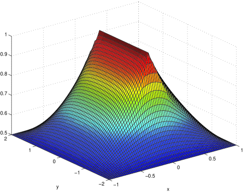
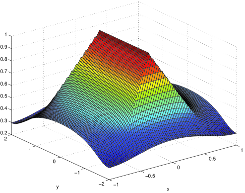
A variant of the above problem is also considered. In this case we assume homogeneous Neumann boundary conditions and a non vanishing forcing function $f$ constantly equal to $-1$. The Neumann boundary conditions have been discretized by using the standard 3-points second order forward an backward difference scheme. After eliminating the boundary unknowns, the associated PLS has always dimension $n=N^{2}$ but in this case the corresponding matrix $T$ satisfies T2 and ${\bf v}={\bf w}$ with all unit components. The forcing term $f$ is such that the right–hand side vector $\bm{b}$ in (8) has negative sum and, thus, Theorem 12 allows us to state that the discrete problem admits a unique solution. Figure 2 shows the plot of the computed numerical solution, whereas in Table 2 we list the number of iterations of (13), $K_{V}$, required to get convergence, for various values of $N$.

Figure 3: Solution of problem (27) with Dirichlet boundary conditions (28), $C=-20$.

Figure 4: Coincidence set (dotted region) related to problem (27) with Dirichlet boundary conditions (28). On the left for $C=-5$ and on the right for $C=-20.$

Figure 5: Coincidence set (dotted region) related to problem (27) with Neumann boundary conditions (30). On the left for $C=-5$ and on the right for $C=-20.$

The second test problem is the elastic-plastic torsion problem in [17],

$$\begin{array}[]{ll}&-\triangle u\geq C,\qquad u(x,y)\geq-\min(x,1-x,y,1-y)\equiv\psi(x,y),\cr&(\Delta u+C)(u-\psi)=0,\qquad(x,y)\in\Omega=(0,1)^{2},\cr\end{array}$$ (27)

where $C<0$ is a given constant, and with homogeneous Dirichlet boundary conditions,

$$u\mid_{\partial\Omega}\equiv\psi\mid_{\partial\Omega}\equiv 0.$$ (28)

It is known that the larger $|C|$, the more difficult the problem. Also in this case, a standard discretization, on a cartesian grid with stepsizes

$$\Delta x=\Delta y=\frac{1}{N+1},$$ (29)

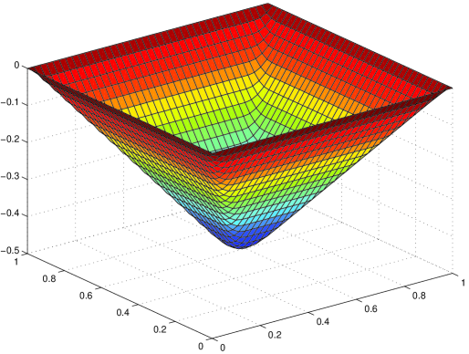
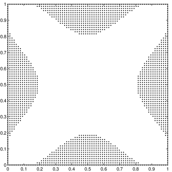
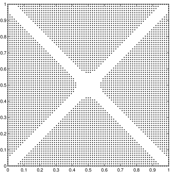
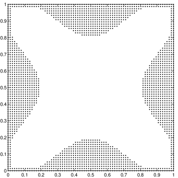
leads to a PLS of dimension $n=N^{2}$, whose matrix $T$ satisfies T1. Figure 3 shows the plot of the computed numerical solution ($C=-20$), whereas in Table 2 we list the number of iterations, $K(C)$, required to get convergence for different values of $C$ and of the discretization parameter $N$ in (29). In such a case, the number of the required iterations of (24) decreases, as $|C|$ increases. This behaviour can be explained considering that, as $|C|$ increases, the coincidence set, i.e. the set of points in $\Omega$ where $u=\psi,$ enlarges, as shown in Figure 5. Consequently, our initialization becomes nearer to the solution. In fact, in our iterative procedure (13) we assume $P^{0}=O;$ thus $\bm{x}^{1}=\bm{b}$ and, for sufficiently fine grids, the negativity of $C$ and the analytical expression of the obstacle function imply that all, or almost all, the components of $\bm{b}$ are negative. Thus, as the solution $\bm{u}$ of (5) is initialized with $\max\{{\bf 0},\bm{x}^{1}\}+\bm{\psi},$ its initialization in this case is almost everywhere coincident with the obstacle and, thus, closer and closer to the final solution as $|C|$ is increased.

Table 1: Numerical results for problem (25) and its Neumann variant, both discretized with stepsizes (26); $K$ and $K_{V}$ respectively denote the number of iterations of (13) for problem (25) and for its variant.

$N$ 25 50 75 100 $n$ 625 2500 5625 10000 $K$ 6 10 10 12 $K_{V}$ 12 25 37 49

Table 2: Numerical results for problem (27) discretized with stepsizes (29), either with Dirichlet boundary conditions (28) or with Neumann boundary conditions (30); $K(C)$ denotes the number of iterations of (13) for the specified value of the parameter $C$.

$N$ 25 50 75 100 $n$ 625 2500 5625 10000 $K(C=-5)$ 9 17 25 32 $K(C=-10)$ 5 10 13 16 $K(C=-15)$ 4 7 9 11 $K(C=-20)$ 4 5 7 9

Even for this problem we have considered a variant with Neumann boundary conditions, which have been chosen in order to get a solution with a shape analogous to that of the solution of the Dirichlet problem. In more detail, (28) is replaced by the following non homogeneous Neumann boundary conditions,

$$\left.\frac{\partial u}{\partial n}\right|_{\partial\Omega}=\left.\frac{\partial\psi}{\partial n}\right|_{\partial\Omega},$$ (30)

where a suitable extension of the derivative of $\psi$ at the corner points of the domain is used. By using again a second order discretization of the boundary conditions and eliminating the boundary unknowns, the problem dimension is unchanged and, as for the variant of the first problem, we deal with a matrix $T$ satisfying T2, and ${\bf v}={\bf w}$ with all unit components. Also in this case, from Theorem 12, we obtain a unique solution for the associated discrete problem. For all the values of $N$ and $C$ considered in Table 2, as outlined in the caption of the table, convergence has been obtained with the same number of iterations as for the Dirichlet case. No plot of the solution is reported for this problem with Neumann conditions because, for all the considered values of $C,$ it is analogous to that related to the Dirichlet case. We only present the obtained coincidence sets in Figure 5 which, when compared with the corresponding ones in Figure 5, better show the small difference near the boundary between the obtained solution and that related to the Dirichlet case.

6.2 The parabolic obstacle problem

The problems that we shall consider here, are evolutionary versions of those considered in Section 6.1. In more details, the first problem is given by

$$u_{t}\geq\triangle u,\qquad u(x,y,t)\geq\psi(x,y),\qquad(u_{t}-\Delta u)(u-\psi)=0,$$

(31)

$$(x,y,t)\in\Omega\times(0,\tau],\qquad u\mid_{\partial\Omega}\equiv\frac{1}{2},\qquad u\mid_{t=0}=\max\left(\psi,\frac{1}{2}\right),$$

where $\psi$ and $\Omega$ are the same items defined in (25). The spatial discretization is the same used for that problem (see (26)), whereas the discretization in time is, for sake of simplicity, done by means of the implicit Euler method, by using a constant stepsize

$$\Delta t=\frac{\tau}{\nu},$$ (32)

being $\nu$ the number of time steps. The resulting PLS, to be solved at each time step, has dimension $n=N^{2}$, whose matrix $T$ is the same as that obtained for problem (25). Table 3 summarizes the obtained results, in terms of required number of iterations, for $\tau=10^{4}$ and $\nu=20$. In such a case, the approximation at $t=\tau$ is quite close to the limit solution plotted in Figure 2. Here the number of iterations of (24) appears to be independednt of spatial resolution.

Table 3: Number of iterations for problem (31), discretized with stepsizes (26) and (32), at each timestep $i\Delta t$, $i=1,\dots,20$.

$N$ 25 50 75 100 $i\backslash n$ 625 2500 5625 10000 $1$ 5 6 8 8 $2$ 5 6 6 6 ⋮ ⋮ ⋮ ⋮ ⋮ $20$ 5 6 6 6

The second test problem is the evolutionary version of the elastic-plastic torsion problem (27):

$$u_{t}\geq\Delta u+C,\quad u(x,y,t)\geq\psi(x,y),\quad(u_{t}-\Delta u-C)(u-\psi)=0,$$

(33)

$$(x,y,t)\in\Omega\times(0,\tau],\qquad u\mid_{\partial\Omega}\equiv 0,\qquad u\mid_{t=0}=\max\left(\psi,0\right)\equiv 0,$$

where $\psi$ and $\Omega$ are the same items defined in (27). The spatial discretization is the same used for that problem (see (29)), whereas the discretization in time is, for sake of simplicity, done by means of the implicit Euler method, by using a constant stepsize (32). Also in this case, the resulting PLS, to be solved at each time step, has dimension $n=N^{2}$, whose matrix $T$ is the same as that obtained for problem (27). Table 4 summarizes the obtained results, in terms of required number of iterations, for $\tau=5$ and $\nu=20$. In such a case, the approximation at $t=\tau$ is quite close to the limit solution plotted in Figure 3. The number of iterations required for obtaining the solution turns out to be quite similar to that listed in Table 2 for the corresponding stationary problem.

Table 4: Number of iterations for problem (33), discretized with stepsizes (29) and (32), at each timestep $i\Delta t$, $i=1,\dots,20$.

$N$ 25 50 75 100 $n$ 625 2500 5625 10000 $i\backslash C$ -5 -10 -15 -20 -5 -10 -15 -20 -5 -10 -15 -20 -5 -10 -15 -20 $1$ 9 5 4 4 17 10 7 5 25 13 9 7 32 16 11 9 $\vdots$ $\vdots$ $\vdots$ $\vdots$ $\vdots$ $\vdots$ $\vdots$ $\vdots$ $\vdots$ $\vdots$ $\vdots$ $\vdots$ $\vdots$ $\vdots$ $\vdots$ $\vdots$ $\vdots$ $20$ 9 5 4 4 17 10 7 5 25 13 9 7 32 16 11 9

7 Conclusions

Two simple semi-iterative Newton-type procedures for solving certain classes of piecewise linear systems have been investigated. Such piecewise linear systems are derived from the efficient modeling of obstacle problems. It has been shown that, under rather general assumptions, the iterates are well defined and monotonically converge to an exact solution of the given system in a finite number of steps. A few numerical examples, concerning both the classical obstacle problem, and its evolutionary (i.e., parabolic) counterpart, prove the effectiveness of the proposed methods.

Acknowledgements

The authors are indebted with Prof. V. Casulli for his valuable comments.

References

- [1] Y. Achdou, F. Hecht, D. Pommier. A Posteriori Error Estimates for Parabolic Variational Inequalities. J. Sci. Comput. 37 (2008) 336–366.
- [2] L. Brugnano, V. Casulli. Iterative solution of piecewise linear systems, SIAM Journal on Scientific Computing 30 (2008) 463–472.
- [3] L. Brugnano, V. Casulli. Iterative solution of piecewise linear systems and applications to flows in porous media, SIAM Journal on Scientific Computing 31 (2009) 1858–1873.
- [4] G. Fichera. Problemi elastostatici con vincoli unilaterali: il problema di Signorini con ambigue condizioni al contorno. Atti Accad. Naz. Lincei Mem. Cl. Sci. Fis. Mat. Nat. Sez. Ia 7(8) (1963-1964) 91–140.
- [5] R. Glowinski. Numerical Methods for Nonlinear Variational Problems. Springer Verlag, New York, NY, 1984.
- [6] W. Hackbusch, H. Mittelmann. Multigrid Methods for Variational Inequalities. Numer. Math. 42 (1983) 65–76.
- [7] R. Hoppe, Multigrid Algorithms for Variational Inequalities. SIAM J. on Numer. Anal. 24 (1987) 1046–1065.
- [8] R.H.W. Hoppe, R. Kornhuber. Adaptive multilevel methods for obstacle problems. SINUM 31 (1994) 301–323.
- [9] K. Ito, K. Kunisch. Parabolic Variational Inequalities: the Lagrange Multiplier Approach. J. Math. Pures Appl. 85 (2006) 415–449.
- [10] C. Kanzow. Inexact semismooth Newton methods for large-scale complementary problems, Optimization Methods and Software 19 (2004) 309–325.
- [11] T. Kärkkäinen, K. Kulisch, P. Tarvainen. Augmented Lagrangian Active Set Methods for Obstacle Problems. J. of Opt. Theory and Appl. 119 (2003) 499–533.
- [12] J.L. Li, H.P. Ma. Residual-type a posteriori error estimate for parabolic obstacle problems. J. of Shanghai Univerisity (English Edition) 10 (2006) 473–478.
- [13] J.L. Lions, G. Stampacchia. Variational Inequalities. Comm. Pure Appl. Math. 20 (1967) 493–519.
- [14] A. Petrosyan, H. Shahgholian. Parabolic obstacle problems applied to finance. in Recent developments in nonlinear PDEs, 117–133, Contemp. Math. 439 AMS, 2007.
- [15] J.-F. Rodrigues. Obstacle Problems in Mathematical Physics. North-Holland, 1987.
- [16] Y. Saad. Iterative Methods for Sparse Linear Systems, 2nd Edition, SIAM, Philadelphia, PA, 2003.
- [17] L. Xue, X.-L. Cheng. An algorithm for solving the obstacle problems. Computers Math. Appl. 48 (2004) 1651–1657.
- [18] Y. Zhang. Multilevel projection algorithm for solving obstacle problems. Computers Math. Appl. 41 (2001) 1505–1513.