Multi-Way, Multi-View Learning

Abstract

We extend multi-way, multivariate ANOVA-type analysis to cases where one covariate is the view, with features of each view coming from different, high-dimensional domains. The different views are assumed to be connected by having paired samples; this is a common setup in recent bioinformatics experiments, of which we analyze metabolite profiles in different conditions (disease vs. control and treatment vs. untreated) in different tissues (views). We introduce a multi-way latent variable model for this new task, by extending the generative model of Bayesian canonical correlation analysis (CCA) both to take multi-way covariate information into account as population priors, and by reducing the dimensionality by an integrated factor analysis that assumes the metabolites to come in correlated groups.

1 Introduction

Finding disease and treatment effects from populations of measurements is a prototypical multi-way modeling task, traditionally solved with multivariate ANOVA. Here disease state (diseased/healthy) and treatment (treated/placebo) are the two covariates, and the research question is, are there differences in the population that can be explained by either covariate or, more interestingly, their interaction, which would hint at the treatment being effective. It is naturally additionally interesting what the differences are.

A recurring problem in multi-way analyses, especially with modern high-throughput measurements in molecular biology, is the ”small $n$, large $p$”-problem. The dimensionality $p$ of the measurements is high while the number of samples $n$ is low, and additionally the data may be collinear making estimation of the effects impossible with classical methods, univariate or multivariate linear models solved with multi-way ANOVA techniques. The most promising modern method, Bayesian sparse factor regression model [1], is useful in finding the variables most strongly related to the external covariate and to infer relationships between those variables via common latent factors. Instead of a regression model we will use a generative latent factor model which incorporates an assumption of clusteredness of the variables to regularize the model, and makes it possible to extend the model to multi-view factor analysis. Such clusteredness is well justified in our application field, metabolomics, where due to biochemical reaction pathways the variation in concentrations of metabolite groups is highly correlated [2].

Assume that measurements have been made on the same objects but with different methods, resulting in different data sources possibly on different domains. An example we will analyze in this paper is metabolomic profiles in different tissues, where the domains are partly different since the metabolites cannot be fully matched. The different views form one covariate in the multi-way analysis, with the additional problem that the samples come from different domains and cannot be directly compared. We introduce a new hierarchy level of latent variables intended to decompose the views into view-specific and shared components, which is needed for the multi-way analysis. Such a decomposition is possible given that the samples in the different views come in pairs, which we need to assume.

The resulting decomposition between the views turns out to be implementable with Bayesian canonical correlation analysis [3, 4, 5], interpretable as unsupervised multi-view modeling. Hence, in this work we re-interpret unsupervised multi-view modeling as one-way modeling of samples from different domains, and combine it with multi-way modeling. Given that we additionally can work under the large p, small n conditions, the model is expected to have widespread applicability in current molecular biological measurements.

2 Model

2.1 Multi-way, multi-view

We will generalize ANOVA to multi-view (multi-domain) analysis, restricting to two covariates and two views for simplicity. Using ANOVA-style notation and assuming the views to be in the same domain, the multivariate linear model for samples is

$${\bf v}_{d}=\boldsymbol{\alpha}_{a}+\boldsymbol{\beta}_{b}+(\boldsymbol{\alpha\beta})_{ab}+\boldsymbol{\gamma}_{d}+(\boldsymbol{\alpha\gamma})_{ad}+(\boldsymbol{\beta\gamma})_{bd}+(\boldsymbol{\alpha\beta\gamma})_{abd}+\text{noise},$$ (1)

where $a$ and $b$ ($a=0,\dots A$ and $b=0,\dots B$), are the two traditional independent covariates such as disease and treatment, and $d$ denotes the view.

For different values of $d$ the domain of ${\bf v}^{d}$ may vary, meaning different feature spaces with different dimensionalities. We assume the samples of the different views to come in pairs, $\mathbf{v}=[\mathbf{x},\mathbf{y}]$. For the rest of the paper we will change the notation for clarity to $\mathbf{v}^{1}=\mathbf{x}$, $\mathbf{v}^{2}=\mathbf{y}$, and assume a mapping $f^{x}$ from the effects to the domain of $\mathbf{x}$ which is linear for now. Then,

$${\bf x}=f^{x}(\boldsymbol{\alpha}_{a}+\boldsymbol{\beta}_{b}+(\boldsymbol{\alpha\beta})_{ab})+f^{x}((\boldsymbol{\alpha})^{x}_{a}+(\boldsymbol{\beta})^{x}_{b}+(\boldsymbol{\alpha\beta})^{x}_{ab})+\text{noise},$$ (2)

assuming $\gamma_{d}=0$, because it does not make sense to compare means of different domains, and that the view-specific effects are in the same domain as the view-independent effects and hence need to be transformed with the same function. The equation for $\mathbf{y}$ is analogous.

To our knowledge, there exists no method capable of studying the view-independent, and view-dependent effects. In the next section we will introduce a model which will additionally assume that the effects may be uncertain, resulting in a hierarchical Bayesian model.

2.2 Hierarchical model

We next formulate a hierarchical latent-variable model for the task of multi-way, multi-view learning under “large $p$, small $n$” conditions. For this we need three components: (i) regularized dimension reduction, (ii) combination of different data domains, and (iii) multi-way analysis. We formulate each of these as part of a big generative model. We will first summarize the main components of the model shown in Figure 1, and then describe each part in detail.

Figure 1: The hierarchical latent-variable model for multi-way, multi-view learning under “large $p$, small $n$” conditions.

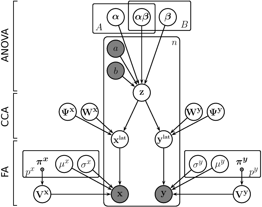
To deal with the small sample size $n\ll p$ problem, we reduce the dimensionality of the data $\mathbf{x}$ and $\mathbf{y}$ from the two views into their respective latent variables $\mathbf{x}^{lat}$ and $\mathbf{y}^{lat}$. This is done with factor analyzers which assume that the variables come in groups, which is a strongly regularizing assumption effective under the “large $p$, small $n$” conditions. The clustering assumption is particularly sensible under the assumption that metabolomics data, our main application, contains strongly correlated groups of variables [2].

The second necessary element is search for a view shared by the two different domains $\mathbf{x}$ and $\mathbf{y}$, needed for finding shared multi-way effects. Given paired data, this is a task for Bayesian CCA (BCCA) [3, 4, 5] which introduces a new hiearchy level where a latent variable $\mathbf{z}$ captures the shared variation between the views. The view-specific variation has been implicitly modeled by view-specific latent variables which have been integrated out, resulting in flexible covariance matrices parameterized by the $\boldsymbol{\Psi}$.

The third necessary element, the ANOVA-type two-way analysis is supplemented by assigning the effect terms as priors on the latent variables $\mathbf{z}$; in normal BCCA the prior is zero-mean. The observed covariates $a$ and $b$ choose the correct effects for each sample. The covariates hence effectively change the means of the data as in eqn (2), and the variation around the mean is modeled with the rest of the model. The central differences from (2) are that the model is hierarchical, implying that the arguments of the linear function $f^{x}$ have a distribution, and that the “noise” is structured, stemming from all the latent variables. With these additions, the model will be better able to take into account the uncertainty in the data.

The posterior is computed with Gibbs sampling. The Gibbs-formulas are included in the supplementary material.

In effect the model, shown in Figure 1, consists of two factor analyzers, where the loadings assume cluster memberships (multiplied with scales), a generative model of CCA, and population-specific priors on $\mathbf{z}$ that assume ANOVA-type multi-way structure. We will now introduce the details of each of these parts in turn.

2.2.1 Factor analysis model

We need to reduce dimensionality, which can be done by factor analysis (FA). The model [6] for $n$ exchangeable replicates is

$$\mathbf{x}_{j}^{lat}\sim\mathcal{N}(0,\boldsymbol{\Psi}^{x})$$

$$\mathbf{x}_{j}\sim\mathcal{N}({\boldsymbol{\mu}^{x}}+\mathbf{V}^{x}\mathbf{x}_{j}^{lat},\boldsymbol{\Lambda}^{x})\;.$$ (3)

Here $\boldsymbol{V}^{x}$ is the projection matrix that is assumed to generate the data vector $\mathbf{x}_{j}$ from the latent variable $\mathbf{x}_{j}^{lat}$. The $\mathbf{x}_{j}^{lat}$ is a latent variable vector, whose elements are known as factor scores. The $\mathbf{V}^{x}\mathbf{x}^{lat}_{j}$ models such common variance of the data around the variable-means ${\boldsymbol{\mu}^{x}}$ that can be explained by factors common to all or many variables, effectively estimated from the sample covariance matrix of the dataset. The sample covariance becomes decomposed into $\hat{\boldsymbol{\Sigma}}=\mathbf{V}^{x}\mathbf{V}^{xT}+\boldsymbol{\Lambda}^{x}$, where ${\boldsymbol{\Lambda}^{x}}$ is a diagonal residual variance matrix with diagonal elements $\sigma_{i}^{2}$, modelling the variable-specific noise not explained by the latent factors. The covariance matrix of $\mathbf{x}^{lat}$, $\boldsymbol{\Psi}^{x}$, comes from the CCA.

At this point, when $n<p$, $\mathbf{V}^{x}$ cannot be estimated due to the singularity of the sample covariance matrix. To overcome the $n\ll p$ problem, we now restrict $\mathbf{V}^{x}$ to a non-singular clustering matrix, suitable for data containing highly correlated groups of variables.

2.2.2 Projection matrix that assumes grouped variables

We make the structured assumption that there are strongly correlated groups of variables in the data, the generated values within the whole group being governed by one latent variable. The projection matrix $\mathbf{V}^{x}$ is positive-valued, each row having one non-zero element corresponding to the cluster assignment of the variable,

$$\mathbf{V}^{x}=\left[\begin{array}[]{ccc}\lambda_{1}&0&0\\ 0&0&\lambda_{2}\\ \vdots&\vdots&\vdots\\ 0&\lambda_{j}&0\\ 0&\lambda_{j+1}&0\\ \vdots&\vdots&\vdots\\ \end{array}\right]\;.$$ (4)

The location of the non-zero value on row $i$, $v_{i}$, follows a multinomial distribution with one observation, with an uninformative prior distribution $\boldsymbol{\pi}_{i}$. The $\boldsymbol{\pi}_{i}$ could also be used to encode prior information on the known grouping of variables. The variation of each variable within a cluster is assumed to be modeled by the same latent variable, but the scales $\lambda_{i}$ may differ. The variable-specific residual variances $\sigma_{i}^{2}$, that are the diagonal elements of $\boldsymbol{\Lambda}$, follow a scaled $\textrm{Inv-}\chi^{2}$ with an uninformative prior.

In summary, we regularize the covariance matrix by assuming that the main correlations are positive correlations between variables belonging to the same cluster. This correlation is mediated through a common latent variable; this is a reasonable assumption for metabolomics data and, furthermore, facilitates interpretation of the results.

2.2.3 Generative model of CCA

We need to combine different data domains, and for paired data that can be done with CCA. The generative model of BCCA has been formulated [3, 7] for sample $j$ as

$$\mathbf{z}_{j} \sim N(0,\mathbf{I}),$$

$$\mathbf{x}^{lat}_{j} \sim N(\mathbf{W}^{x}\mathbf{z}_{j},\mathbf{\Psi}^{x}),$$ (5)

and likewise for $\mathbf{y}$. Here we have assumed no mean parameter since the mean of the data is estimated in the factor analysis part. The $\mathbf{W}^{x}$ is a projection matrix from the latent variables $\mathbf{z}_{j}$, and $\mathbf{\Psi}^{x}$ is a matrix of marginal variances. The crucial thing is that the latent variables $\mathbf{z}$ are shared between the two data sets, while everything else is independent. The prior distributions were chosen as

$$\mathbf{w}_{l} \sim N(0,\beta_{l}\mathbf{I}),$$

$$\beta_{l} \sim IG(\alpha_{0},\beta_{0}),$$

$$\mathbf{\Psi}^{x},\mathbf{\Psi}^{y} \sim IW(\mathbf{S}_{0},\nu_{0}).$$ (6)

Here $\mathbf{w}_{l}$ denotes the $l$th column of $\mathbf{W}$, and $IG$ and $IW$ are shorthand notations for the inverse Gamma and inverse Wishart distributions. The priors for the covariance matrices $\mathbf{\Psi}^{x}$ and $\mathbf{\Psi}^{y}$ are conventional conjugate priors, and the prior for the projection matrices is the so-called Automatic Relevance Determination (ARD) prior used for example in Bayesian principal component analysis [8].

2.2.4 ANOVA-type model for latent variables.

We assume that the ANOVA-type effects act on the latent variables $\mathbf{z}$, which allows access to effects found in both the spaces $\mathbf{x}^{lat}$ and $\mathbf{y}^{lat}$. They are modeled as population priors to the latent variables, which in turn are given Gaussian priors $\boldsymbol{\alpha}_{a}$, $\boldsymbol{\beta}_{b}$, $(\boldsymbol{\alpha\beta})_{ab}\sim\mathcal{N}(0,\mathbf{I})$.

In the $K_{z}$-dimensional latent variable space we then have

$$\mathbf{z}_{j}=\boldsymbol{\alpha}_{a}+\boldsymbol{\beta}_{b}+(\boldsymbol{\alpha\beta})_{ab}+\boldsymbol{\epsilon}_{j},$$ (7)

where $\boldsymbol{\epsilon}_{j}$ is a noise term. Note that the grand means are estimated in the lower level of hierarchy, that is, directly in the $\mathbf{x}$ and $\mathbf{y}$-spaces, and do not appear here.

To simplify the interpretation of the effects we center the grand means to the mean of one control population. A similar choice has been done successfully in other ANOVA studies [9], and it does not significantly sacrifice generality. We set the parameter vector $\boldsymbol{\mu}^{x}$, describing variable-specific means, to the mean of the control group. One group now becomes the baseline to which other classes are compared by adding main and interaction effects. For convenience, we will additionally change the variables compared to the standard ANOVA convention, such that the terms $\boldsymbol{\alpha}_{0}$, $\boldsymbol{\beta}_{0}$, $\boldsymbol{\alpha\beta}_{00}$, $(\boldsymbol{\alpha\beta})_{0b}$, and $(\boldsymbol{\alpha\beta})_{a0}$ are not estimated. The differences between the populations are now modelled directly with $\mathbf{x}^{lat}$ and $\mathbf{y}^{lat}$, and hierarchically by the main effects $\boldsymbol{\alpha}_{a}$, $\boldsymbol{\beta}_{b}$, $(\boldsymbol{\alpha\beta})_{ab}$, $a,b>0$.

In our case study, $a$ and $b$ have only two values and we have populations $(a,b)={(0,0),(1,0),(0,1),(1,1)}$, and there are hence three terms $\boldsymbol{\alpha}_{1}$, $\boldsymbol{\beta}_{1}$ and $(\boldsymbol{\alpha\beta})_{11}$, that model the difference to the control population $(a,b)=(0,0)$.

In summary, the complete hierarchical model of Figure 1 is

$$\boldsymbol{\alpha}_{0}=0,\boldsymbol{\beta}_{0}=0,(\boldsymbol{\alpha\beta})_{a0}=0,(\boldsymbol{\alpha\beta})_{0b}=0$$

$$\boldsymbol{\alpha}_{a},\boldsymbol{\beta}_{b},(\boldsymbol{\alpha\beta})_{ab}\sim\mathcal{N}(0,\mathbf{I})$$

$${\mathbf{z}}_{j}|_{j\in a,b}\sim N(\boldsymbol{\alpha}_{a}+\boldsymbol{\beta}_{b}+(\boldsymbol{\alpha\beta})_{ab},\mathbf{I})$$

$${\mathbf{x}}_{j}^{lat}\sim N(\mathbf{W}^{x}\mathbf{z}_{j},\boldsymbol{\Psi}^{x})$$

$${\mathbf{x}}_{j}\sim\mathcal{N}({\boldsymbol{\mu}}^{x}+{\mathbf{V}}\mathbf{x}_{j}^{lat},{\boldsymbol{\Lambda}^{x}}).$$ (8)

2.3 Decomposing covariate effects into shared and view-specific

Figure 2: The graphical model describing the decomposition of covariate effects into shared and view-specific ones. The figure expands the top part of Figure 1, leaving out the feature extraction part and some parameters.

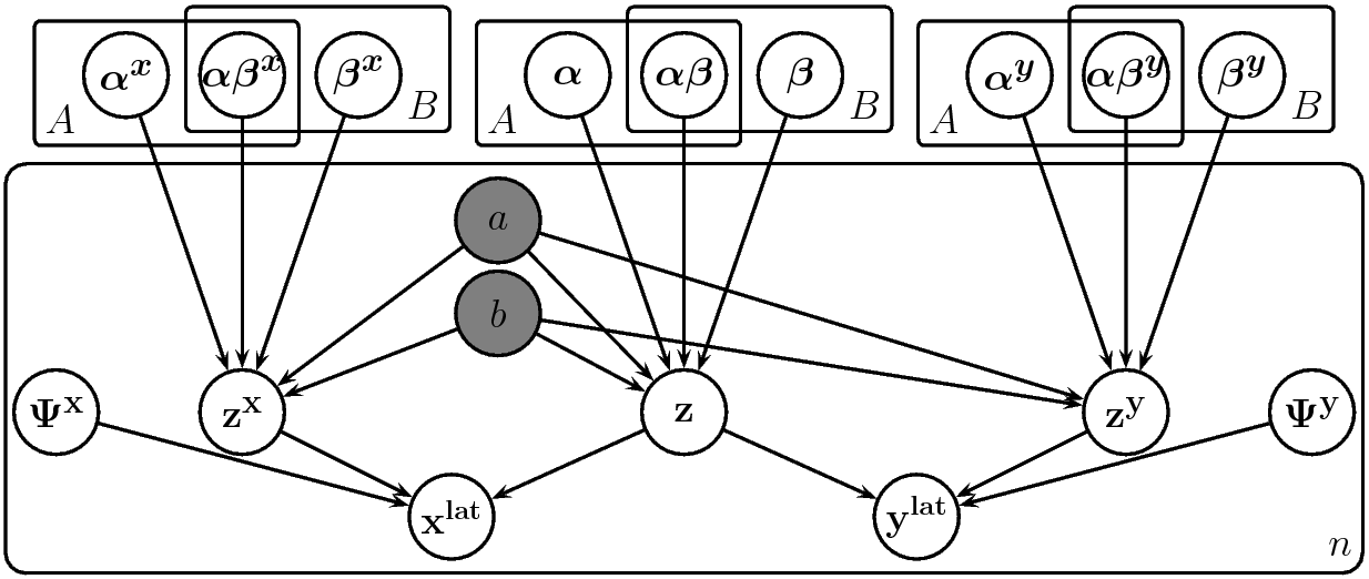
So far we have not discussed how the model finds the view-related effects or, in our application, tissue effects $\boldsymbol{\alpha}_{a}^{x}$, $\boldsymbol{\beta}_{b}^{x}$, and $(\boldsymbol{\alpha\beta})_{ab}^{x}$, and likewise for $y$.

The Bayesian CCA assumes that the data is generated by a sum of view-specific latent variables $\mathbf{z}^{x}$ and $\mathbf{z}^{y}$, and shared latent variables $\mathbf{z}$, and the former have been integrated out in the graphical model of Figure 1. The way to implement the view-specific effects is to assign them as priors to the view-specific latent variables. Then we do not want to integrate them out but include them explicitly in the model as shown in Figure 2.

As a technical note, to make computation of the model faster and more reliable, we have further included view-specific latent variables that do not have disease or treatment effects. They have been integrated out, resulting in the covariance parameters $\boldsymbol{\Psi}$ in Figure 2. Their role is to explain away all or most of the variation that is unrelated to the disease and treatment effects, so that Gibbs sampling does not need to model all that variation. This trick should not change modeling results in the limit of an infinite time for computation.

In practice the decomposition in Figure 2 is implemented by restricting a column of $\mathbf{W}^{x}$ to be zero for the y-specific components and vice versa for x.

2.4 Data preprocessing and model complexity selection

For simplicity and to reduce the number of parameters of the model, the data is preprocessed such that for each variable the mean of the control population $a=0$, $b=0$ is subtracted and the variable is scaled by the standard deviation of the control population. This fixes the scales $\lambda_{i}$ to one and the $\boldsymbol{\mu}^{x}$ and $\boldsymbol{\mu}^{y}$ to zero. The factor analysis part now models correlations of the variables. The possible covariate effects are now comparable to the control population as discussed in Chapter 2.2.4

Model complexity, that is, the number of clusters and latent variables, is chosen separately for both $\mathbf{x}^{lat}$ and $\mathbf{y}^{lat}$ by predictive likelihood in 10-fold cross-validation.

3 Results

We demonstrate the working of the method on generated data, and apply it to a disease study where lipidomic profiles have been measured from several tissues of model mouse samples, under a two-way experimental setup (disease and treatment), the two feature spaces (lipid profiles) are distinct and samples paired.

3.1 Generated data

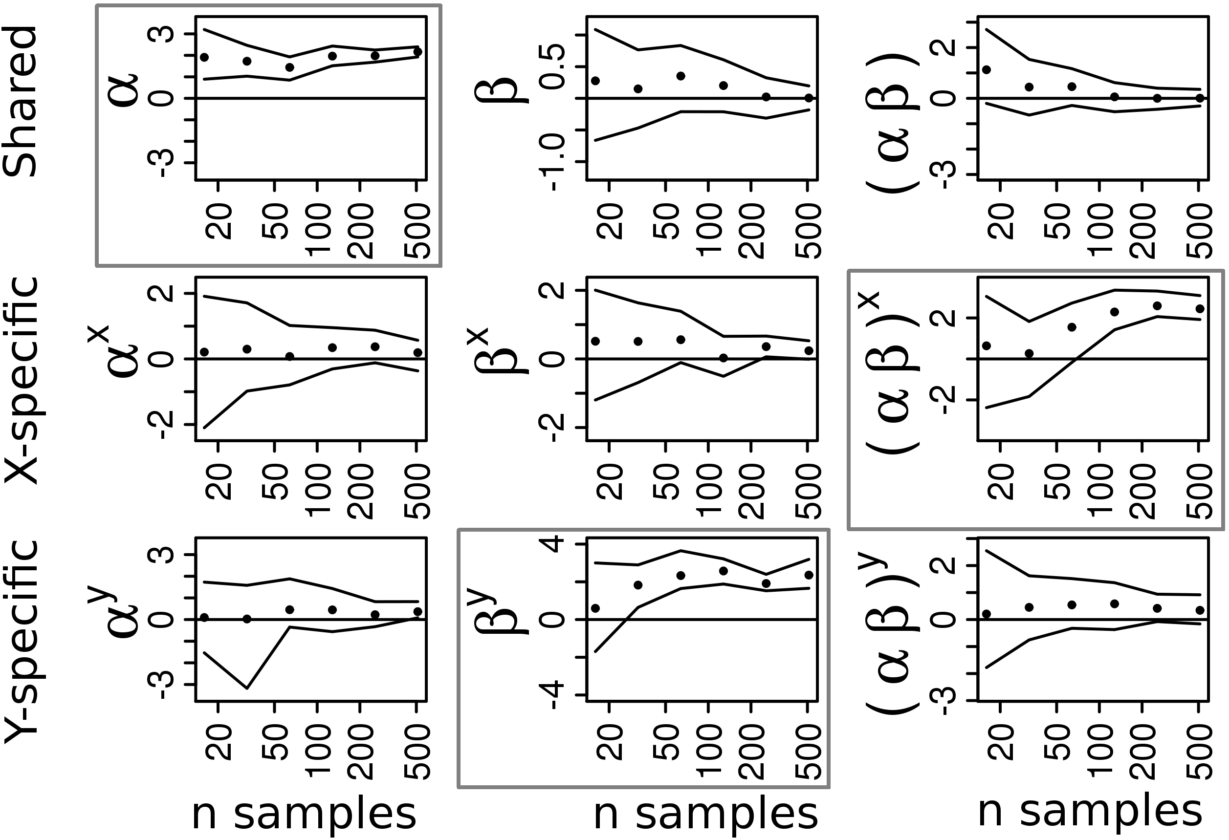
We generate data having known effects, and then study how well the model finds the effects as a function of the number of measurements. There are three effects, in $\alpha$, $\beta^{y}$, and $(\alpha\beta)^{x}$.

Each of the three effects have strength $+2$, the $\mathbf{x}^{lat}$ and $\mathbf{y}^{lat}$ are both 3-dimensional, and the $\mathbf{x}$ and $\mathbf{y}$ are 200-dimensional. The $\sigma_{i}=1$ for each variable $i$ in $\mathbf{x}$ and $\mathbf{y}$. The model is computed by Gibbs sampling, discarding 1000 burn-in samples, and collecting 1000 samples for inference. To fix the sign of the effects without affecting the results, each posterior distribution is mirrored, if necessary, to have a positive mean, i.e. multiplied by the sign of the posterior mean.

The method finds the three generated effects, shown in Figure 3. The uncertainty decreases with increasing number of observations. The shared effect is found with much less uncertainty since there is evidence from both views. With low numbers of samples, there is considerable uncertainty in the effects for view-specific components. In typical bioinformatics applications there may be 20-50 samples.

Figure 3: The method finds the generated effects $\alpha=+2$,$\beta^{y}=+2$, and $(\alpha\beta)^{x}=+2$. (effect subscripts ₁ and ₁₁ have been dropped in the rest of the results section). The dots show posterior mean and the thin lines include 95% of posterior mass, as a function of number of observations. A consistently non-zero posterior distribution implies an effect found.

3.2 Lung cancer study

We then study data from a two-way, two-view, $n\ll p$, so far unpublished lung cancer mouse model experiment. The diseased mice are compared to healthy control samples and, in addition, some mice from both groups have been given a test anticancer drug treatment. There are thus healthy untreated (9 mice/samples), diseased untreated (7), healthy treated (6) and diseased treated (6) samples. Lipidomic profiles have been measured by Liquid Chromatography Mass Spectrometry. The study has a two-way experimental setup, such that disease effect $\alpha$, treatment effect $\beta$ and an interaction effect $\alpha\beta$ on lipid groups are to be estimated. The high-dimensional lipidomic profiles have been measured from several tissues of each mouse; the tissues have partly different lipids that have not been matched, and even the roles of the matched lipids may be different in different tissues. Hence, the tissues have different feature spaces with paired samples, implying a two-view study. We will specifically study the relationship between blood and lung tissue, which is the most interesting for diagnosis, since blood can be easily sampled.

3.2.1 Experiment 1. Effects shared by blood and disease tissue

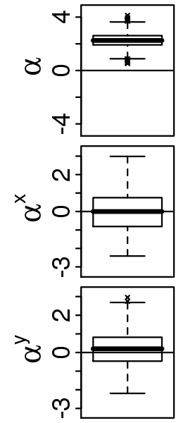
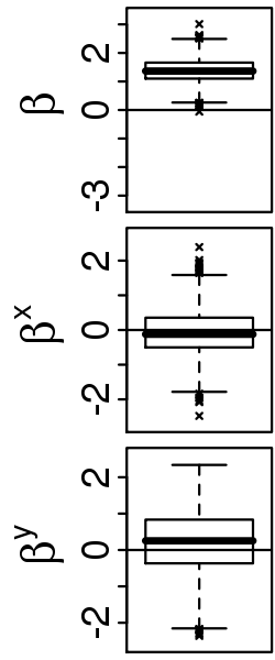
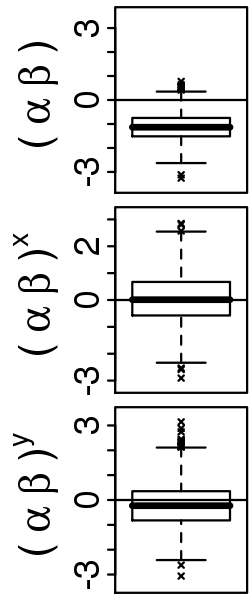
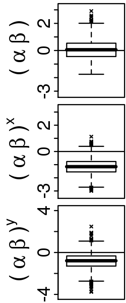
Blood plasma (168 lipids) and lung tissue (68 lipids) were integrated with the method. The optimal number of clusters for plasma was 6 and for lung 5, found by predictive likelihood. The method finds a disease effect $\alpha$ and treatment effect $\beta$ shared by both views (Fig. 4). The effect can be traced back to the metabolite groups, by first identifying the responsible row of $\mathbf{W}^{x}$ and hence component of $\mathbf{x}^{lat}$, and then the metabolite cluster from the $\mathbf{V}^{x}$ corresponding to the $\mathbf{x}^{lat}$ component.

The results imply that a cluster of 12 lipids in lung and a cluster of 20 lipids in blood are mutually coherently up-regulated due to disease, and additionally up-regulated by the treatment. Another cluster of 13 lipids in lung was found down-regulated due to the disease and additionally down-regulated due to treatment. The lipids of the down-regulated cluster are thus negatively correlated with the up-regulated clusters. The results show that since no consistent interaction term $(\alpha\beta)$ is found, there is no indication that the treatment would cure the cancer effects. This confirms our prior fear that the specific treatment might not be efficient. The treatment does, however, affect the same groups of lipids as the disease, so investigating it as a potential cure was not a far-fetched hypothesis.

The up-regulated cluster of blood plasma contains abundant triglycerides known to be coregulated, the up-regulated cluster of lung contains lipotoxic ceramides [10] and proinflammatory lysophosphatidylcholines [11], while the down-regulated cluster of lung contains ether lipids, known as endogenous antioxidants [12]. Our analysis reveals that the drug treatment enhances, not diminishes, the proinflammatory lipid profile found in the disease.

Experiment 1			Experiment 2

Figure 4: In experiment 1 (left), the method finds a disease effect $\alpha$ and a treatment effect $\beta$ shared between the two views, plasma ($\mathbf{x}$) and lung ($\mathbf{y}$) tissues. In experiment 2 (right), only view-specific effects are found for plasma ($\mathbf{x}$) when integrating with the heart tissue ($\mathbf{y}$). No effects are found in heart. The boxplots show quartiles and 95% intervals of posterior mass of the effects, a consistently non-zero posterior distribution implies an effect found.

3.2.2 Experiment 2. When connected to non-diseased tissue, only view-specific effects are found

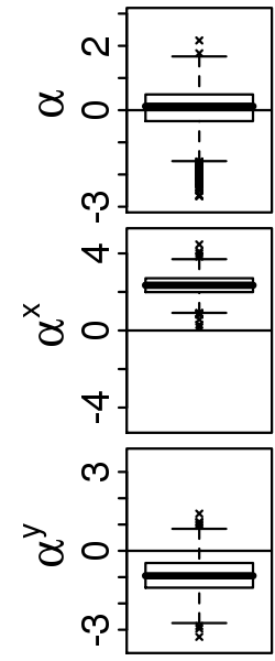
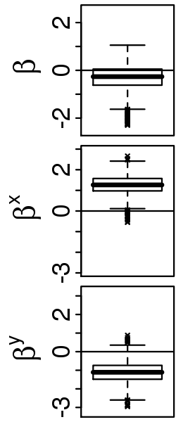
We then integrate plasma $\mathbf{x}$ with another tissue, heart (58 lipids) $\mathbf{y}$. The results ( Figure 4), show that the disease effect and the treatment effect are found only in the view-specific component of plasma. This implies that there are no shared effects between plasma and heart, and in fact no consistent effects are found for the heart tissue. The method finds, however, the same effects, $\alpha$ and $\beta$ in the plasma tissue as in Experiment 1 and for the same cluster of lipids, which is a sign that the method works well.

4 Discussion

We have generalized ANOVA-type multi-way analysis to cases where multiple views of samples having a multi-way experimental setup are available. The problem is solved by a hierarchical latent variable model that extends the generative model of bayesian CCA to model multi-way covariate information of samples by having population-specific priors on the shared latent variable of CCA. Furthermore, the method is able to decompose the covariate effects to shared and view-specific effects, treating the multiple views as one covariate. Finally, the method is designed for cases with high dimensionality and small sample-size, common in bioinformatics applications. The small sample-size problem was solved by assuming that the variables come in correlated groups, which is reasonable for the metabolomics application.

The modelling task is extremely difficult due to the complexity of the task and small sample-size. Hence it was striking that the method was capable of finding covariate effects in a real-world lipidomic multi-view, multi-way dataset.

In this work it was possible to estimate only three components, because the number of samples was extremely low: a shared component and two view-specific components. If more than one shared components are to be estimated, an unidentifiability problem occurs, since there is a rotational ambiguity within the solution subspace. The problem can be solved by a deflation-type method, where the components are computed one by one. Each posterior sample is now considered as a converged starting point, and a second component is added and the model is sampled with having the first component fixed. The last sample of each new sampled chain is collected for inference.

References

- [1] Mike West. Bayesian factor regression models in the large p, small n paradigm. Bayesian Statistics, 7:723–732, 2003.
- [2] Ralf Steuer. Review: On the analysis and interpretation of correlations in metabolomic data. Briefings in Bioinformatics, 7(2):151–158, 2006.
- [3] Arto Klami and Samuel Kaski. Local dependent components. In Zoubin Ghahramani, editor, Proceedings of ICML 2007, the 24th International Conference on Machine Learning, pages 425–432. Omnipress, 2007.
- [4] Chong Wang. Variational Bayesian approach to canonical correlation analysis. IEEE Transactions on Neural Networks, 18:905–910, 2007.
- [5] Cédric Archambeau and Francis Bach. Sparse probabilistic projections. In Daphne Koller, Dale Schuurmans, Yoshua Bengio, and Léon Bottou, editors, Advances in Neural Information Processing Systems 21, pages 73–80. MIT Press, 2009.
- [6] Sam Roweis and Zoubin Ghahramani. A unifying review of linear gaussian models. Neural Computation, 11:305–345, 1999.
- [7] Francis R. Bach and Michael I. Jordan. A probabilistic interpretation of canonical correlation analysis. Technical Report 688, Department of Statistics, University of California, Berkeley, 2005.
- [8] Christopher M. Bishop. Bayesian PCA. In M. S. Kearns, S.A. Solla, and D.A. Cohn, editors, Advances in Neural Information Processing Systems, volume 11, pages 382–388. MIT Press, 1999.
- [9] David M. Seo, Pascal J. Goldschmidt-Clermont, and Mike West. Of mice and men: Sparse statistical modelling in cardiovascular genomics. Annals of Applied Statistics, 1(1):152–178, 2007.
- [10] Scott A. Summers. Ceramides in insulin resistance and lipotoxicity. Progress in Lipid Research, 45:42–72, 2006.
- [11] Dolly Mehta. Lysophosphatidylcholine: an enigmatic lysolipid. American Journal of Physiology Lung Cellular and Molecular Physiology, 289:174–175, 2005.
- [12] Ronald J. A. Wanders Pedro Brites, Hans R. Waterham. Functions and biosynthesis of plasmalogens in health and disease. Biochimica et Biophysica Acta, 1636:219–231, 2004.