Spin and Charge Correlations in Quantum Dots: An Exact Solution Spin and Charge Correlations in Quantum Dots: An Exact Solution

I.S. Burmistrov, Yuval Gefen, and M.N. Kiselev I.S. Burmistrov, Yuval Gefen, and M.N. Kiselev

*

Spin and Charge Correlations in Quantum Dots: An Exact Solution

Abstract

The inclusion of charging and spin-exchange interactions within the Universal Hamiltonian description of quantum dots is challenging as it leads to a non-Abelian action. Here we present an exact analytical solution of the probem, in particular, in the vicinity of the Stoner instabilty point. We calculate several observables, including the tunneling density of states (TDOS) and the spin susceptibility. Near the instability point the TDOS exhibits a non-monotonous behavior as function of the tunneling energy, even at temperatures higher than the exchange energy. Our approach is generalizable to a broad set of observables, including the a.c. susceptibility and the absorption spectrum for anisotropic spin interaction. Our results could be tested in nearly ferromagnetic materials.

73.23.Hk, 75.75.-c, 73.63.Kv

The physics of quantum dots (QDs) is a focal point of research in nanoelectronics. The introduction of the “Universal Hamiltonian” [1, 2] made it possible to simplify in a controlled way the intricate electron-electron interactions within a QD. This provided one with a convenient framework to calculate physical observables. Within this scheme interactions are represented as the sum of three spatially independent terms: charging, spin-exchange, and Cooper channel. Notably, even the inclusion of the first two terms turned out to be non-trivial: the resulting action is non-Abelian  [3, 4]. Attempts to account for those interactions in transport involved a rate equation analysis [5, 6] and a perturbation expansion [4]. Alhassid and Rupp [5] have analyzed some aspects of the problem (see below) exactly. It is known that in the presence of significant spin-exchange interaction such systems can become Stoner unstable. More precisely, one distinguishes 3 regimes of behavior as function of increasing the strength of the exchange interaction: paramagnetic (no zero field magnetization), mesoscopic Stoner regime (finite magnetization whose value increases stepwise with the exchange) and thermodynamic ferromagnetic phase (magnetization is proportional to the volume) [2]. Both the mesoscopic and thermodynamic phases manifest (Stoner) instabilities towards ferromagnetic ordering. The presence of enhanced quantum and statistical fluctuations underlying such instabilities calls for a full-fledged quantum mechanical treatment of the problem.

Here we present an exact analytic algorithm to tackle this challenging problem. We employ our approach to a few physical variables within the mesoscopic Stoner regime, but it can be used to tackle the broad range of problems involving spin and charge on a QD, and be extended to the thermodynamic ferromagnetic regime too. As examples we calculate the following quantities: the partition function, the magnetic susceptibility, the distribution function of the total spin, the tunneling density of states (TDOS), and the sequential tunneling conductance. Our approach allows us to obtain analytic results as one approaches the Stoner instability. Below we list possible applications of our method to other physical observables and extensions beyond the Universal Hamiltonian. The physics discussed here can be best tested in quantum dots with materials which are close to the thermodynamic Stoner instability, e.g., Co impurities in Pd or Pt host, Fe dissolved in various transition metal alloys, Ni impurities in Pd host, and Co in Fe grains, as well as new nearly ferromagnetic rare earth materials  [7, 8].

The main reason why, in this context of a QD, the treatment of the exchange term is non-trivial, is the non-Abelian nature of the action. One needs to tackle time ordered integrals of the form

$$\mathcal{A}_{\gamma}^{(p)}=\mathcal{T}\exp\left(i\int_{0}^{t_{p}}dt^{\prime}\,\bm{\theta}_{p}\bm{s}_{\gamma}\right).$$ (1)

Here $\bm{\theta}_{p}$ is a dynamical, quantum field operating on the spin $\bm{s}_{\gamma}$ (whose $x$ component is proportional to the Pauli matrix $\sigma_{x}$ etc.); $p$ and $\gamma$ are indices to be elaborated below; $\mathcal{T}$ is a time ordering operation. Wei and Norman [9], addressing the problem of a quantum spin subject to a prescribed classical time-dependent magnetic field, have elegantly shown that by preforming a non-linear transformation from $\theta_{p}^{x},\theta_{p}^{y},\theta_{p}^{z}$ to a set of other variables (cf. Eq. (12)), Eq. (1) can be written as a product of 3 Abelian terms (cf. Eq. (13)). Even so, that problem could not be solved. The problem of a quantum field appears to be even more intricate. To solve it we employ here a generalized Wei-Norman-Kolokolov (WNK) method  [10].

We consider a quantum dot of linear size $L$ in the so-called metallic regime, whose dimensionless conductance $g_{\rm Th}=E_{\rm Th}/\delta\gg 1$. Here $E_{\rm Th}$ is the Thouless energy and $\delta$ is the (spinless) mean single particle level spacing. We account for the following terms of the Universal Hamiltonian

$$H=H_{0}+H_{C}+H_{S},\qquad H_{0}=\sum\limits_{\alpha,\sigma}\epsilon_{\alpha}a^{\dagger}_{\alpha,\sigma}a_{\alpha,\sigma}.$$ (2)

Here, $\epsilon_{\alpha}$ denotes the spin ($\sigma$) degenerate single particle levels. The charging interaction $H_{C}=E_{c}\left(\hat{n}-N_{0}\right)^{2}$ accounts for the Coulomb blockade, with $\hat{n}\equiv\sum_{\alpha}\hat{n}_{\alpha}=\sum_{\alpha,\sigma}a^{\dagger}_{\alpha,\sigma}a_{\alpha,\sigma}$ being the particle number operator; $N_{0}$ represents the positive background charge. The term $H_{S}=-J\bm{S}^{2}$ represents spin interactions within the dot ($\bm{S}=\sum_{\alpha}\bm{s}_{\alpha}=\frac{1}{2}\sum_{\alpha}a^{\dagger}_{\alpha,\sigma}\bm{\sigma}_{\sigma\sigma^{\prime}}a_{\alpha,\sigma^{\prime}}$), with the components of $\bm{\sigma}$ comprising of the Pauli matrices.

The imaginary time action for this system reads:

$$S_{\rm tot}=\int_{0}^{\beta}\mathcal{L}d\tau=\int_{0}^{\beta}\Bigl{[}\sum\limits_{\alpha}\bar{\Psi}_{\alpha}(\partial_{\tau}+\mu)\Psi_{\alpha}-H\Bigr{]}d\tau.$$

Here $\mu$ is the chemical potential, $\beta=1/T$, $T$ the temperature, and we have introduced the Grassmann variables $\bar{\Psi}_{\alpha}=(\bar{\psi}_{\alpha\uparrow},\bar{\psi}_{\alpha\downarrow})^{T},\Psi_{\alpha}=(\psi_{\alpha\uparrow},\psi_{\alpha\downarrow})$ to represent electrons on the dot.

Employing a Hubbard-Stratonovich transformation leads to a bosonized form

$$\mathcal{L} = \sum_{\alpha}\bar{\Psi}_{\alpha}\left[\partial_{\tau}-\epsilon_{\alpha}+\mu+i\phi+\frac{\bm{\sigma}\cdot\bm{\Phi}}{2}\right]\Psi_{\alpha}$$

$$+\frac{\bm{\Phi}^{2}}{4J}+\frac{\phi^{2}}{4E_{c}}-iN_{0}\phi$$

where $\phi$ and $\bm{\Phi}$ are scalar and vector bosonic fields respectively. The $SU(2)$ non-Abelian character of the action poses a serious difficulty. It prevents one from performing a gauge transformation [11] which works efficiently in the Abelian $U(1)$ (charging only) case [11, 12, 13]. Employing the Wei-Norman-Kolokolov trick we are able to overcome this difficulty.

Results. — Below we present our main results. The TDOS is given by the following exact expression

$$\nu(\varepsilon)=\frac{1+e^{-\beta\varepsilon}}{Z}\sum_{n_{\uparrow,\downarrow}\in\mathbb{Z}}e^{-\beta E_{c}(n-N_{0})^{2}+\beta\mu n+\beta Jm(m+1)}\hskip 22.76228pt\,{}$$

$$\hskip 14.22636pt\times\sum_{\alpha}\delta\Bigl{[}\varepsilon-\epsilon_{\alpha}+\mu-E_{c}(2n-2N_{0}+1)-J\bigl{(}m+\frac{1}{4}\bigr{)}\Bigr{]}$$

$$\times\Biggl{\{}2m\Bigl{[}Z_{n_{\uparrow}}(\epsilon_{\alpha})Z_{n_{\downarrow}}-Z_{n_{\uparrow}+1}Z_{n_{\downarrow}-1}(\epsilon_{\alpha})\Bigr{]}\hskip 19.91684pt\,{}$$

$$+(2m+1)\Bigl{[}Z_{n_{\uparrow}}Z_{n_{\downarrow}}(\epsilon_{\alpha})-Z_{n_{\uparrow}}(\epsilon_{\alpha})Z_{n_{\downarrow}}\Bigr{]}\Biggr{\}}.\hskip 9.95863pt\,$$ (3)

Here $n_{\uparrow}(n_{\downarrow})$ represents the number of spin-up (spin-down) electrons, the total number of electrons $n=n_{\uparrow}+n_{\downarrow}$, $m=(n_{\uparrow}-n_{\downarrow})/2$. Note that for $m\geqslant 0$ ($m<0$) the total spin $S=m$ ($S=-m-1$) respectively. The normalization factor

$$Z=\!\!\!\!\!\sum_{n_{\uparrow,\downarrow}\in\mathbb{Z}}\!\!\!(2m+1)Z_{n_{\uparrow}}Z_{n_{\downarrow}}e^{-\beta[E_{c}(n-N_{0})^{2}-\mu n-Jm(m+1)]}$$ (4)

coincides with the grand canonical partition function for the Hamiltonian (2) [5]. The quantity $Z_{N}\equiv\int_{0}^{2\pi}\frac{d\theta}{2\pi}e^{-i\theta N}\prod_{\gamma}\left(1+e^{i\theta-\beta\epsilon_{\gamma}}\right)$ is the canonical partition function of $N$ noninteracting spinless electrons, and $Z_{N}(\epsilon_{\alpha})\equiv\int_{0}^{2\pi}\frac{d\theta}{2\pi}e^{-i\theta N}\prod_{\gamma\neq\alpha}\left(1+e^{i\theta-\beta\epsilon_{\gamma}}\right)$ determines the canonical partition function of a system of $N$ noninteracting spinless electrons under the constraint that level $\alpha$ is not occupied.

Eqs. (3) and (4) allow us to study a host of physical observables for a given spectrum of single-particle levels $\{\epsilon_{\alpha}\}$. At low temperatures, $T\lesssim\delta$, these observables are sensitive to details of the spectrum; their statistical averages would depend on the symmetry group of the spectral distribution [14].

We now discuss a few quantities of interest. The static spin susceptibility can be computed as $\chi=(1/3)\partial\ln Z/\partial J$. At high temperatures, $\delta\ll T\ll\mu/\ln(J_{\star}/T)$, $J_{\star}=J\delta/(\delta-J)$, the average static spin susceptibility is given by

$$\overline{\chi}=\frac{1}{2}\frac{1}{\delta-J}+\frac{1}{12T}\frac{\delta^{2}}{(\delta-J)^{2}}-\frac{1}{12T}.$$ (5)

This expression, underlining the divergence at the Stoner instability point, differs from that found by Kurland et al. [2]  and by Schechter [15] . Near the Stoner instability, $\delta-J\ll\delta$, it is the first (second) term of Eq. (5) that dominates when $T\gg J_{\star}$ ($T\ll J_{\star}$). For $T\gg J_{\star}$ the susceptibility behaves like a paramagnetic Fermi liquid (with an upward renormalized g-factor). As the system is driven towards the Stoner instability limit one crosses over to the low temperature regime, $T\ll J_{\star}$, and a non-Fermi liquid (Curie) behavior, sets in, $\overline{\chi}\sim\langle\bm{S}^{2}\rangle/T$, where the average spin scales as $\sqrt{\langle\bm{S}^{2}\rangle}\sim J_{\star}/\delta$. Note that the latter approximates the discontinuous growth of the ground state spin of a specific single electron spectrum (e.g. uniformly spaced), when $J/\delta$ is increased in the mesoscopic Stoner regime towards $1$. No dynamical spin response $\chi(\omega\neq 0)$ exists unless the dot is connected to reservoirs, or anisotropic spin interaction is considered.

The average moments of the total spin can be found from the partition function $Z$ as $\langle[\bm{S}^{2}]^{k}\rangle=T^{k}Z^{-1}\partial^{k}Z/\partial J^{k}$. It can be characterized by the distribution function of $\bm{S}^{2}$, $\mathcal{P}_{\bm{S}^{2}}(x)$ which can be found from Eq. (4). Near the Stoner instability $\delta-J\ll\delta$, and for the same range of temperatures as in Eq. (5), the distribution becomes

$$\mathcal{P}_{\bm{S}^{2}}(x)=2\sqrt{\frac{\beta\delta^{4}}{\pi J^{3}_{\star}}}e^{-\beta J_{\star}/4}\sinh(\beta\delta\sqrt{x})\,e^{-\beta\delta^{2}x/J_{\star}}.$$ (6)

The broad asymmetric non-Gaussian nature of the distribution becomes manifest in the high temperature limit, and is not due to statistical fluctuations of the single particle levels but rather due to the effect of the exchange interaction.

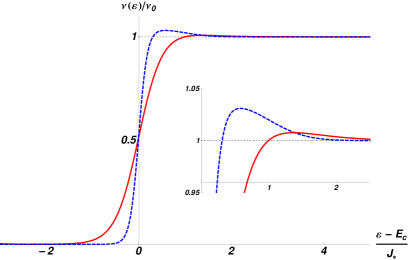
Figure 1: Fig. 1. TDOS in the Coulomb valley. The solid (dashed) line corresponds to $J/\delta=0.92$, $\delta/T=0.35$, and $J_{\star}/T=3.95$ ($J/\delta=0.92$, $\delta/T=0.95$, and $J_{\star}/T=10.70$). The inset depicts the nonmonotonic behavior.

We next consider the average TDOS at $\delta\ll T$. The most interesting regime seems to be that of intermediate temperatures, $T\ll J_{\star}$. Under the assumption $\mu\gg T\ln J_{\star}/T$, Eq. (3) can be simplified, leading to

$$\frac{\overline{\nu}(\varepsilon)}{\nu_{0}}=\sum_{n,\sigma=\pm}e^{-\beta E_{c}(n-N_{0})^{2}}\Biggl{[}\left(1+\frac{J}{2J_{\star}}\right)f_{F}(\sigma\varepsilon-2\sigma\Omega_{n}^{-\sigma})$$

$$-\frac{J}{2J_{\star}}\mathcal{F}\left(\frac{\sigma\varepsilon-2\sigma\Omega_{k}^{\sigma}}{J_{\star}},\beta J_{\star}\right)\Biggr{]}\Biggl{/}\sum_{n}e^{-\beta E_{c}(n-N_{0})^{2}}.$$ (7)

Here $\Omega_{n}^{\sigma}\equiv E_{c}(n-N_{0}+\sigma/2)$, $\nu_{0}$ is the averaged TDOS for noninteracting electrons, and

$$\mathcal{F}(x,y) \equiv \frac{1}{2}\operatorname{sgn}\left(\cos\frac{\pi x}{2}\right)e^{-\frac{y}{4}(x-1)^{2}+\frac{y}{\pi^{2}}\cos^{2}\frac{\pi x}{2}}$$

$$\times \left[1-\Phi\left(\frac{\sqrt{y}}{\pi}\left|\cos\frac{\pi x}{2}\right|\right)\right]+e^{\frac{y}{2}(x-|x|)}$$

$$\times \sum_{m\geqslant 0}(-1)^{m}e^{-y|x|m+ym(m+1)}\theta(|x|-2m-1).$$

$\theta(x)$ is the Heaviside step function ($\theta(0)\equiv 0$), and the error function $\Phi(z)\equiv(2/\sqrt{\pi})\int_{0}^{z}\exp(-t^{2})dt$. As $x$ is varied for a fixed $y$, $\mathcal{F}(x,y)$ exhibits damped oscillations with a period $4$ (equivalent to an energy scale $4J_{\star}$). In the limit $y\gg 1$ considered here, these oscillations are strongly suppressed, and only the first maximum remains visible. It leads to the appearance of a maximum in the TDOS as illustrated in Figs. 1 and 2. The scaling of these oscillations with $\sqrt{\langle S^{2}\rangle}\sim J_{\star}/\delta$ indicates that they are due to precession of the spin of the injected electron about the effective magnetic moment in the dot. This additional structure in the TDOS reflects enhanced electron correlations due to the exchange interaction. At higher temperatures, $T\gg J_{\star}$, there is no interesting signature of spin-exchange on the TDOS.

One can compute the sequential conductance through the QD employing $G=G_{0}\int d\varepsilon(-\partial f_{F}(\varepsilon)/\partial\varepsilon)(\overline{\nu}(\varepsilon)/\nu_{0})$, where $G_{0}$ is the conductance of the non-interacting QD. The maximal value of $G$ will be enhanced by a factor $1+J/2J_{\star}$ due to the exchange term. Much more interestingly, the non-linear conductance at the Coulomb peak will exhibit non-monotonic behavior, similar to Fig.  2  [14].

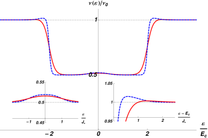
Figure 2: Fig. 2. TDOS at the Coulomb peak. The parameters are the same as in Fig.1. The insets depict the nonmonotonic behavior.

Derivation. - Below we describe the main steps of the derivation. Further details will be given in [14].

The TDOS, $\nu(\varepsilon)=-(1/\pi)\Imag\sum_{\alpha,\sigma}G^{R}_{\alpha\sigma}(\varepsilon)$, is determined via the imaginary part of the retarded Green’s function, $G^{R}_{\alpha\sigma}(t,t^{\prime})=-i\theta(t-t^{\prime})\langle\{a_{\alpha,\sigma}(t),a^{\dagger}_{\alpha,\sigma}(t^{\prime})\}\rangle_{H}$ of the Hamiltonian (2). The imaginary time Green function is given by ${G}_{\alpha\sigma}(\tau_{1},\tau_{2})=-\langle\mathbb{T}_{\tau}\psi_{\alpha,\sigma}(\tau_{1})\bar{\psi}_{\alpha,\sigma}(\tau_{2})\rangle_{S_{\rm tot}}$.

The exact one-particle Green function for the Hamiltonian (2) can be written as

$${G}_{\alpha\sigma}(\tau_{1},\tau_{2})=\int\limits_{-\pi T}^{\pi T}d\phi_{0}\,\frac{\mathcal{Z}(\phi_{0})}{Z}{D}(\tau_{12},\phi_{0})\mathcal{G}_{\alpha\sigma}(\tau_{12},\phi_{0}),$$ (9)

where $\tau_{12}=\tau_{1}-\tau_{2}$, $\phi_{0}$ is the static component of $\phi$, the grand canonical partition function $Z=\int_{-\pi T}^{\pi T}d\phi_{0}\,{D}(0,\phi_{0})\mathcal{Z}(\phi_{0})$, and the so-called Coulomb-boson propagator reads [11, 13]

$$D(\tau,\phi_{0})=e^{-E_{c}|\tau|}\sum_{k\in\mathbb{Z}}e^{i\phi_{0}(\beta k+\tau)-\beta E_{c}(k-N_{0})^{2}-2E_{c}(k-N_{0})\tau}.$$

The one-particle Green function $\mathcal{G}_{\alpha\sigma}(\tau_{1},\tau_{2},\phi_{0})$ appearing in Eq. (9) is defined as $\mathcal{G}_{\alpha\sigma}(\tau_{1},\tau_{2},\phi_{0})=-\langle\mathbb{T}_{\tau}\psi_{\alpha,\sigma}(\tau_{1})\bar{\psi}_{\alpha,\sigma}(\tau_{2})\rangle_{\mathcal{S}}$. Average is taken with respect to the action $\mathcal{S}=\int_{0}^{\beta}d\tau\Bigl{[}\sum_{\alpha}\bar{\Psi}_{\alpha}\partial_{\tau}\Psi_{\alpha}-\mathcal{H}\Bigr{]}$. Here $\mathcal{H}=H_{0}+H_{S}$ with $H_{0}$ in which $\epsilon_{\alpha}$ is replaced by $\tilde{\epsilon}_{\alpha}=\epsilon_{\alpha}-\mu+i\phi_{0}$. Remarkably, the charge and spin degrees of freedom are almost disentangled in the action $\mathcal{S}$. The latter involves only the spin-interaction part of the Hamiltonian (2). Traces of the charging-interaction are encoded in the variable $\phi_{0}$, leading to a small imaginary shift of the chemical potential. Subsequently, the one-particle Green function can be written as

$$\mathcal{G}_{\alpha\sigma}(\tau_{1}>\tau_{2})=-\mathcal{Z}^{-1}\mathcal{K}_{\alpha\sigma}(-i\tau_{12},-i\tau_{12}+i\beta)$$

$$\mathcal{K}_{\alpha\sigma}(t_{+},t_{-})=\operatorname{Tr}e^{-it_{+}\mathcal{H}}a^{\dagger}_{\alpha,\sigma}e^{it_{-}\mathcal{H}}a_{\alpha,\sigma}$$ (10)

and $\mathcal{Z}(\phi_{0})=\operatorname{Tr}\exp(-\beta\mathcal{H})$. In order to evaluate the trace we perform Hubbard-Stratonovich transformations of the terms $e^{\mp it_{\pm}H_{S}}$ in the evolution operators and obtain

$$\mathcal{K}_{\alpha\sigma}(t_{+},t_{-})=\prod_{p=\pm}\int\mathcal{D}[\bm{\theta}_{p}]e^{-\frac{ip}{4J}\int_{0}^{t_{p}}dt^{\prime}\,\bm{\theta}_{p}^{2}}$$ (11)

$$\times\operatorname{Tr}\left[e^{-it_{+}H_{0}}\prod_{\gamma}\mathcal{A}_{\gamma}^{(+)}a^{\dagger}_{\alpha,\sigma}e^{it_{-}H_{0}}\prod_{\eta}\mathcal{A}_{\eta}^{(-)}a_{\alpha,\sigma}\right].$$

Here $\mathcal{A}_{\gamma}^{(p)}$ is defined in Eq. (1). We have defined the bosonic fields $\bm{\theta}_{p}$, $p=\pm$. In order to employ the WNK trick we use a Hamiltonian evolution of our operators rather than a path untegral representation of $\mathcal{G}$. Note that while $\mathcal{H}$ is time independent, the factors $\mathcal{A}_{\gamma}^{(p)}$ involve time ordering ($\mathcal{T}$). This is due to the non-commutativity of the spin-operators $\bm{s}_{\gamma}$.

In order to overcome the intricacy of time-ordering we use the following transformation of variables [16] in the functional integral in Eq. (11) [10],

$$\theta_{p}^{z}=\rho_{p}-2\kappa_{p}^{p}\kappa_{p}^{-p},\,\frac{\theta_{p}^{x}-ip\theta_{p}^{y}}{2}=\kappa_{p}^{-p},$$

$$\frac{\theta_{p}^{x}+ip\theta_{p}^{y}}{2}=-ip\dot{\kappa}_{p}^{p}+\rho_{p}\kappa_{p}^{p}-(\kappa_{p}^{p})^{2}\kappa_{p}^{-p},$$ (12)

which recasts the time-ordered exponent as a product of simple Abelian ones:

$$\mathcal{A}_{\gamma}^{(p)}=e^{p\hat{s}_{\gamma}^{-p}\kappa_{p}^{p}(t_{p})}e^{i\hat{s}_{\gamma}^{z}\int_{0}^{t_{p}}dt^{\prime}\rho_{p}(t^{\prime})}\hskip 71.13188pt{\,}$$ (13)

$$\times\exp\left[i\hat{s}_{\gamma}^{p}\int_{0}^{t_{p}}dt^{\prime}\kappa_{p}^{-p}(t^{\prime})e^{-ip\int_{0}^{t^{\prime}}d\tau\rho_{p}(\tau)}dt^{\prime}\right].$$

Here we employ the initial condition $\kappa_{p}^{p}(0)=0$ [9], and $s_{\gamma}^{\pm}=s_{\gamma}^{x}\pm is_{\gamma}^{y}$. We stress that Eqs. (12) and (13) are valid for a general spin operator. In order to preserve the number of field variables (three) we impose the following constraints on the otherwise arbitrary new complex variables: $\rho_{p}=-\rho_{p}^{*}$ and $\kappa_{p}^{+}=(\kappa_{p}^{-})^{*}$. The quantity $\mathcal{K}_{\alpha\sigma}(t_{+},t_{-})$ can be then evaluated as

$$\mathcal{K}_{\alpha\sigma}(t_{+},t_{-})=\prod_{p=\pm}\int\mathcal{D}[\rho_{p},\kappa_{p}^{p}]e^{-\frac{ip}{4J}\int_{0}^{t_{p}}dt(\rho_{p}^{2}-4ip\dot{\kappa}_{p}^{p}\kappa_{p}^{-p})}$$

$$\times e^{\frac{ip}{2}\int_{0}^{t_{p}}dt\rho_{p}(t)}\mathcal{C}_{\alpha\sigma}(t_{+},t_{-})\prod_{\gamma\neq\alpha}\mathcal{B}_{\gamma}(t_{+},t_{-}),$$ (14)

with $\mathcal{C}_{\alpha\sigma}$ and $\mathcal{B}_{\gamma}$ given in terms of single-particle traces:

$$\mathcal{C}_{\alpha\sigma} = \operatorname{tr}\Bigl{[}e^{-i\varepsilon_{\alpha}\hat{n}_{\alpha}t_{+}}\mathcal{A}_{\alpha}^{(+)}(t_{+})a^{\dagger}_{\alpha\sigma}e^{i\varepsilon_{\alpha}\hat{n}_{\alpha}t_{-}}\mathcal{A}_{\alpha}^{(-)}(t_{-})a_{\alpha\sigma}\Bigr{]},$$

$$\mathcal{B}_{\gamma} = \operatorname{tr}\Bigl{[}e^{-i\varepsilon_{\gamma}\hat{n}_{\gamma}t_{+}}\mathcal{A}_{\gamma}^{(+)}(t_{+})e^{+i\varepsilon_{\gamma}\hat{n}_{\gamma}t_{-}}\mathcal{A}_{\gamma}^{(-)}(t_{-})\Bigr{]}.$$ (15)

The expression for $\mathcal{Z}$ can be obtained from Eq. (14) by the substitution of $\mathcal{B}_{\alpha}$ for $\mathcal{C}_{\alpha\sigma}$. We can now evaluate the single-particle traces in $\mathcal{B}_{\gamma}$ and $\mathcal{C}_{\alpha\sigma}$. The fields $\kappa_{p}^{-}$, $\kappa_{p}^{+}$ appear in $\mathcal{B}_{\gamma}$. It turns out that the integration over $\kappa_{p}^{p}$ first, and then $\rho_{p}$, can be performed exactly, yielding $K_{\alpha\uparrow}(=K_{\alpha\downarrow})$,

$$\mathcal{K}_{\alpha\uparrow}=\frac{e^{-\frac{\beta J}{4}-2i\varepsilon_{\alpha}t_{+}}}{J\sqrt{\pi\beta J}}\int\limits_{-\infty}^{\infty}dh\sinh(\beta h)\prod_{\gamma\neq\alpha}\prod_{\sigma=\pm}\left[1+e^{\beta(\sigma h-\varepsilon_{\gamma})}\right]$$

$$\times\sum_{s=\pm}e^{i\varepsilon_{\alpha}t_{s}+\frac{isJt_{s}}{4}}e^{-\frac{(2\beta h+isJt_{s})^{2}}{4\beta J}}(2\beta h+isJt_{-s}).$$ (16)

Next, we perform the integration over $h$ in Eq. (16), substitute it into Eq. (10) and calculate the exchange-only Green function, $\mathcal{G}_{\alpha\sigma}$. Then, integrating over $\phi_{0}$ in Eq. (9) we obtain the full Green’s function ${G}_{\alpha\sigma}$. Employing the general expression [18]

$$\nu(\varepsilon)=-\frac{2}{\pi}\cosh\frac{\beta\varepsilon}{2}\sum\limits_{\alpha}\int\limits_{-\infty}^{\infty}dt\,e^{i\varepsilon t}G_{\alpha\uparrow}\left(it+\frac{\beta}{2}\right),$$ (17)

we, finally, find the TDOS (3). In a similar way we obtain the partition function $Z$ (4).

Within WNK method one may still have some freedom in selecting regularization of the functional integrals. It is thus useful to check the validity of our results against some benchmarks. Our non-trivial checks are: i) Eq.(5) for $Z$ agrees with the exact derivation in Ref. [5]. ii) The TDOS (3) satisfies the sum rule: $\int d\varepsilon\,\nu(\varepsilon)f_{F}(\varepsilon)=T\partial\ln Z/\partial\mu$ [17]. iii) For $J=0$ our results for the TDOS coincide with those of Ref. [13]. iv) Our results for $Z$ and $\nu(\varepsilon)$ agree with a direct calculation for single and double level QDs.

In summary, we have addressed here the interplay of charging and spin-exchange interactions of electrons in a metallic quantum dot. Even within the simple Universal Hamiltonian framework, this problem leads to a non-Abelian action, and necessarily requires the evaluation of non-trivial time-ordered integrals. Our method is applicable to the vicinity of the Stoner instability (well inside the mesoscopic Stoner unstable regime), and could be extended to the ferromagnetic regime. Other extensions include the study of anisotropic spin-exchange (where the non-vanishing a.c. susceptibility, absorption and TDOS are of particular interest), cotunneling conductance, and an explicit inclusion of the leads.

As a demonstration of the usefulness of our exact solution we have calculated several quantities: the partition function, the magnetic susceptibility, the distribution function of the spin, the TDOS, and the linear and non-linear conductance at the Coulomb peak. Some of these quantities are amenable to experimental tests. Examples: the broad distribution of the spin would imply significant sample-to-sample fluctuations of the measured susceptibility; the latter can be used to determine the distance $(1-J/\delta)$ from the Stoner instability; the relative magnitude of the predicted non-monotonicities in the TDOS and the conductance may exceed $~{}5-10\%$ in materials close to the Stoner instability such as Pd ($J/\delta=0.83)$ or YFe₂Zn₂₀ ($J/\delta=0.94$)  [8].

Previously, Alhassid et al. have calculated exactly the partition function, matrix elements of $a^{\dagger}_{\alpha\sigma},a_{\alpha\sigma}$ [5], and many-body eigenstates which are also eigenstates of the total spin operator [19]. That approach could be employed for the calculation of other observables. Our independent approach is more manageable for the calculation of higher correlators, the inclusion of exchange anisotropy, as well as to further generalizations, as indicated above.

We acknowledge useful discussions with I. Aleiner and V.Gritsev. We thank Y. Alhassid for explaining to us his method and the results of his analysis. We are grateful to I. Kolokolov for providing us with notes of his calculations and a detailed explanation. This work was supported by RFBR Grant No. 09-02-92474-MHKC, the Council for grants of the Russian President Grant No. MK-125.2009.2, the Dynasty Foundation, RAS Programs “Quantum Physics of Condensed Matter”, “Fundamentals of nanotechnology and nanomaterials”, CRDF, SPP 1285 “Spintronics”, Minerva Foundation, German-Israel GIF, Israel Science Foundation, and EU project GEOMDISS.

References

• [1] I. Aleiner, P. Brouwer, and L. Glazman, Phys. Rep. 358, 309 (2002); Y. Alhassid, Rev. Mod. Phys. 72, 895 (2000).
• [2] I.L. Kurland, I.L. Aleiner, B.L. Altshuler, Phys. Rev. B 62, 14886 (2000).
• [3] 50 years of Yang-Mills theory, ed. by G. ’t Hooft, World Scientific, Singapore (2005).
• [4] M.N. Kiselev and Y. Gefen, Phys. Rev. Lett. 96, 066805 (2006).
• [5] Y. Alhassid and T. Rupp, Phys. Rev. Lett. 91, 056801 (2003).
• [6] G. Usaj and H. Baranager, Phys. Rev. B 67, 121308 (2003).
• [7] P. Gambardella et al., Science 300, 1130 (2003); G. Mpourmpakis, G.E. Froudakis, A.N. Andriotis, M. Menon, Phys. Rev. B 72, 104417 (2005).
• [8] S. Jia, S. L. Bud ko, G. D. Samolyuk, P. C. Canfield, Nat. Phys. 3, 334 (2007).
• [9] J. Wei and E. Norman, J. Math. Phys. 4, 575 (1963).
• [10] I.V. Kolokolov, Ann. Phys. (N.Y.) 202, 165 (1990); M. Chertkov and I.V. Kolokolov, Phys. Rev. B 51, 3974 (1994); Sov. Phys. JETP 79, 1063 (1994); for a review see I.V. Kolokolov, Int. J. Mod. Phys. B 10, 2189 (1996).
• [11] A. Kamenev and Y. Gefen, Phys. Rev. B 54, 5428 (1996).
• [12] K.B. Efetov and A. Tschersich, Phys. Rev. B 67, 174205 (2003).
• [13] N. Sedlmayr, I.V. Yurkevich, I.V. Lerner, Europhys. Lett. 76, 109 (2006).
• [14] I. Burmistrov, Y. Gefen, M. Kiselev, and L. Medvedovsky, in preparation.
• [15] M. Schechter, Phys. Rev. B 70, 024521 (2004).
• [16] The Jacobian of the transformation is given as $\mathcal{J}=\prod_{p=\pm}\exp\frac{ip}{2}\int_{0}^{t_{p}}dt\rho_{p}(t)$.
• [17] The sum rule is the consequence of the following relations, $\langle\hat{n}\rangle=-iG^{<}(t,t)$, and $G^{<}(\varepsilon)=2if_{F}(\varepsilon)\Imag G^{R}(\varepsilon)$.
• [18] K.A. Matveev and A.V. Andreev, Phys. Rev. B 66, 045301 (2002).
• [19] H.E. Türeci and Y. Alhassid, Phys. Rev. B 74, 165333 (2006).