Exact Fidelity and Full Fidelity Statistics in Regular and Chaotic Surroundings

Abstract

For a prepared state exact expressions for the time dependent mean fidelity as well as for the mean inverse paricipation ratio are obtained analytically. The distribution function of fidelity in the long time limit and of inverse participation ratio are studied numerically and analytically. Surprising features like fidelity revival and enhanced non–ergodicity are observed. The role of the coupling coefficients and of complexity of background is studied as well.

In quantum information it is crucial to know how well a prepared state can be isolated, and how the unavoidable mixing with the surrounding behaves. The fidelity (often called quantum Loschmidt echo or survival probability) describes how the purity of a prepared state decreases due to the interaction with surrounding states Peres (1984). It serves as a benchmark test of prepared states, e.g. a set of qubits in quantum information Nielsen and Chuang (2000). Of interest is to describe the explicit time-dependence of the fidelity, and how the decay depends on the coupling to the environment, as well as the role played by the complexity of background states. Time-scales, energy scales and explicit shapes of these functions are thus frequently studied Gorin et al. (2006); Jaquod and Petitjean (2009). Survival probability of a state weakly coupled to a background has been subject of considerable research in mesoscopics and in semiclassics Prigodin et al. (1994); Gruver et al. (1997); Vanicek and Cohen (2003); Gutiérrez et al. (2009).

F(ermis) G(olden) R(ule) predicts an exponential decay of the prepared state with decay rate $\Gamma=2\pi\lambda^{2}D$, where $D$ is the mean level spacing of the background and $\lambda$ is the average coupling strength. Deviations from this behavior become important when $\Gamma\simeq D$ Prigodin et al. (1994); Gruver et al. (1997). Corrections to the FGR, which are similar to weak localisation corrections in Quantum Transport can lead to non–ergodicity, i. e.  the prepared state will never decay completelyPrigodin et al. (1994); Gruver et al. (1997).

The observed saturation of fidelity in the long time limit allows us to connect it to the I(nverse) P(articipation) R(atio), which is a time independent quantity. Usually average behavior is considered. But the fidelity in an explicit situation can deviate much from the average behaviorGorin et al. (2004). When constructing quantum information and other devices, requiring high fidelity, one is interested in a high probability to have states with fidelity superior to some minimal value, above which error correction is possible Preskill (1998). In this Letter we therefore study fluctuations of the fidelity and the full fidelity distribution. We find that the latter in the long time limit tends to a stable distribution. This distribution is different from the (time–independent) IPR distribution, both coincide in the weak coupling limit. In this limit we provide an analytical solution. This allows us to study how the distribution depends on coupling strength, coupling type as well as on dynamics of the background.

In addition we provide exact solutions for the mean fidelity for all times and all coupling strength as well as for the mean IPR. We report on nonperturbative features such as a fidelity recovery and enhanced non–ergodicity.

We model the coupling between the prepared state with surrounding complexity by the Hamiltonian

$$H_{\lambda} = H_{s}+H_{b}+\lambda V\ =\ E_{s}|s\rangle\langle s|$$ (1)

$$+\sum_{\nu=1}^{N}E_{\nu}|b_{\nu}\rangle\langle b_{\nu}|+\lambda\sum_{\nu=1}^{N}\left(V_{\nu}|s\rangle\langle b_{\nu}|+h.c.\right).$$

where $H_{s}$ represents a special, pure state, that is coupled to a background of complex states described by $H_{b}$, and where the coupling, $\lambda V$, is controlled by the sortless parameter $\lambda$. Without loss of generality we may put the unperturbed energy of the special state to zero, $E_{s}=0$.

The Schrödinger equations for the uncoupled Hamiltonians are

$$H_{s}|s\rangle=0\mbox{\hskip 19.91692ptand\hskip 19.91692pt}H_{b}|b_{\nu}\rangle=E_{\nu}|b_{\nu}\rangle.$$ (2)

The eigenvalue problem for the coupled Hamiltonian is

$$H_{\lambda}|n\rangle=E_{n}|n\rangle\ .$$ (3)

The $N+1$ eigenfunctions are expressed in a basis of the special state and the background states

$$|n\rangle=c_{ns}|s\rangle+\sum_{\nu=1}^{N}c_{n\nu}|b_{\nu}\rangle,$$ (4)

where $c_{ns}=\langle n|s\rangle$ and $c_{n\nu}=\langle n|b_{\nu}\rangle$. We model the complex surrounding of background states by random matrix theory, and describe generic chaotic states with an ensemble of Gaussian random matrices that can either show time-reversal invariance (GOE, $\beta=1$) or not (GUE, $\beta=2$). Regularity of the background states is modeled by assuming Poisson statistics for $H_{b}$. In all cases the spectrum is unfolded so the mean level spacing equals one, $D=1$, at least in a surrounding of the special state. This implies that the energy scale, including the coupling strength, is always expressed in units of the mean level spacing, while the time scale is expressed in units of the Heisenberg time, $\tau_{H}=\hbar/D$. In the following $\hbar=1$.

Matrix elements of the operator $V$ between the special state and the complex surrounding, $V_{\nu}=\langle s|V|b_{\nu}\rangle$, are taken as Gaussian distributed random numbers with zero mean and variance one. As we will see, it is important to distinguish between real coupling ($V_{\nu}\in{\mathbb{R}}$) and complex coupling ($V_{\nu}\in{\mathbb{C}}$). The size $N$ of the Hilbert space describing the complex surrounding is in principle infinite in RMT. In the numerical simulations it is taken sufficiently large to achieve convergence.

We first focus on fidelity decay. The fidelity amplitude $f_{\lambda}(t)=\langle\Psi_{0}(t)|\Psi_{\lambda}(t)\rangle$ is the overlap, between the pure state, time developed under the influence of the pure Hamiltonian, $|\Psi_{0}(t)\rangle=\exp\left(-i(H_{s}+H_{b})t\right)|\Psi_{0}(0)\rangle$, and under the influence of the perturbed Hamiltonian, $|\Psi_{\lambda}(t)\rangle=\exp\left(-iH_{\lambda}t\right)|\Psi_{0}(0)\rangle$. It is a measure of how the pure initial state, $|\Psi(0)\rangle$, gets disturbed or mixed due to the (unavoidable) coupling to the complex surrounding a time $t$ later. We are interested in the decay of the special state $|s\rangle$, i. e. $|\Psi(0)\rangle=|s\rangle$. We expand it in a basis of eigenstates to $H_{\lambda}$. The fidelity amplitude becomes

$$f_{\lambda}(t)=\sum_{n}|c_{ns}|^{2}\cdot\exp\left(iE_{n}t\right).$$ (5)

It is seen that $f_{\lambda}(t)$ is the Fourier transform of the local density of states (LDOS),

$$\rho(E)=\sum_{n}|c_{ns}|^{2}\delta(E-E_{n}).$$ (6)

The smooth part of the LDOS follows a Breit-Wigner distribution, with the width given by $\Gamma=2\pi\lambda^{2}$, as obtained from FGR under very general assumptions. Therefore the mean fidelity amplitude of the special initial state $|s\rangle$ will unavoidably decay exponentially

$$\overline{f_{\lambda}(t)}=\exp(-\Gamma t/2)\ ,$$ (7)

where the bar denotes average over background and over coupling matrix elements.

The fidelity (survival probability), of the special state is defined as, $F_{\lambda}(t)=|f_{\lambda}(t)|^{2}$. In a Drude–type approximation for the mean fidelity

$$\overline{F_{\lambda}}\ =\ \overline{f_{\lambda}}^{2}=\exp(-\Gamma t)\$$ (8)

FGR is recovered. This result is also obtained by second order perturbation theory. We write fidelity as the sum

$$F_{\lambda}(t)={\rm IPR}+F_{\rm fluc}(t)\ ,$$ (9)

of a constant term and a term which is fluctuating on a timescale comparable to Heisenberg time. The constant term

$${\rm IPR}=\sum_{n}|c_{ns}|^{4}=D\int dE\rho^{2}(E),$$ (10)

is the inverse participation ratio of the special state in the basis of the eigenvectors of the full Hamiltonian. The fluctuating term

$$F_{\rm fluc}(t)\ =\ 2\sum_{n,m}|c_{ns}|^{2}|c_{ms}|^{2}\cos((E_{n}-E_{m})t)$$ (11)

vanishes, if we average fidelity over a time window, large compared with Heisenberg time. Using a Breit–Wigner distribution for $\overline{\rho}(E)$ and the Drude approximation Eq. (8), $\overline{{\rm IPR}_{\lambda}}=D/(\pi\Gamma)$ is found Gruver et al. (1997), which can obviously not hold for small $\Gamma$.

For complex coupling we were able to calculate $\overline{F_{\lambda}(t)}$ exactly for a regular and for a GOE/GUE background. For a regular background the result Kohler et al. (a) is given by

$$\overline{F_{\lambda}(t)} =1+ \frac{\lambda}{2\sqrt{\pi}}\int\limits_{0}^{1}\frac{dx}{\sqrt{x}}e^{-\frac{x\pi^{2}\lambda^{2}}{4(1-x)}}$$ (12)

$$\left\{\frac{\pi}{\sqrt{1-x}}\left(e^{-\frac{t^{2}\lambda^{2}}{x}}\cosh\left(\frac{\pi\lambda^{2}t}{\sqrt{1-x}}\right)-1\right)\right.$$

$$\left.-\frac{2t}{x}e^{-\frac{t^{2}\lambda^{2}}{x}}\sinh\left(\frac{\pi\lambda^{2}t}{\sqrt{1-x}}\right)\right\}\ .$$

For a GUE/GOE background the corresponding more complicated expressions can be found in Kohler et al. (a). For small times this function decays exponentially according to the FGR law. Surprisingly, after some characteristic time fidelity reaches a minimum and increases afterwards to a $\lambda$ dependent saturation value $\overline{F_{\lambda}(\infty)}=\overline{{\rm IPR}_{\lambda}}$. We find for a regular background

$$\overline{{\rm IPR}_{\lambda}} = 1-\frac{\sqrt{\pi}^{3}\lambda}{2}{\rm D}\left(\frac{\pi\lambda}{2}\right)\ ,$$ (13)

with ${\rm D}(\omega)=\exp(\omega^{2}){\rm erfc}(\omega)$. $\overline{{\rm IPR}_{\lambda}}$ is a monotonously decreasing function. For small coupling the saturation value behaves as $\overline{{\rm IPR}_{\lambda}}$ $\simeq$ $1-\pi^{3/2}\lambda$. For large values of $\lambda$ it decays algebraically as $\simeq 2/(\pi^{2}\lambda^{2})$ which is four times the value, obtained by the Drude approximation, Eq. (8). This is a striking enhancement of non–ergodicity. The corresponding expresssion for a GUE background is

$$\overline{F_{\lambda}(\infty)} = 1-\pi^{2}\lambda^{2}-\frac{\sqrt{\pi}^{3}\lambda}{2}\left(1-2\pi^{2}\lambda^{2}\right){\rm D}\left(\pi\lambda\right).$$ (14)

This function decays algebraically as $\simeq 1/(\pi^{2}\lambda^{2})$ for large $\lambda$ which is twice the value, predicted by the Drude approximation.

In Fig.1 fidelity $\overline{F_{\lambda}(t)}$ is plotted for $\lambda=0.1$ for different complexity of the background. For complex coupling the curves are obtained from Eq.(12) respectively from the corresponding expressions taken from Ref. Kohler et al. (a). For real coupling the curves are obtained by Monte Carlo simulations. It is seen that in all three cases fidelity reaches a minimum and saturates afterwards at a finite value. Fidelity decay is stronger for a chaotic background than for a regular background. This is in accordance with the original perturbative arguments by Peres Peres (1984).

Quite remarkably the decay of fidelity is much less sensitive to the complexity of the background than to the structure of the coupling. There is practically no difference between a time reversal invariant chaotic background and a background with broken time–reversal invariance. Nevertheless the difference between a real coupling of the special state to the background and a coupling which breaks time reversal symmetry is sizeable. For one reason, because the return probability from the background into the special state is suppressed by a coupling, which breaks time reversal invariance.

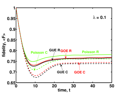
Figure 1: (Color online): Evolution in time of fidelity for coupling strength $\lambda=0.1$. The full lines describe top down fidelity decay for real coupling to a Poissonian (green), to a GOE (red) and to a GUE (black) background. The dashed lines describe top down fidelity decay for complex coupling to a Poissonian (green), to a GOE (red) and to a GUE (blue) background.

We now turn to full fidelity statistics. We introduce the full distribution function

$$P_{\rm F}(c,t)\ =\ \overline{\delta(c-F_{\lambda}(t))}\ .$$ (15)

The distribution of the fidelity $P_{\rm F}(c,t)$ is calculated numerically and plotted for different times in Fig. 2. A saturation of the distribution function is found for times larger than a ($\lambda$–dependent) saturation time. In Fig. 2 this saturation time is about $20$ times Heisenberg time. The saturated distribution is shown in Fig. 3 for GOE statistics and for coupling strength $\lambda=0.05$. It can be compared to the IPR–distribution

$$P_{\rm IPR}(c)\ =\ \overline{\delta\left(c-\sum_{n}|c_{ns}|^{4}\right)}\ .$$ (16)

We see that the two distributions are similar but different. The reason lies in the fluctuating term $F_{\rm fluc}$ (see Eq. (9)). Although the ensemble average of $\overline{F_{\rm fluc}}$ vanishes, its variance does not. Ultimately $F_{\rm fluc}(t)$ contributes substantially to the full fidelity distribution. As a result the stable fidelity distribution and IPR distribution are different.

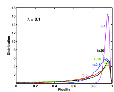
Figure 2: (Color online): Fidelity distributions at times $t=1$ (pink), $t=2.5$ (blue), $t=5$ (red), $t=10$ (green) and $t=20$ (black) for coupling strength $\lambda=0.1$. For times $t>20$ the distribution is stable.

We are interested mainly in cases of high fidelity, that is, when the coupling strength, $\lambda$, is small. In this limit $P_{\rm F}(c,\infty)$ should be better and better approximated by $P_{\rm IPR}(c)$. In this limit an analytic result for $P_{\rm IPR}(c)$ can be obtained. By solving the Schrödinger equations (2) and (3) an expression for the component of the special state in the eigenstates $|n\rangle$ of $H_{\lambda}$ is obtained as

$$|c_{ns}|^{2}=\left(1+\lambda^{2}\sum_{\mu=1}^{N}\frac{|V_{\nu}|^{2}}{(E_{n}-E_{\mu})^{2}}\right)^{-1}.$$ (17)

This exact expression for the components contains eigenvalue solutions, $E_{n}$, as well as input matrix elements $V_{\nu}$ and energies $E_{\nu}$. For small $\lambda$ we may approximate the exact eigenvalues $E_{n}$ by their unperturbed value $E_{\nu(n)}$. If we denote by $|0\rangle$ the eigenstate of $H_{\lambda}$ which has evolved from the special state $|s\rangle$, we see that in this approximation all $|c_{ns}|$ but $|c_{0s}|$ vanish. This means that for small couplings the IPR will be dominated by only one term $|c_{0s}|^{4}$. We define the distribution

$$P_{0}(c)\ =\ \overline{\delta\left(c-|c_{0s}|^{4}\right)}\ .$$ (18)

Then for small $\lambda$, $P_{\rm F}(c,\infty)$ $\simeq$ $P_{\rm IPR}$ and likewise $P_{\rm IPR}$ $\simeq P_{0}$. We could perform the ensemble average of $P_{0}$ exactly. For detail of the calculation see Kohler et al. (b). For a regular surrounding (Poisson statistics) we find:

$$P_{0}(c)=\frac{1}{4\sqrt[4]{c^{3}}}\frac{2\lambda a_{\beta}}{(1-\sqrt{c})^{3/2}}\ {\rm e}^{-(\lambda a_{\beta})^{2}\frac{\pi\sqrt{c}}{1-\sqrt{c}}}.$$ (19)

where $a_{1}$ $=\sqrt{2/\pi}$ for real coupling and $a_{2}$ $=\sqrt{\pi/4}$ for complex coupling. For chaotic surrounding we find for time-reversal symmetry (GOE):

$$P_{0}(c)=\frac{1}{4\sqrt[4]{c^{3}}}\sqrt{\frac{\pi^{3}\lambda^{6}c}{2(1-\sqrt{c})^{5}}}\ {\rm e}^{-X_{1}}\left(K_{0}(X_{1})+K_{1}(X_{1})\right)$$ (20)

where $K_{n}$ are modified Bessel functions of second kind. For a chaotic background without time reversal symmetry (GUE) we get:

$$P_{0}(c)\ =\ \frac{1}{4\sqrt[4]{c^{3}}}\sqrt{\frac{2\pi\lambda^{2}}{(1-\sqrt{c})^{3}}}\ {\rm e}^{-X_{2}}(1+2X_{2}),$$ (21)

with $X_{\beta}$ $=$ $\frac{\beta^{2}\pi^{2}\lambda^{2}\sqrt{c}}{4(1-\sqrt{c})}$ . In Fig. 3 we compare the analytical expressions for the distribution $P_{0}$ to numerical simulations of $P_{\rm IPR}$ and of $P_{\rm F}(c,\infty)$ for $\lambda=0.05$ in the case of a GOE background. We observe good agreement of the analytically calculated $P_{0}(c)$ with the distribution $P_{\rm IPR}(c)$ obtained by simulations. Both curves are indistinguishable at least in the range $c\geq 0.6$. There is a small but notable difference to the distribution $P_{\rm F}(c,\infty)$, which vanishes if we go to smaller values of $\lambda$.

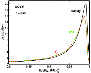
Figure 3: (Color online): Comparison of the distributions $P_{0}$ obtained from Eq. (20) (dashed red line) with $P_{\rm IPR}$ (full green line) and $P_{\rm F}(c,\infty)$ (full black line) obtained from Monte–Carlo simulations for a coupling constant $\lambda=0.05$.

In conclusion, we studied fidelity decay for a special state coupled to a regular or chaotic environment. We found a saturation in the long time limit and a revival. In Prosen and Znidaric (2005) a fidelity freeze was predicted. For a purely off–diagonal perturbation, after an initial decay fidelity freezes on a plateau for some time and decays afterwards to zero. In the model considered here, the perturbation $V$ is purely off–diagonal as well. The saturation, we found here might thus be considered an extreme case of fidelity freeze. The fidelity revival found here is genuinely different to the one reported earlier Stöckmann and Schäfer (2004). There, a satisfactory explanation was given by the spectral rigidity of the GUE/GOEStöckmann and Schäfer (2004); Kohler et al. (2008). The fact that the revival occurs for a regular background as well encumbers such an explanation in the present case.

The saturation of fidelity is a direct consequence of the fact that the fidelity distribution relaxes in the long time limit into a stable distribution. In the small coupling limit it becomes the distribution of the IPR. In this limit we found an analytic expression. Both distributions have a rich structure and are highly sensitive to even small changes in the coupling strength. Their relation to maximum strength distribution, introduced recently Bogomolny et al. (2006); Åberg et al. (2008) will be discussed elsewhere Kohler et al. (b). Their calculation for arbitrary coupling strength is a challenge for the future.

Our results yield an important benchmark for the decay of a prepared quantum state. It might be probed numerically and experimentally in chaotic quantum systems Feist et al. (2006); Bäcker et al. (2008a, b) or on quantum information devices. One instance for a possible numerical experiment is the decay rate of a regular state in a mushroom billiard due to dynamical tunnelling into the chaotic part of the phase space.