A Note on a Certain Non-Gaussian Integral

Abstract:

In this paper we present a general formula for the inhomogeneous non-Gaussian integral $I_{d}(S_{1},S_{2})=\int dx_{1}\ldots dx_{d}e^{-\frac{1}{2}S_{1}^{2}-S_{2}}$, where $S_{1}$ and $S_{2}$ are symmetric quadratic forms. The solution depends on the eigenvalues of the matrix $A=-iM_{2}M_{1}^{-1}$, where $M_{1}$ and $M_{2}$ are the matrix representations of $S_{1}$ and $S_{2}$ respectively. In the $2$-dimensional case we also give a manifestly $SO(2)$-invariant formulation in terms of invariants of the matrix $A$. An expression for $I(S_{1},S_{2})$ in the infinite-dimensional case is calculated and the solution depends only on the determinants of $M_{1}$ and $M_{2}$. The infinite-dimensional case may be of use in QFT.

1 Introduction

Non-Gaussian integrals with homogeneous symmetric forms of degree three and higher were recently studied in [1] and several low-dimensional cases were solved. In this short note we investigate the non-Gaussian integral

$$I_{d}(S_{1},S_{2})=\int dx_{1}\ldots dx_{d}e^{-\frac{1}{2}S_{1}^{2}-S_{2}},$$ (1)

where $S_{1}$ and $S_{2}$ are symmetric quadratic forms. This is the simplest case of a non-homogeneous, non-Gaussian integral. The problem is simplified by the fact that both $S_{1}$ and $S_{2}$ are quadratic since, as such they can be expressed in terms of matrices. We therefore rewrite the integral $I_{d}$ in the following form

$$I_{d}(S_{1},S_{2}) = \int dx_{1}\ldots dx_{d}e^{-\frac{1}{2}S_{1}^{2}-S_{2}}$$ (2)

$$= \int dx_{1}\ldots dx_{d}e^{-\frac{1}{2}(x^{T}M_{1}x)^{2}-x^{T}M_{2}x}$$

$$= \int dt\int dxe^{-t^{2}/2}e^{-x^{T}M_{2}x+itx^{T}M_{1}x}$$

$$= \int dt\frac{e^{-t^{2}/2}}{\sqrt{det(M_{2}-itM_{1})}}$$

where we have used the well-known result

$$\int dx_{1}\ldots dx_{d}e^{-x^{T}Mx}=\frac{1}{\sqrt{det{M}}}.$$ (3)

In [1], A. Morozov and Sh. Shakirov calculate the integrals in terms of the $SL(d)$-invariants of the homogeneous symmetric form $S$. As it turns out that approach is not the most convenient for the present problem. Instead, we shall rewrite the integral to become a function of the eigenvalues of the matrix $A=-iM_{2}M_{1}^{-1}$, in the following way,

$$I_{d}(S_{1},S_{2}) = \int dt\frac{e^{-t^{2}/2}}{\sqrt{det(M_{2}-itM_{1})}}$$ (4)

$$= \frac{i^{d/2}}{\sqrt{det(M_{1})}}\int dt\frac{e^{-t^{2}/2}}{\sqrt{det\left(t\mathbbm{1}-A\right)}}$$

$$= \frac{i^{d/2}}{\sqrt{det(M_{1})}}\int dt\frac{e^{-t^{2}/2}}{\sqrt{(t-z_{1})\ldots(t-z_{d})}}$$

$$\equiv \frac{i^{d/2}}{\sqrt{det(M_{1})}}J_{d},$$

where $z_{i}$ is the $i$:th eigenvalue of the matrix $A$ and

$$J_{d}=\int dt\frac{e^{-t^{2}/2}}{\sqrt{(t-z_{1})\ldots(t-z_{d})}}.$$ (5)

2 Ward identities

In this section we investigate differential operators that annihilate $J_{d}$. Because of the high symmetry of the integrand they take a rather simple form. For simplicity, let us consider the one-dimensional case, where

$$J_{1}=\int dt\frac{e^{-t^{2}/2}}{\sqrt{t-z}}.$$ (6)

We would like to find an operator which turns the integrand into a full derivative. To that end, consider

$$-z\frac{dJ_{1}}{dz} = \frac{1}{2}\int dt\frac{-ze^{-t^{2}/2}}{(t-z)^{3/2}}$$ (7)

$$= \frac{1}{2}J_{1}-\frac{1}{2}\int dt\frac{te^{-t^{2}/2}}{(t-z)^{3/2}}$$

$$= \frac{1}{2}J_{1}+\frac{3}{4}\int dt\frac{e^{-t^{2}/2}}{(t-z)^{5/2}}$$

$$= \frac{1}{2}J_{1}+\frac{d^{2}J_{1}}{dz^{2}},$$

which is equivalent to

$$\frac{d^{2}J_{1}}{dz^{2}}+z\frac{dJ_{1}}{dz}+\frac{1}{2}J_{1}=0.$$ (8)

We have so far not specified the contour of integration in equation 6. It is crucial in the derivation of the Ward identity that the boundary terms vanish. To that end we only consider closed contours. In analogy with [1] we denote an admissible contour as a contour for which the integral 6 converges. In this case any contour that tends asymptotically to the lines $Arg(z)=0$ and $Arg(z)=\pi$ are admissible. To make the integrand single-valued we introduce a branch cut along the line $Arg(z)=0$ as indicated in figure 1. Note that the contours shown in figure 1 are closed on the Riemann sphere if the infinitely remote point is taken into account.

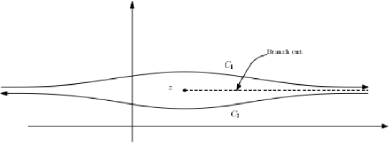
Figure 1: Contour of integration.

There are two classes of admissible contours, and these classes are separated by the branch cut. The fact that there are two essentially different contours means that there will be two different solutions to the integral 6. This can also be seen from that fact that the differential equation 8 is second order. We denote the two independent solutions by $J_{1}^{0}$ and $J_{1}^{1}$.

An equally simple analysis for the $d$-dimensional case gives the following PDE:s:

$$\frac{\partial^{2}J_{d}}{\partial z_{k}^{2}}+\sum_{i\neq k}\frac{\partial^{2}J_{d}}{\partial z_{k}\partial z_{i}}+z_{k}\frac{\partial J_{d}}{\partial z_{k}}+\frac{1}{2}J_{d}=0,$$ (9)

where $k=1,\ldots,d$. In the $d$-dimensional case we have to distinguish between the cases when $d$ is even or odd. The explanation for this is that when $d$ is odd, the integrand of equation 5 has a branch point in the infinitely remote point, whereas in the even-dimensional case the eigenvalues $z_{i}$ are the only branch points. To see this, set $t=\frac{1}{z}$ and $z_{i}=\frac{1}{\alpha}_{i}$ in the denominator of 5:

$$w=\frac{1}{\sqrt{(t-z_{1})\ldots(t-z_{d})}}=\frac{\sqrt{\alpha_{1}\ldots\alpha_{d}}z^{d/2}}{\sqrt{(z-\alpha_{1})\ldots(z-\alpha_{d})}}.$$ (10)

When $z$ is close to the origin, $w$ tends to

$$w=re^{in\theta/2},$$ (11)

which shows that the origin is a branch point in the $z$-plane if and only if $d$ is odd. This in turn means that the infinitely remote point is a branch point for the integrand in equation 5 if and only if $d$ is odd.

Figure 2: Branch cuts for the even-dimensional case.

In order to get a single-valued integrand, we must cut the plane to prevent contours to encircle the branch points. This is done by pairwise connecting the branch points with non-intersecting cuts. In the odd-dimensional case we also make a branch cut from one of the eigenvalues $z_{i}$ to the point at infinity. This is illustrated in figure 2 and 3.

Figure 3: Branch cuts for the odd-dimensional case.

In the even-dimensional case, any straight line not crossing any of the branch cuts is admissible if it is parallell to the real axis. In the odd-dimensional case, let $z_{k}$ be the branch point that is connected to the branch point at infinity. The admissble contours in this case are those that tend asymptotically to the lines $Arg(z_{k})=0$ and $Arg(z_{k})=\pi$ and does not cross any of the other branch cuts. In this way we get two different classes of contours for the odd-dimensional case. The two classes are separated by the branch cut from $z_{k}$ to the infinitely remote point. For the even-dimensional case there is only one class of admissble contours. The two independent solutions to equation 9 are denoted $J_{d}^{0}$ and $J_{d}^{1}$, where $J_{d}^{1}$ is equal to zero in the even-dimensional case.

3 Solution of the Ward identities

3.1 Special cases

Before we start with the general solution, we comment on some special cases. Consider the case when all the eigenvalues $z_{i}$ are equal to one. This means that $M_{2}=iM_{1}$. Moreover the integral

$$J_{d}(1,\ldots,1)=\int dt\frac{e^{-t^{2}/2}}{(t-1)^{d/2}}$$ (12)

is just a constant so that

$$I_{d}(S_{1},S_{2})=\frac{i^{d/2}}{\sqrt{det(M_{1})}}J_{d}\propto\frac{1}{\sqrt{det(M_{1})}},$$ (13)

which is a direct consequence of the following equation that was proved in [1]

$$\int e^{-S(x_{1},\ldots,x_{d})}dx_{1}\ldots dx_{d}\propto\int f\left(S(x_{1},\ldots,x_{d})\right)dx_{1}\ldots dx_{d}.$$ (14)

Next, we consider the case when all the eigenvalues are equal, i.e. $z_{1}=\ldots=z_{d}=z$. In this case the differential equations 9 reduce to the Kummer-equation,

$$\frac{d^{2}J_{d}}{dz^{2}}+z\frac{dJ_{d}}{dz}+\frac{d}{2}J_{d}=0,$$ (15)

which has the solution

$$J_{d}(z,\ldots,z)=cU\left(\frac{d}{4},\frac{1}{2},\frac{z^{2}}{2}\right)+dM\left(\frac{d}{4},\frac{1}{2},\frac{z^{2}}{2}\right),$$ (16)

where $U(a,b,z)$ and $M(a,b,z)$ are the Kummer $U$ and $M$ functions respectively and $c$ and $d$ are constants. Notice that in one dimension this leads to the following well-known result

$$\int ds\frac{e^{-t^{2}/2}}{\sqrt{t-z}}=\frac{1}{\sqrt{2}}\sqrt{z}e^{-z^{2}/4}K_{1/4}\left(\frac{z^{2}}{4}\right),$$ (17)

where $K_{\nu}(z)$ is the modified Bessel-function of the second kind.

3.2 All eigenvalues distinct and non-zero

In this section we solve the differential equations 9 when the eigenvalues of $A$ are distinct and non-zero. The solution is found using Frobenius method, i.e. by assuming the function $J_{d}$ can be expressed by an infinite series,

$$J_{d}=\sum_{i_{1},\ldots,i_{d}=0}^{\infty}a_{i_{1},\ldots,i_{d}}z_{1}^{i_{1}+k_{1}}\ldots z_{d}^{i_{d}+k_{d}},$$ (18)

where the $k_{i}$ are some real numbers to be determined. Since the integral defining the function $J_{d}$ is completely symmetric in its arguments, it is clear that the coefficients $a_{i_{1},\ldots,i_{d}}$ must be completely symmetric in their indices and that $k_{1}=k_{2}=\ldots=k_{d}$, leading to

$$J_{d}=\sum_{i_{1},\ldots,i_{d}=0}^{\infty}a_{i_{1},\ldots,i_{d}}z_{1}^{i_{1}+k}\ldots z_{d}^{i_{d}+k}.$$ (19)

Inserting this expression into equation 9 gives the following algebraic equations

$$a_{i_{1}+2,i_{2},\ldots,i_{d}} = -\frac{i_{2}+k+1}{i_{1}+k+2}a_{i_{1}+1,i_{2}+1,i_{3},\ldots,i_{d}}-\frac{i_{3}+k+1}{i_{1}+k+2}a_{i_{1}+1,i_{2},i_{3}+1,i_{4},\ldots,i_{d}}-\ldots$$ (20)

$$- \frac{i_{d}+k+1}{i_{1}+k+2}a_{i_{1}+1,i_{2},\ldots,i_{d}+1}-\frac{i_{1}+k+1/2}{(i_{1}+k+2)(i_{1}+k+1)}a_{i_{1},\ldots,i_{d}},$$

and

$$k(k-1)=0.$$ (21)

Equation 21 is a consequence of the fact that any second order PDE will be a combination of two linearly independent functions. Note that in even dimension only $k=0$ yields a solution since the integral in this case is invariant under parity (i.e. the transformation $z_{i}\rightarrow-z_{i}$ for all $i$). For $k=0$ we get, after some algebraic manipulations, the following expression for the coefficients

$$a_{i_{1},\ldots,i_{d}} = \frac{(-\frac{1}{2})^{(i_{1}+\ldots+i_{d})/2}\left(\frac{1}{2}\right)_{i_{1}}\ldots\left(\frac{1}{2}\right)_{i_{d}}}{i_{1}!\ldots i_{d}!\left(\frac{d}{4}+\frac{1}{2}\right)_{(i_{1}+\ldots+i_{d})/2}}A_{0},$$ (22)

when $i_{1}+\ldots i_{d}=2n$ and zero otherwise. For $k=1$ they become

$$a_{i_{1},\ldots,i_{d}} = \frac{(-\frac{1}{2})^{(i_{1}+\ldots+i_{d})/2}\left(\frac{3}{2}\right)_{i_{1}}\ldots\left(\frac{3}{2}\right)_{i_{d}}}{(i_{1}+1)!\ldots(i_{d}+1)!\left(\frac{3d}{4}+\frac{1}{2}\right)_{(i_{1}+\ldots+i_{d})/2}}B_{0},$$ (23)

when $i_{1}+\ldots i_{d}=2n$ and zero otherwise. In these formulæ, $(z)_{n}$ is the Pochhammer symbol defined by

$$(z)_{n}=z(z+1)(z+2)\ldots(z+(n-1)).$$ (24)

In summary we have the following expressions for the two independent solutions to equation 9:

$$J_{d}^{0}(z_{1},\ldots,z_{d}) = A_{0}\sum_{i_{1}+\ldots+i_{d}=2n}\frac{(-\frac{1}{2})^{n}\left(\frac{1}{2}\right)_{i_{1}}\ldots\left(\frac{1}{2}\right)_{i_{d}}}{i_{1}!\ldots i_{d}!\left(\frac{d}{4}+\frac{1}{2}\right)_{n}}z_{1}^{i_{1}}\ldots z_{d}^{i_{d}},$$ (25)

and

$$J_{d}^{0}(z_{1},\ldots,z_{d}) = B_{0}\frac{det(M_{2})}{det(M_{1})}\times$$ (26)

$$\times\sum_{i_{1}+\ldots+i_{d}=2n}\frac{(-\frac{1}{2})^{n}\left(\frac{3}{2}\right)_{i_{1}}\ldots\left(\frac{3}{2}\right)_{i_{d}}}{(i_{1}+1)!\ldots(i_{d}+1)!\left(\frac{3d}{4}+\frac{1}{2}\right)_{n}}z_{1}^{i_{1}}\ldots z_{d}^{i_{d}},$$

where $J_{d}^{0}$ corresponds to $k=0$ and $J_{d}^{1}$ to $k=1$. To simplify the notation we set $B_{0}=0$ for $d$ even. The integral $I(S_{1},S_{2})$ is therefore given by

$$I_{d}(S_{1},S_{2})=\frac{1}{\sqrt{det(M_{1})}}\left(J_{d}^{0}+J_{d}^{1}\right).$$ (27)

Taking the limit $d\rightarrow\infty$ only the terms corresponding to $n=0$ survive, leading us to

$$I_{\infty}(S_{1},S_{2})=\frac{1}{\sqrt{det(M_{1})}}\left(A_{0}+\frac{B_{0}det(M_{2})}{det(M_{1})}\right).$$ (28)

3.3 All eigenvalues doubly degenerate and $d$ even

In this section we comment on the special case when $d$ is even and all the eigenvalues of $A$ are doubly degenerate. The differential equations in this case become

$$\frac{\partial^{2}J_{DD}}{\partial z_{k}^{2}}+\sum_{i\neq k}\frac{\partial^{2}J_{DD}}{\partial z_{k}\partial z_{i}}+z_{k}\frac{\partial J_{DD}}{\partial z_{k}}+J_{DD}=0,$$ (29)

where the subscript $DD$ stands for double degeneracy and $k=1,\ldots\frac{d}{2}$. Notice that there are only $\frac{d}{2}$ distinct eigenvalues in this case. We solve these equations in the same way as we did in the previous section, and the result is

$$J_{DD}^{0}(z_{1},\ldots,z_{d/2}) = A_{0}\sum_{i_{1},\ldots,i_{d/2}=2n}\left(-\frac{1}{2}\right)^{n}\frac{1}{\left(\frac{\frac{d}{2}+1}{2}\right)_{n}}z_{1}^{i_{1}}\ldots z_{d/2}^{i_{d/2}}.$$ (30)

Let us look att the first few terms in the sum 30. At the level $n=0$ there is just $A_{0}$. At level $n=1$, we have the following

$$-\frac{2A_{0}}{d+2}\left(z_{1}^{2}+z_{1}z_{2}+z_{1}z_{3}+\ldots\right).$$ (31)

In general at level $n$, we have

$$\left(-\frac{1}{2}\right)^{n}\frac{A_{0}}{\left(\frac{d+1}{2}\right)_{n}}H_{2n}(z_{1},\ldots,z_{d/2}),$$ (32)

where $H_{n}(z_{1},\ldots,z_{d/2})$ is the complete symmetric polynomial of degree $n$ in the variables $z_{i}$. The expressions for the function $J^{0}_{DD}$ can therefore be written

$$J_{DD}^{0}(z_{1},\ldots,z_{d/2}) = A_{0}\sum_{n}\left(-\frac{1}{2}\right)^{n}\frac{1}{\left(\frac{\frac{d}{2}+1}{2}\right)_{n}}H_{2n}(z_{1},\ldots,z_{d/2}),$$ (33)

leaving us with the following simple expression for the integral $I(S_{1},S_{2})$ in this case

$$I_{DD}(S_{1},S_{2}) =\frac{A_{0}}{\sqrt{det(M_{1})}} \sum_{n}\left(-\frac{1}{2}\right)^{n}\frac{H_{2n}(z_{1},\ldots,z_{d/2})}{\left(\frac{\frac{d}{2}+1}{2}\right)_{n}}.$$ (34)

3.4 $SO(d)$-invariance

Even though rewriting the integral $I_{d}(S_{1},S_{2})$ in terms of the eigenvalues of $A=-iM_{2}M_{1}^{-1}$ greatly simplifies the solution, it has the imediate drawback of hiding the $SO(d)$-invariance of $I_{d}(S_{1},S_{2})$. To make this symmetry manifest we must replace the eigenvalues $z_{i}$ with invariants of $A=-iM_{2}M_{1}^{-1}$. In principle this can be done via the Cayley-Hamilton theorem which (in one form) states that

$$(t-z_{1})\ldots(t-z_{d})=t^{d}+I_{1}t^{d-1}+\ldots+I_{d-1}t+I_{d},$$ (35)

where $I_{m}$ are the invariants of $A=-iM_{2}M_{1}^{-1}$. Of course, this is an extremely difficult task except for the low-dimensional cases. In two dimensions we have

$$z_{1} = \frac{1}{2}\left(I_{1}+\sqrt{I_{1}^{2}+4I_{2}}\right),$$

$$z_{2} = \frac{1}{2}\left(I_{1}-\sqrt{I_{1}^{2}+4I_{2}}\right),$$ (36)

so that

$$J_{2}^{0}(I_{1},I_{2}) = A_{0}\sum_{i,j=2n}\frac{(-\frac{1}{2})^{n}\left(\frac{1}{2}\right)_{i}\left(\frac{1}{2}\right)_{j}}{i!j!n!}\times$$ (37)

$$\times\left(\frac{1}{2}\left(I_{1}+\sqrt{I_{1}^{2}+4I_{2}}\right)\right)^{i}\left(\frac{1}{2}\left(I_{1}-\sqrt{I_{1}^{2}+4I_{2}}\right)\right)^{j}.$$

This expression gives the following manifestly $SO(2)$-invariant formulation of $I_{2}(S_{1},S_{2})$:

$$I_{2}(S_{1},S_{2})=\frac{1}{\sqrt{det(M_{1})}}J_{2}^{0}(I_{1},I_{2}).$$ (38)

4 Conclusion and Discussion

In the present paper the non-Gaussian integral

$$I_{d}(S_{1},S_{2})=\int dx_{1}\ldots dx_{d}e^{-\frac{1}{2}S_{1}^{2}-S_{2}}$$ (39)

has been studied. A general formula for any dimension is given in equation 27. The formula is a function of the eigenvalues of the matrix $A=-iM_{2}M_{1}^{-1}$, where

$$S_{1} = x^{T}M_{1}x\mbox{ and}$$

$$S_{2} = x^{T}M_{2}x.$$ (40)

A formula for the infinite-dimensional case is given in equation 28, and depends only on the determinants of $M_{1}$ and $M_{2}$. This formula might be of use in quantum field theory. For two dimensions we give a formula with explicit $SO(2)$-invariance, replacing the eigenvalues with the invariants of $A$. The formulas given in equations 25, 26 and 27 might be of help to calculate the integral discriminant $J_{d|4}$, since any homogeneous action gives an inhomogeneous action when one of the coordinates is replaced by a constant, see equation (3) in [1]. This has not been investigated in the present paper.

References

- [1] A. Morozov and Sh. Shakirov, Introduction to Integral Discriminants, hep-th/09032595
- [2] V. Dolotin, QFT’s With Action of Degree 3 and Higher and Degeneracy of Tensors, hep-th/9706001