Effect of Electric Field on Diffusion in Disordered Materials
II. Two- and Three-dimensional Hopping Transport

Abstract

In the previous paper [Nenashev et al., arXiv:0912.3161] an analytical theory confirmed by numerical simulations has been developed for the field-dependent hopping diffusion coefficient $D(F)$ in one-dimensional systems with Gaussian disorder. The main result of that paper is the linear, non-analytic field dependence of the diffusion coefficient at low electric fields. In the current paper, an analytical theory is developed for the field-dependent diffusion coefficient in three- and two-dimensional Gaussian disordered systems in the hopping transport regime. The theory predicts a smooth parabolic field dependence for the diffusion coefficient at low fields. The result is supported by Monte Carlo computer simulations. In spite of the smooth field dependences for the mobility and for the longitudinal diffusivity, the traditional Einstein form of the relation between these transport coefficients is shown to be violated even at very low electric fields.

I Introduction

This paper represents a second part of our research dedicated to the theory of diffusion of hopping charge carriers biased by electric field in disordered systems with a Gaussian energy distribution of the energy of the localized states:

$$g(\varepsilon)=\frac{N}{\sigma\sqrt{2\pi}}\exp\left(-\frac{\varepsilon^{2}}{2\sigma^{2}}\right),$$ (1)

Here $N$ is the spatial concentration of sites available for hopping transport and $\sigma$ is the energy scale of their density of states (DOS). The Gaussian DOS is assumed to apply for disordered organic materials, such as molecularly doped and conjugated polymers and organic glasses.Roth (1991); Bässler (2000); Pope and Swenberg (1999); Bässler (1993); Borsenberger et al. (1993a); van der Auweraer et al. (1994); Baranovski (2006) While in the previous paper Nenashev et al. (2009) one-dimensional transport was considered, in the current paper we present results for two- and three-dimensional systems. This study has been on one hand stimulated by numerous experimental studies on organic disordered materials,H.-J. Yuh and Stolka (1988); Borsenberger et al. (1991); Borsenberger et al. (1993b); Hirao and Nishizawa (1996, 1997); Lupton and Klein (2002); Harada et al. (2005) which claim the invalidity of the conventional form of the Einstein relation between the carrier mobility $\mu$ and the diffusion coefficient $D$

$$\mu=\frac{e}{kT}D.$$ (2)

On the other hand our study is stimulated by the lack of a concise theory for the diffusion biased by electric field in the hopping transport mode. It is, however, this transport mode that dominates the electrical conduction in disordered organic materials where transport is due to incoherent tunnelling of electrons and holes between localized states randomly distributed in space, with the DOS described by Eq. (1).Roth (1991); Bässler (2000); Pope and Swenberg (1999); Bässler (1993); Borsenberger et al. (1993a); van der Auweraer et al. (1994) The transition rate between an occupied state $i$ and an empty state $j$, separated by the distance $r_{ij}$, is described by the Miller-Abrahams expression Miller and Abrahams (1960)

$$\Gamma_{ij}=\nu_{0}\,e^{-2\frac{r_{ij}}{a}}\left\{\begin{array}[]{ll}e^{-\frac{\Delta\varepsilon_{ij}}{kT}}&,\ \Delta\varepsilon_{ij}>0\\ 1&,\ \Delta\varepsilon_{ij}\leq 0\end{array}\right.,$$ (3)

where $\nu_{0}$ is the attempt-to-escape frequency. The energy difference between the sites is

$$\Delta\varepsilon_{ij}=\varepsilon_{j}-\varepsilon_{i}-Fe(z_{j}-z_{i}),$$ (4)

where the electric field $F$ is assumed to be directed along the $Z$-direction. The localization length of the charge carriers in the states contributing to the hopping transport is $a$. We assume the latter quantity to be independent of energy and we will neglect correlations between the energies of the localized states, following the Gaussian-disorder-model of Bässler. Bässler (1993); Borsenberger et al. (1993a); van der Auweraer et al. (1994); Baranovski (2006)

The field-dependent diffusion in such systems in the 3D case has so far been studied by computer simulations. Richert, Pautmeier, and Bässler performed Monte Carlo simulations in 3D and showed that the longitudinal diffusion coefficient $D_{z}$ is strongly dependent on the electric field and that the dependence is quadratic at such low fields that the mobility of charge carriers remains field-independent.Pautmeier et al. (1991); Richert et al. (1989) This is in contrast to the linear field dependence of the diffusion coefficient at low fields obtained by the exact analytical theory and by numerical calculations for 1D systems in the preceding paper.Nenashev et al. (2009) In order to clarify the nature of the field effect on the diffusion for 3D and 2D systems we suggest in the current paper an analytical theory for the field-dependent diffusion coefficient in the hopping regime for such systems. This theory confirms the conclusion of Richert, Pautmeier, and BässlerRichert et al. (1989); Pautmeier et al. (1991) about the parabolic field dependence of $D_{z}$ at low fields. Furthermore, our theory gives explicit analytical expressions for the combined effects of the electric field and temperature on the hopping diffusion coefficient. These expressions predict a violation of the traditional form of the relation between $\mu$ and $D$ given by Eq. (2) at very low electric fields. Since the temperature effect on the field-dependent diffusion has been so far left out of the scope of computer simulations,Richert et al. (1989); Pautmeier et al. (1991) we perform here a Monte Carlo study of the field- and temperature-dependent diffusion in the hopping regime for 2D and 3D systems in order to check the results of the analytical theory. Our computer simulations for the 2D and 3D cases presented in Sec. II support the analytical theory. Furthermore, numerical results evidence that while the carrier mobility is stable with respect to different realizations of disorder, the diffusion coefficient experiences significant fluctuations from one realization to another, even for systems containing millions of localized states. The reasons for such different behavior between $\mu$ and $D$ is clarified and the estimates for the system size, which is necessary to obtain stable values of $D$, are given in Sec. III.3. The latter estimates show that previous numerical simulations in the literature were performed on rather small systems, insufficient for obtaining reliable results for the field-dependent diffusion coefficient at low temperatures.

In developing the analytical theory for the field-dependent diffusion coefficient for the hopping transport regime we rely on the analogy between the hopping transport mode and the multiple-trapping mode.Orenstein and Kastner (1981); Baranovskii et al. (1997, 2000); Rubel et al. (2004) In Sec. III we present a general solution of the problem. In Sec. IV the analytical expressions from Sec III are compared to simulation results. Concluding remarks are gathered in Sec. V.

II Monte Carlo simulations

In this section we study the effects of field and temperature on the diffusion coefficient by Monte Carlo simulations in more detail than it has been done previously, aiming at a comparison with the analytical theory described in the following sections. Furthermore, we study in detail the role of the system size on the simulated results and show that in order to get reliable results for the field-dependent diffusion at reasonably low temperatures one needs to perform simulations on enormously large systems.

The system is modelled as a lattice of $L^{2}$ or $L^{3}$ sites with lattice constant $d$ and the site energies $\varepsilon_{i}$ chosen randomly according to Eq. (1). Periodic boundary conditions are applied in all directions. Hops inside a square of $7\times 7$ sites (2D case) or a cube of $7\times 7\times 7$ sites (3D case), centered at the starting site are allowed. The simulation proceeds as follows. A packet of $n$ non-interacting carriers is allowed to move in the lattice until a fixed time $t$ has passed. The mobility $\mu$ is calculated from the average distance that the charge carriers have moved along the direction of the field, while the longitudinal diffusion coefficient $D_{z}$ is calculated from the width of the carrier packet:

$$\mu=\frac{\langle z\rangle}{Ft},\qquad D_{z}=\frac{\langle z^{2}\rangle-\langle z\rangle^{2}}{2t}.$$ (5)

Further details of the simulation algorithm and our implementation of it are given in Appendix A. Care was taken about the necessary size of the simulated system in order to avoid finite-size effects. The corresponding number of sites was $700^{3}$ in the 3D case and $15000^{2}$ in the 2D case.

Simulation results for the diffusion coefficient both along and perpendicular to the electric field are shown in Fig. 1, together with the mobility (scaled with $kT/e$). The localization length was $a=0.2d$. A packet consisting of $1000$ charge carriers was simulated for each data point, and the simulation results were averaged over five different realizations of disorder. At extremely low fields it is seen that all three of the plotted quantities are equal, which means that Einstein’s relation, Eq. (2), is valid. With rising magnitude of the electric field the longitudinal diffusion coefficient increases drastically, while the mobility and transversal diffusion coefficient remain field-independent up to much higher fields. The solid line shows a fit to the longitudinal diffusion coefficient by a square trial function

$$D_{z}(F,T)=A(T)F^{2}+D_{0}(T).$$ (6)

It is seen that the square function well fits the data in agreement with the results of previous simulations.Pautmeier et al. (1991)

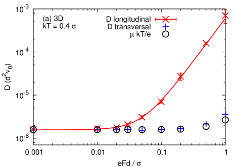
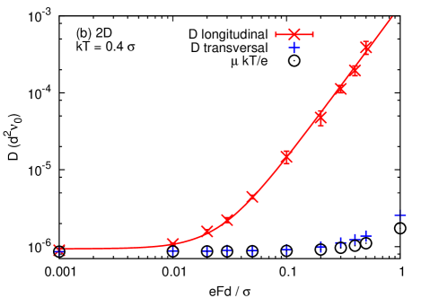
Figure 1: The diffusion coefficient along and perpendicular to the field, and the mobility $\mu$ scaled with $kT/e$ as a function of the field strength, (a) in 3D, and (b) in 2D. At small fields all three quantities are equal, implying that the Einstein relation is valid.

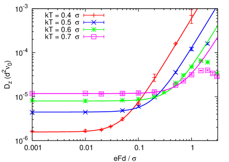
Figure 2: The longitudinal diffusion coefficient $Dz$ for hopping in 3D, as a function of the applied electric field $F$. The solid lines show the best fit to the square function (6).

In order to study the effect of temperature on the field-dependent diffusion coefficient, the simulations were repeated for different temperatures. The results for the longitudinal diffusion coefficient in 3D are collected in Fig. 2. The data are fitted with the square trial functions (6), shown in the figure by solid lines. The fit is good for all temperatures. The decrease of $D_{z}(F)$ at very high fields for the two highest temperatures is due to the trivial saturation effect well-known for the one-dimensional random-energy model.Nenashev et al. (2009) We focus in the following on the field dependence of $D_{z}$ at field magnitudes lower than the one at which $D_{z}$ starts to decrease with increasing field.

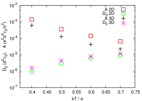
Figure 3: The temperature dependence of $D_{0}$, the diffusion coefficient at $F=0$ and $A$, obtained from Fig. 2 for the localization length $a=0.2d$.

The temperature dependences of the coefficient $A$ in the quadratic field-dependent term for the longitudinal diffusion coefficient $D_{z}$, that were obtained in the 2D and 3D cases by fitting the simulation results in Fig. 2 by Eq. (6) are shown in Fig. 3 along with the field-independent term $D_{0}$. Analytical expressions for $A$ will be derived in Sec. III.

When performing computer simulations for the field-dependent diffusion one should be cautious with the choice of simulation parameters. The field-induced spatial spreading of the carrier packet is caused by trapping of some carriers onto localized states deep in energy, while the other carriers continue their motion in shallow states being biased by the electric field. In order to obtain reliable results for the field-dependent diffusion coefficient, one should guarantee the presence of such deep-in-energy states in the simulated system. Since the DOS given by Eq. (1) rapidly decreases for the deep-in-energy states and hence the sites with deep energies are rare, one has to simulate large systems. The simulation time $t$ must also be chosen so large that the charge carriers have time to visit the deep traps, which control the diffusion. In our simulations $t$ was chosen for each temperature so that the typical number of hops for each carrier was at least $5\cdot 10^{7}$.

The importance of the deep-in-energy states for the field-dependent diffusion is demonstrated in Fig. 4, where the values of $D_{z}$ (at the field $eFd=0.5\sigma$) and of $\mu$ (at low fields) for the temperature $kT=0.33\sigma$ are given when calculated with a cut-off of the DOS below some energy $E_{c}$. For these calculations the normalization of the DOS was kept, while the states with energies below $E_{c}$ were excluded from the simulation. The mobility is almost unaffected by the cutting as long as $E_{c}\lesssim-4\sigma$, while the diffusion coefficient drastically decreases when sites with much smaller energies, around $-6\sigma$, are removed. The result for the mobility $\mu$ is not surprising. It has been predicted in the analytical theoryBaranovskii et al. (2000); Rubel et al. (2004) that the hopping mobility in the Gaussian DOS for the diluted set of carriers is determined by sites with energies in the close vicinity of the average carrier energy $\varepsilon_{\text{av}}=-\sigma^{2}/kT$. For $kT=0.33\sigma$, this energy is $\varepsilon_{\text{av}}\approx-3\sigma$, which explains the data for $\mu$ in Fig. 4. The result for the diffusion coefficient in Fig. 4 shows however that rare sites with even lower energies than $\varepsilon_{\text{av}}$ cause the strong dependence of the diffusion coefficient on the electric field. In Sec. III.3 we show that the most important sites for the field-dependent diffusion have energies around $\varepsilon^{*}=-2\sigma^{2}/kT$, which is much deeper than $\varepsilon_{\text{av}}$. This result also agrees with the data shown in Fig. 4: for $kT=0.33\sigma$, $\varepsilon^{*}\approx-6\sigma$. The diffusion coefficient changes drastically when the few sites with energies below $-5.5\sigma$ are removed, while the mobility starts changing only when $E_{c}$ is in the vicinity of $\varepsilon_{\text{av}}$.

In our simulations a lattice of $700^{3}$ sites has been used. There are typically no sites with energies below $-6\sigma$ in such a system. Therefore, the $D_{z}(F)$ data for $kT=0.33\sigma$ cannot be considered as reliable in the whole simulated range of electric fields. However, for $kT=0.4\sigma$, the lowest temperature considered, $\varepsilon^{*}=-5\sigma$. Energies around $-5\sigma$ are present in our lattice, and thus results for $kT\gtrsim 0.4\sigma$ can be considered as reliable for the lattice of $700^{3}$ sites. It seems extremely lucky that in previous simulations with the lattice of just $70^{3}$ sitesRichert et al. (1989); Pautmeier et al. (1991) meaningful results were claimed for $kT=0.33\sigma$.

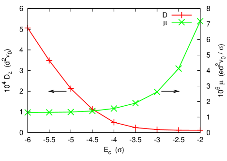
Figure 4: Diffusion coefficient $D_{z}$ (at the field $eFd=0.5\sigma$) and mobility $\mu$ (at low field) in a 3D system where sites with energies below $E_{c}$ are absent. The temperature is $kT=0.33\sigma$.

The analytical results in the preceding paperNenashev et al. (2009) were obtained for nearest-neighbor hopping, while the simulations above allowed also longer hops. To exclude this difference between the models as the cause of the different field dependencies, the simulations for two- and three-dimensional systems were repeated with only nearest-neighbor hopping allowed. The mobility and diffusion coefficient obtained in this case were somewhat lower than those for the variable range hopping, however the parabolic shape of the field dependence for the diffusion coefficient did not change.

Our numerical results can be qualitatively summarized as follows: (i) the diffusion coefficient along the electric field depends parabolically on the field strength $F$ at low fields; (ii) the diffusion coefficient perpendicular to the field is field-independent in the range of fields where Ohm’s law is fulfilled; (iii) the field-dependent part of the diffusion coefficient rapidly decreases with increasing temperature; (iv) the field-dependent part of the diffusion coefficient is very sensitive to sites which energies are lower than the mean carrier energy.

The discussion above, in particular the latter statement on the decisive role of rare sites with very deep energies that can hardly be found in the finite simulation arrays, raises the task of developing an analytical theory for the diffusion process in the hopping regime enhanced by an electric field. There is no such theory in the literature so far. The only relevant theory is the one developed by Rudenko and Arkhipov for band transport in materials with traps.Rudenko and Arkhipov (1982) Although this theory predicts a parabolic field dependence of the longitudinal diffusion coefficient, it cannot be directly applied to hopping transport, because it operates with quantities that are specific for band conductivity (for example, the effective density of states in the conduction band). Therefore it is necessary to develop a theory for hopping transport, particularly because Monte Carlo simulations suffer from finite-size effects as described above. We will give such a theory in Sec. III.

III Analytical results

III.1 Approximation of independent jumps
(general consideration)

The origin of the field-dependent diffusion can be understood qualitatively with the aid of a spatio-temporal picture of the carrier distribution sketched in Fig. 5. The small dots indicate the scatter of carriers after some definite number of jumps, assuming that all carriers start at the same time $t=0$ from the same point. To get the spatial distribution of carriers at some definite time $t^{*}$, one may “project” these dots from the starting point to the line $t=t^{*}$. The direction of “projecting” is determined by the drift velocity. When the drift velocity is equal to zero (no electric field, the left part of Fig. 5), the spatial distribution of carriers at $t=t^{*}$ does not depend on the scatter of times spent by the carriers in order to perform a fixed number of jumps. On the contrary, in the case of drift caused by an electric field (the right part of Fig. 5), this scatter in times “projects” into the line $t=t^{*}$, which gives rise to the broadening of the spatial distribution at $t=t^{*}$. This broadening is the reason for the enhancement of the diffusion coefficient due to electric field.

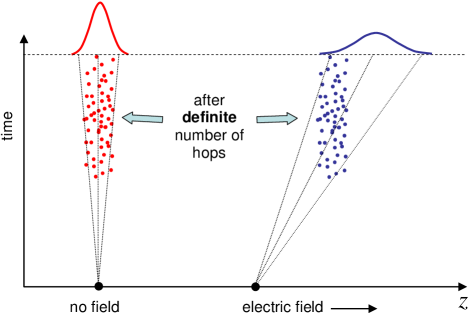
Figure 5: A sketch of spatio-temporal distribution of carriers after some definite number of jumps.

The above consideration shows that fluctuations of the durations of jumps are responsible for the field-induced diffusion. These fluctuations can be especially pronounced for systems with a broad distribution of site energies, because jumps from energetically deep sites to transport sites demand exponentially long times.

Let us start from a general form of the quantitative description for the field dependence of the diffusion coefficient. Our consideration is based on the assumption that successive jumps are statistically independent, i. e. the diffusion process is Markovian. The latter means that increments in carrier coordinates at a given jump, as well as the time interval from the preceding jump till the given one, do not depend on the carrier prehistory. This assumption definitely does not hold for the one-dimensional hopping transport considered in the previous paper.Nenashev et al. (2009) In the 1D case, the probability of returning to an already visited trap is not negligible, and hence the consequent jumps must be correlated. Therefore our analytical consideration based on the assumption of the statistical independence of the successive jumps present below can be valid only for 2D and 3D cases since it is reasonable to assume that in the latter cases the carrier trajectories are non-returning.

Let $t^{*}$ be some fixed moment of time ($t^{*}$ is large compared to the mean time of a jump); $x^{*}$, $y^{*}$ and $z^{*}$ be the carrier’s displacements along the axes $X$, $Y$ and $Z$ during the time interval $[0,t^{*}]$; $x_{1}$, $y_{1}$, $z_{1}$ and $t_{1}$ be coordinate displacements and a time increment related to only one jump, respectively; $x_{n}$, $y_{n}$, $z_{n}$ be the displacements after $n$ successive jumps. Angle brackets will denote averaging over jumps performed by different carriers, equivalent to the averaging over successive jumps of one carrier.

We start with the simple case of zero electric field. Since there is no drift, the expectation values of $x^{*}$, $y^{*}$ and $z^{*}$ vanish, and one obtains for the diffusion coefficients $D_{x}$, $D_{y}$, $D_{z}$

$$D_{x}=\lim_{t^{*}\rightarrow\infty}\frac{\langle x^{*2}\rangle}{2t^{*}},\,D_{y}=\lim_{t^{*}\rightarrow\infty}\frac{\langle y^{*2}\rangle}{2t^{*}},\,D_{z}=\lim_{t^{*}\rightarrow\infty}\frac{\langle z^{*2}\rangle}{2t^{*}}.$$ (7)

For large $t^{*}$, the displacements $x^{*}$, $y^{*}$, $z^{*}$ are approximately equal to $x_{N}$, $y_{N}$, $z_{N}$ – displacements after $N$ jumps, where $N=t^{*}/\langle t_{1}\rangle$ is the mean number of jumps during the time $t^{*}$. Consequently,

$$\frac{\langle x^{*2}\rangle}{2t^{*}}\approx\frac{\langle x_{N}^{2}\rangle}{2t^{*}}=N\frac{\langle x_{1}^{2}\rangle}{2t^{*}}=\frac{\langle x_{1}^{2}\rangle}{2\langle t_{1}\rangle}.$$ (8)

In the limit $t^{*}\rightarrow\infty$ this approximate equality becomes exact, and one gets

$$D_{x}=\frac{\langle x_{1}^{2}\rangle}{2\langle t_{1}\rangle},\quad D_{y}=\frac{\langle y_{1}^{2}\rangle}{2\langle t_{1}\rangle},\quad D_{z}=\frac{\langle z_{1}^{2}\rangle}{2\langle t_{1}\rangle}.$$ (9)

Let us now consider the case of a finite electric field along the $Z$-axis. Since the expectation values of $x^{*}$ and $y^{*}$ are still zero, all the considerations above remain valid, and Eq. (9) remains correct with respect to $D_{x}$ and $D_{y}$. One cannot obtain $D_{z}$ by literally the same way, because $\langle z^{*}\rangle\neq 0$. Instead, one may apply this argumentation to a variable $\tilde{z}=z-vt$, where $v=\langle z_{1}\rangle/\langle t_{1}\rangle$ is the drift velocity. Since $\langle\tilde{z}^{*}\rangle=\langle\tilde{z}_{N}\rangle=\langle\tilde{z}_{1}\rangle=0$, one gets

$$D_{z}\equiv D_{\tilde{z}}\!=\!\!\lim_{t^{*}\rightarrow\infty}\!\!\frac{\langle\tilde{z}^{*2}\rangle}{2t^{*}}\!=\!\frac{\langle\tilde{z}_{1}^{2}\rangle}{2\langle t_{1}\rangle}=\frac{\langle z_{1}^{2}\rangle\!-\!2v\langle z_{1}t_{1}\rangle\!+\!v^{2}\langle t_{1}^{2}\rangle}{2\langle t_{1}\rangle},$$ (10)

and finally

$$D_{z}=\frac{\langle z_{1}^{2}\rangle}{2\langle t_{1}\rangle}-\frac{\langle z_{1}\rangle\langle z_{1}t_{1}\rangle}{\langle t_{1}\rangle^{2}}+\frac{\langle z_{1}\rangle^{2}\langle t_{1}^{2}\rangle}{2\langle t_{1}\rangle^{3}}.$$ (11)

Since the mean values $\langle z_{1}\rangle$, $\langle z_{1}^{2}\rangle$ and $\langle z_{1}t_{1}\rangle$ depend on the electric field, Eq. (11) describes the field-dependent diffusion along the field direction. On the other hand, there is no reason for the mean values $\langle x_{1}^{2}\rangle$, $\langle y_{1}^{2}\rangle$ and $\langle t_{1}\rangle$ to be field-dependent in small electric fields. Therefore, according to Eq. (9), the transversal diffusion coefficients $D_{x}$ and $D_{y}$ are expected to be constant inside the Ohmic regime.

Let us discuss the shape of the dependence $D_{z}(F)$ near the point $F=0$. Since $\langle z_{1}\rangle$ is proportional to the electric field ($\langle z_{1}\rangle=\mu F\langle t_{1}\rangle$, where $\mu$ is mobility), the third term in the r.-h. side of Eq. (11) gives a contribution to $D_{z}(F)$ that is quadratic in $F$. In the first term,

$$\langle z_{1}^{2}\rangle=\langle z_{1}\rangle^{2}+\sigma^{2}[z_{1}],$$ (12)

where $\sigma[a]$ denotes the standard deviation of a random variable $a$. Since $\sigma[z_{1}]$ is not sensitive to the electric field, the first term in the r.-h. side of Eq. (11) is a sum of a constant and a term quadratic in $F$. The behavior of the second term in the r.-h. side of Eq. (11) depends on the symmetry of the system. If in the absence of electric field the directions $Z$ and $-Z$ are equivalent, then $\langle z_{1}t_{1}\rangle=0$ at $F=0$. In this case one expects that $\langle z_{1}t_{1}\rangle\sim F$ and consequently the second term in the r.-h. side of Eq. (11) is quadratic in $F$. However if the positive and negative directions along the $Z$-axis are non-equivalent, $\langle z_{1}t_{1}\rangle$ can be non-zero at $F=0$, which gives a contribution to the diffusion coefficient linear in $F$.

In summary, if the directions $Z$ and $-Z$ are equivalent, which we will assume in the following, the longitudinal diffusion coefficient $D_{z}$ at small fields is described by Eq. (6) where $D_{0}$ and $A$ are field-independent coefficients.

III.2 Multiple-trapping band conductivity

Let us first apply our approach to the multiple-trapping (MT) model of band conductivity. The model includes processes of capture of free carriers by traps, emission of trapped carriers, and free motion (Brownian motion plus drift in the electric field) of carriers in the band (Fig. 6). The band is characterized by the effective density of states $N_{c}$, the mobility $\mu_{f}$ and the diffusion coefficient $D_{f}$ of free carriers. The traps are characterized by the density of states $g(\varepsilon)$ and the capture rate (for unit free carrier concentration) $c(\varepsilon)$. The energy $\varepsilon$ is counted from the band edge.

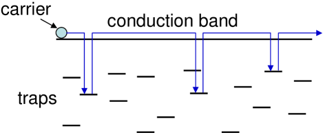
Figure 6: Multiple-trapping conductivity.

The problem of the field-effect on the diffusion coefficient in the MT model has been considered by Rudenko and Arkhipov,Rudenko and Arkhipov (1982) who treated the evolution in time of the one-dimensional carrier distribution function. In Ref. Rudenko and Arkhipov, 1982, transport was assumed to take place in quasi-equilibrium, i. e., the distribution function was assumed to change slowly in comparison with the rate of exchange between traps and the conduction band. Our approach is free of the assumption of quasi-equilibrium transport. Besides, our consideration provides information not only about the longitudinal diffusion coefficient, but also about the transversal one.

Instead of examining the carrier distribution function, we will follow the motion of a single carrier and consider the statistics of this motion. In order to use the expressions (9) and (11), we represent the motion of a carrier as a sequence of “jumps”, each of them beginning at the moment of escape from a trap. Successive “jumps” are statistically independent, because the processes of capture take place in different points in space and there is no correlation between them.

Each “jump” of a carrier consists of two contributions: free motion and sitting on a trap. Let $t_{1f}$ be the time of free motion (between emission and capture), and $t_{1t}$ be the time of being trapped (between capture and emission); $t_{1f}$ and $t_{1t}$ are independent random variables. We denote their expectation values $\langle t_{1f}\rangle$ and $\langle t_{1t}\rangle$ as $T_{1}$ and $T_{2}$, respectively. Since $T_{1}$ is the lifetime of free carriers, its reciprocal value is the capture rate:

$$T_{1}^{-1}=\int c(\varepsilon)g(\varepsilon)d\varepsilon.$$ (13)

The variable $t_{1f}$ obeys an exponential distribution. Hence its mean square $\langle t_{1f}^{2}\rangle$ is equal to $2T_{1}^{2}$.

Collecting all this information, one gets the following statistical expressions for a single “jump” (electric field $F$ is directed along $Z$):

$$\langle t_{1}\rangle =T_{1}+T_{2},$$

$$\langle t_{1}^{2}\rangle =\langle t_{1f}^{2}\rangle+2\langle t_{1f}t_{1t}\rangle+\langle t_{1t}^{2}\rangle=\!2T_{1}(T_{1}+T_{2})+\langle t_{1t}^{2}\rangle,$$

$$\langle x_{1}\rangle =\langle y_{1}\rangle=0,$$ (14)

$$\langle z_{1}\rangle =\mu_{f}F\langle t_{1f}\rangle=\mu_{f}FT_{1},$$

$$\langle x_{1}^{2}\rangle =\langle y_{1}^{2}\rangle=2D_{f}\langle t_{1f}\rangle=2D_{f}T_{1},$$

$$\langle z_{1}^{2}\rangle =\mu_{f}^{2}F^{2}\langle t_{1f}^{2}\rangle+2D_{f}\langle t_{1f}\rangle=2\mu_{f}^{2}F^{2}T_{1}^{2}+2D_{f}T_{1},$$

$$\langle z_{1}t_{1}\rangle =\langle z_{1}t_{1f}\rangle+\langle z_{1}t_{1t}\rangle=2\mu_{f}FT_{1}^{2}+\mu_{f}FT_{1}T_{2}.$$

Using these mean values, one can evaluate the mobility:

$$\mu=\frac{\langle z_{1}\rangle}{F\langle t_{1}\rangle}=\mu_{f}\frac{T_{1}}{T_{1}+T_{2}},$$ (15)

the transversal diffusion coefficient via Eq. (9)

$$D_{x}=D_{y}=\frac{\langle x_{1}^{2}\rangle}{2\langle t_{1}\rangle}=D_{f}\frac{T_{1}}{T_{1}+T_{2}},$$ (16)

and the longitudinal diffusion coefficient via Eq. (11)

$$D_{z}=D_{f}\frac{T_{1}}{T_{1}+T_{2}}+\mu_{f}^{2}F^{2}\frac{T_{1}^{2}\langle t_{1t}^{2}\rangle}{2(T_{1}+T_{2})^{3}}.$$ (17)

The parameters $T_{1}$, $T_{2}$, and $\langle{t}_{1t}^{2}\rangle$ are governed by the capture cross-sections and emission rates of the traps. For moderate electric fields, these cross-sections and rates can be regarded as field-independent, and consequently one can use equilibrium values for $T_{1}$, $T_{2}$, and $\langle{t}_{1t}^{2}\rangle$. This gives an opportunity to simplify Eqs. (15)–(17). The ratio $\alpha\equiv T_{1}/(T_{1}+T_{2})$ contributing to these equations is simply the fraction of free carriers in the equilibrium state. The distribution of the dwell times $\tau$ of a carrier at some individual trap is exponential with the mean value $\langle\tau\rangle=1/\Gamma_{\uparrow}$, where $\Gamma_{\uparrow}$ is the emission rate. Consequently, the mean square of this dwell time is $\langle\tau^{2}\rangle=2\Gamma_{\uparrow}^{-2}$. The mean value $\langle{t}_{1t}^{2}\rangle$ is a weighted average of values $\langle\tau^{2}\rangle$, where the probability of visiting a trap serves as the weight. Therefore,

$$\langle{t}_{1t}^{2}\rangle=\int 2\Gamma_{\uparrow}^{-2}(\varepsilon)p(\varepsilon)d\varepsilon,$$ (18)

where $p(\varepsilon)d\varepsilon$ is the probability of visiting (at a given “jump”) a trap with an energy in the range $[\varepsilon;\varepsilon+d\varepsilon]$:

$$p(\varepsilon)d\varepsilon=\frac{c(\varepsilon)g(\varepsilon)d\varepsilon}{\int c(\varepsilon)g(\varepsilon)d\varepsilon}\equiv T_{1}c(\varepsilon)g(\varepsilon)d\varepsilon.$$ (19)

Expressing the escape rates through capture cross-sections:

$$\Gamma_{\uparrow}(\varepsilon)=c(\varepsilon)N_{c}e^{\varepsilon/kT},$$ (20)

one obtains $\langle{t}_{1t}^{2}\rangle=2T_{1}I$, where

$$I=\int\left(\frac{e^{-\varepsilon/kT}}{c(\varepsilon)N_{c}}\right)^{2}c(\varepsilon)g(\varepsilon)d\varepsilon.$$ (21)

Finally, Eqs. (15)–(17) get the following form:

$$\mu=\alpha\mu_{f},\quad D_{xy}=\alpha D_{f},\quad D_{z}=\alpha D_{f}+\alpha^{3}I\mu_{f}^{2}F^{2},$$ (22)

where $\alpha$ is the equilibrium fraction of free carriers, and $I$ is the integral defined by Eq. (21).

The expressions for $\mu$ and $D_{z}$ are the same as the ones obtained by Rudenko and Arkhipov.Rudenko and Arkhipov (1982) However, our consideration provides some new information about diffusion in the multiple-trapping conductivity regime. First, Eq. (22) shows that the transversal diffusion coefficient is field-independent. Second, we have proven that the equations for $\mu$ and $D_{z}$ are exact (provided that emission/capture probabilities are not influenced by electric field), whereas in Ref. Rudenko and Arkhipov, 1982 they were obtained only under so-called “quasi-equilibrium conditions”.

III.3 Hopping transport

Now we will apply Eq. (11) to two- and three-dimensional hopping transport in a system with a Gaussian DOS, in a manner very similar to our consideration of the multiple-trapping conductivity.

Our analysis is based on the following hypothesis: the field dependence of the diffusion coefficient in 2D and 3D hopping is mainly due to very rare and energetically deep sites. We will call them “traps”. The traps are rare in two senses: first, the typical distance between the traps is large in comparison to the inhomogeneities of the mobility; second, the probability of being trapped is small, so that the traps do not affect the carrier mobility. “Energetically deep” means that the energies of the traps are far below the mean energy of the carriers. We will show below that this hypothesis provides a reasonable description of the Monte Carlo simulation results on the field-dependent diffusion.

As in the previous subsection, we consider the motion of a carrier as a sequence of “jumps”, each beginning when the carrier enters a trap, and ending when the carrier enters another trap. The durations of different “jumps” are not correlated. The same is true for the carrier displacements. Indeed, the three-dimensional Brownian motion is non-returning. This property guarantees that the carrier always visits a new trap, and that the trajectories of its motion between different traps do not overlap. Hence there are no reasons for correlations between successive “jumps”. This is the point where dimensionality is important. In one dimension, the probability of visiting a previously visited trap is not negligible. Consequently the “jumps” must be correlated. Since the “jumps” in the 3D case are not correlated, one can obtain the mobility $\mu$ and the diffusion coefficient $D$ from the statistics of “jumps” using the method of Sec. III.1. For the 2D case we also use the assumption of independent “jumps”.

As in the case of multiple-trapping conductivity, each “jump” consists of two contributions: “free” motion of a carrier and “sitting“ on a trap. Let $t_{1f}$ and $t_{1t}$ be the durations of these contributions; $T_{1}$ and $T_{2}$ denoting the mean values $\langle t_{1f}\rangle$ and $\langle t_{1t}\rangle$, respectively (where averaging is over successive “jumps”); $\mu_{f}$ and $D_{f}$ be the mobility and the diffusion coefficient of “free” motion (energetically far above the traps). With these notations one can follow the same derivation as in the previous subsection and see that Eqs. (15)–(17) are still valid also for hopping transport. It is convenient to rewrite these equations:

$$\mu=\mu_{0},\quad D_{x}=D_{y}=D_{0},\quad D_{z}=D_{0}+AF^{2},$$ (23)

where

$$\mu_{0}=\mu_{f}\frac{T_{1}}{T_{1}+T_{2}},\qquad D_{0}=D_{f}\frac{T_{1}}{T_{1}+T_{2}},$$

$$A=\mu_{0}^{2}\frac{\langle t_{1t}^{2}\rangle}{2(T_{1}+T_{2})}.$$ (24)

In the regime of ohmic conductivity, the values of $\mu_{f}$, $D_{f}$, $T_{1}$, $T_{2}$ and $\langle t_{1t}^{2}\rangle$ can be regarded as field-independent because a sufficiently small electric field does not significantly perturb the probabilities of capture and release. Therefore one can neglect a possible dependence of $\mu_{0}$, $D_{0}$ and $A$ on the electric field. In the following we will use the zero-field values for these quantities.

Let us calculate the coefficient $A$. For convenience, we will consider the system as a large but finite one (with periodic boundary conditions, to allow drift). Then one can obtain the following expressions for $T_{1}$, $T_{2}$ and $\langle t_{1t}^{2}\rangle$:

$$T_{1}=\left(\sum\limits_{t}p_{t}\Gamma_{\text{esc},t}\right)^{-1},$$ (25)

$$T_{2}=T_{1}\sum\limits_{t}p_{t}\,,$$ (26)

$$\langle t_{1t}^{2}\rangle=2T_{1}\sum\limits_{t}p_{t}\Gamma_{\text{esc},t}^{-1}\,,$$ (27)

where the index $t$ runs over all traps, $p_{t}$ is the probability that a carrier is at site $t$, and $\Gamma_{\text{esc},t}$ is the rate of escaping from the trap $t$.

Eq. (25) results from a consideration of the carrier flow from/to traps. Namely, the flow of carriers out of traps is equal to $\sum_{t}p_{t}\Gamma_{\text{esc},t}$; the flow into traps is $T_{1}^{-1}$. In equilibrium, these flows are equal to each other, which gives Eq. (25).

In order to obtain Eqs. (26), (27), we introduce the probability $\mathcal{P}_{t}$ that trap $t$ will be the next visited trap. Let us consider the balance of flows from/to trap $t$. Flow from this trap is equal to $p_{t}\Gamma_{\text{esc},t}$. Flow to it is $\mathcal{P}_{t}T_{1}^{-1}$. Therefore

$$\mathcal{P}_{t}=T_{1}p_{t}\Gamma_{\text{esc},t}.$$ (28)

The mean time of being captured at trap $t$ is $\Gamma_{\text{esc},t}^{-1}$. To obtain $T_{2}$, we average these mean times with corresponding weights $\mathcal{P}_{t}$:

$$T_{2}=\sum\limits_{t}\Gamma_{\text{esc},t}^{-1}\mathcal{P}_{t}\,.$$ (29)

Substituting here Eq. (28), one obtains Eq. (26). Analogously, the mean square of the time of being trapped at site $t$ is $2\Gamma_{\text{esc},t}^{-2}$ (the factor of 2 comes from the exponential distribution of dwell times). Again, we take a weighted average to obtain $\langle t_{1t}^{2}\rangle$:

$$\langle t_{1t}^{2}\rangle=\sum\limits_{t}2\Gamma_{\text{esc},t}^{-2}\mathcal{P}_{t}\,,$$ (30)

that, together with Eq. (28), provides Eq. (27).

The substitution of Eqs. (25)–(27) into Eq. (24) gives the following expression for $A$:

$$A=\mu_{0}^{2}\,\frac{\sum\limits_{t}p_{t}\Gamma_{\text{esc},t}^{-1}}{1+\sum\limits_{t}p_{t}}\,.$$ (31)

Let us try to simplify this expression. The sum in the denominator is the probability that a carrier is at some trap. Due to the rarity of traps, this probability is small, and it can be neglected. The summation in the numerator will be taken over all sites:

$$A\approx\mu_{0}^{2}\sum\limits_{s}p_{s}\Gamma_{\text{esc},s}^{-1}\,.$$ (32)

We will use curly braces to denote the summation in which index $s$ runs over all sites:

$$\{a\}\equiv\sum\limits_{s}p_{s}a_{s},$$ (33)

where $a$ is any quantity specific for sites. It is obvious that curly braces mean averaging over an ensemble of particles (or time averaging, which is the same for finite system and long enough time). Thus,

$$A\approx\mu_{0}^{2}\,\{\Gamma_{\text{esc}}^{-1}\}\,.$$ (34)

Then, the rate of escape $\Gamma_{\text{esc},s}$ is related to the sum $\sum_{s^{\prime}\neq s}\Gamma_{ss^{\prime}}$ of transition rates from site $s$ to any other sites:

$$\Gamma_{\text{esc},s}=n_{\text{esc},s}^{-1}\sum\limits_{s^{\prime}\neq s}\Gamma_{ss^{\prime}}\,,$$ (35)

where $n_{\text{esc},s}$ is the mean number of “attempts” to escape from site $s$ (including the successful one). These “attempts” are events of carrier’s hopping out of site $s$ before the carrier moves so far from this site that it completely forgets the prehistory related to this site. Let us denote the sum $\sum_{s^{\prime}\neq s}\Gamma_{ss^{\prime}}$ as $t_{s}^{-1}$. Then one can rewrite $A$ as

$$A\approx\mu_{0}^{2}\,\{n_{\text{esc}}t\}\,,$$ (36)

or, introducing the averaged number of escape attempts $\overline{n_{\text{esc}}}$,

$$A\approx\overline{n_{\text{esc}}}\,\mu_{0}^{2}\,\{t\}\,.$$ (37)

Calculating $\{t\}$ implies averaging over site energies ($\varepsilon_{s}$) and over quantities related to the neighborhood (energies of neighbors $\varepsilon_{s^{\prime}}$ and distances to them $r_{ss^{\prime}}$). It is possible to treat these two kinds of averaging separately, using our assumption that “optimal” traps are deep in energy. Since the traps are deep, each hop from a trap is upward in energy. Therefore the Miller-Abrahams rates, Eq. (3), for such hops can be written as

$$\Gamma_{ss^{\prime}}=\nu_{0}\exp\left(-\frac{2r_{ss^{\prime}}}{a}+\frac{\varepsilon_{s}-\varepsilon_{s^{\prime}}}{kT}\right).$$ (38)

The dependence of this expression on $\varepsilon_{s}$ has the form of a factor $\exp(\varepsilon_{s}/kT)$. Hence, the quantity $t_{s}=(\sum_{s^{\prime}}\Gamma_{ss^{\prime}})^{-1}$ can be factorized (only for deep sites $s$) as

$$t_{s}=\tau_{s}\,\exp(-\varepsilon_{s}/kT),$$ (39)

where $\tau_{s}$ does not depend on $\varepsilon_{s}$:

$$\tau_{s}=\nu_{0}^{-1}\,\left[\sum\limits_{s^{\prime}\neq s}\exp\left(-\frac{2r_{ss^{\prime}}}{a}-\frac{\varepsilon_{s^{\prime}}}{kT}\right)\right]^{-1}.$$ (40)

Since there are no correlations between $\exp(-\varepsilon_{s}/kT)$ and $\tau_{s}$, one can average these quantities separately:

$$\{t\}\approx\{e^{-\varepsilon_{s}/kT}\tau_{s}\}=\{e^{-\varepsilon_{s}/kT}\}\,\tau.$$ (41)

Here $\tau$ is the mean value of $\tau_{s}$ (an arithmetical average over all $s$). Now, the calculation of $\{e^{-\varepsilon_{s}/kT}\}$ is simple. Remember that $p_{s}$ is an equilibrium probability of finding a carrier at site $s$:

$$p_{s}=\frac{e^{-\varepsilon_{s}/kT}}{\sum\limits_{s^{\prime}}e^{-\varepsilon_{s^{\prime}}/kT}}.$$ (42)

Therefore

$$\{e^{-\varepsilon_{s}/kT}\}\equiv\sum\limits_{s}p_{s}e^{-\varepsilon_{s}/kT}=$$ (43)

$$\frac{\sum\limits_{s}e^{-2\varepsilon_{s}/kT}}{\sum\limits_{s^{\prime}}e^{-\varepsilon_{s^{\prime}}/kT}}=\frac{\int e^{-2\varepsilon/kT}g(\varepsilon)d\varepsilon}{\int e^{-\varepsilon/kT}g(\varepsilon)d\varepsilon}.$$ (44)

For a Gaussian DOS $g(\varepsilon)$ given by Eq. (1), one obtains

$$\{e^{-\varepsilon_{s}/kT}\}=\exp\left(\frac{3\sigma^{2}}{2(kT)^{2}}\right).$$ (45)

Hence

$$\{t\}\approx\tau\exp\left(\frac{3\sigma^{2}}{2(kT)^{2}}\right).$$ (46)

Substituting this result into Eq. (37), one obtains

$$A\approx\overline{n_{\text{esc}}}\,\mu_{0}^{2}\,\tau\exp\left(\frac{3\sigma^{2}}{2(kT)^{2}}\right).$$ (47)

This equation contains $\tau$. The proper way to calculate $\tau$ is the numerical one: to generate at random a large enough number of neighborhoods of the given site (i. e. sets of energies $\varepsilon_{s^{\prime}}$ of neighboring sites and distances $r_{ss^{\prime}}$ from the given site $s$), to calculate $\tau_{s}$ for each neighborhood according to Eq. (40), and then to average the results for $\tau_{s}$. In the next section we compare Eq. (47) to the results of Monte Carlo simulations from Sec. II.

Let us now reveal which traps are “optimal” in the sense that they determine the diffusion coefficient. The integrand in the numerator of Eq. (44) has a sharp peak of width $\sigma$ at $\varepsilon=-2\sigma^{2}/kT$. Hence the “optimal” traps are sites with energies in the range $-2\sigma^{2}/kT\pm\sigma$.

It is now possible to justify our assumption about the possibility to distinguish between the transport sites and the traps. We restrict ourselves to the case of low temperatures, $kT\ll\sigma$. The typical energy of the “optimal” traps, $-2\sigma^{2}/kT$, is significantly lower that the mean energy of carriers $\{\varepsilon\}=-\sigma^{2}/kT$ (the difference is much larger than $kT$). Herewith the assumption that traps are deep in energy is fulfilled. The probability for a carrier to have an energy lower than $-2\sigma^{2}/kT$ is $\sim\exp(-\sigma^{2}/2(kT)^{2})$. This value is much smaller than unity. Therefore neglecting the sum in the denominator of Eq. (31) is justified. Let us now find the typical distance $L_{t}$ between “optimal” traps. Their concentration can be estimated as the concentration of sites with energies lower than $-2\sigma^{2}/kT$, which is about $\sim N\exp(-2\sigma^{2}/(kT)^{2})$, where $N$ is the total concentration of sites. Hence $L_{t}\sim N^{-1/3}\exp(2\sigma^{2}/3(kT)^{2})$. We should compare it to the characteristic size $L_{\mu}$ of inhomogeneities of the mobility. One can estimate this size as a typical distance between sites that are important for the mobility. These are sites with energies close to the mean energy of carriers,Baranovskii et al. (2000); Rubel et al. (2004) $-\sigma^{2}/kT$. Their concentration is about $N\exp(-\sigma^{2}/2(kT)^{2})$. Hence $L_{\mu}\sim N^{-1/3}\exp(\sigma^{2}/6(kT)^{2})$. Herewith we obtain the strong inequality $L_{t}\gg L_{\mu}$, which implies that it is safe to describe the motion of the carriers between traps by means of a constant mobility $\mu_{f}$ and a diffusion coefficient $D_{f}$.

All of the above considerations were based on the Boltzmann statistics for the charge carriers. Let us discuss the effect of the carrier concentration $n$ on the obtained results. The usage of Boltzmann statistics is justified if the Fermi level $\varepsilon_{F}$ is far below the energies of the sites that make a major contribution to the mean value $\{t\}$. As described above, the main contribution to $\{t\}$ comes from sites with energies in the vicinity of $-2\sigma^{2}/kT$. A simple calculation shows that carrier concentration $n_{\text{diff}}$ corresponding to a Fermi level $\varepsilon_{F}=-2\sigma^{2}/kT$ is

$$n_{\text{diff}}\approx N\exp\left(-\frac{3\sigma^{2}}{2(kT)^{2}}\right),$$ (48)

where $N$ is the concentration of sites. The theory considered above presumes that $n\ll n_{\text{diff}}$. In this limit, the diffusion coefficient does not depend on the carrier concentration. For larger concentrations, $n\gg n_{\text{diff}}$, sites with energies $\approx-2\sigma^{2}/kT$ are essentially occupied. In the latter case they cannot efficiently capture the moving charge carriers and therefore the contribution of such sites to the diffusion process (in particular to $\{t\}$) is suppressed. According to Eq. (37), the field-induced part of the diffusion coefficient $D_{z}(F)-D_{0}$ is proportional to $\{t\}$. Therefore, in the case $n\gg n_{\text{diff}}$, $D_{z}(F)-D_{0}$ decreases with increasing $n$. Detailed consideration of this concentration-dependent diffusion is beyond the scope of the present paper.

We should also note that if the sample contains less than $\sim\exp(2\sigma^{2}/(kT)^{2})$ sites, then the average number of “optimal” traps in the sample is less than 1. One should therefore expect large sample-to-sample variations of $D_{z}(F)-D_{0}$ in this case.

IV Comparison of Monte Carlo and analytical results

In this section we discuss relations between the simulation results described in Sec. II and the analytical expression (47).

There are three quantities in Eq. (47) that are not input parameters of the model: the zero-field mobility $\mu_{0}$, the averaged number of escape attempts $\overline{n_{\text{esc}}}$, and the value of $\tau$. For the mobility, we will use the values taken from our simulations. There is no need for a special discussion of the mobility, because it is a well-studied property of the transport model considered here.Baranovski (2006); Baranovskii et al. (2000); Rubel et al. (2004)

The value of $\tau$ was obtained numerically, as explained in the previous section with respect to Eq. (47). The calculation of $\tau$ is relatively inexpensive (as compared to Monte Carlo simulations of the diffusion) and it can be performed over a wide range of model parameters. For the lattice model used in Sec. II, we have found that the simulated dependence of $\tau$ on model parameters is well fitted by the following expressions in two ($\tau_{2D}$) and three ($\tau_{3D}$) dimensions:

$$\tau_{2D}=\left(\frac{kT}{\sigma}\right)^{1/4}\exp\left(\lambda_{2D}\left(\frac{\sigma}{kT}\right)^{1.7}+\eta_{2D}\right),$$ (49)

$$\tau_{3D}=\exp\left(\lambda_{3D}\left(\frac{\sigma}{kT}\right)^{3/2}+\eta_{3D}\right),$$ (50)

where the coefficients $\lambda$ and $\eta$ depend on the ratio of the localization radius $a$ to the lattice parameter $d$:

$$\lambda_{2D} =-1.12\,(a/d)^{0.2}+0.76,$$

$$\eta_{2D} =2.55\,(d/a)^{0.9}-2.4,$$ (51)

$$\lambda_{3D} =0.27\,\log(d/a)-0.74,$$

$$\eta_{3D} =2.92\,(d/a)^{0.85}-3.28.$$

The error of fitting does not exceed 2.5% within the range of parameters $0.2<kT/\sigma<1$ and $0.2<a/d<0.5$.

Extensive computer simulations are necessary to determine the exact value of $\overline{n_{\text{esc}}}$. Without simulations one can only claim that $\overline{n_{\text{esc}}}$ is a number larger than unity, though not exponentially large as a function of model parameters $kT/\sigma$ and $a/d$. Indeed, it follows from the concept of transport energy,Baranovskii et al. (1997, 2000); Rubel et al. (2004) that the energy of a carrier just after its hop from a trap is close to the transport energy. It means that there is no energetic barrier for moving further away from a trap after the first hop. Therefore it is natural to suppose that, when a carrier has jumped out of a trap the probability of escaping i. e. $(\overline{n_{\text{esc}}})^{-1}$ is comparable to 1.

In order to learn more about $\overline{n_{\text{esc}}}$, we used the values of $\mu_{0}$ and $A$ obtained by Monte Carlo simulations. Substituting the data shown in Fig. 3 into Eq. (47), we have extracted $\overline{n_{\text{esc}}}$ for different temperatures in the range $0.33\sigma\leq kT\leq 0.7\sigma$. The localization radius $a$ was chosen equal to $0.2d$. We have obtained that $\overline{n_{\text{esc}}}$ varies in the range from $4.5$ to $8$ in the 2D system, and in the range from $1.6$ to $3.1$ in the 3D system. Simulations have also shown that the values of $\overline{n_{\text{esc}}}$ do not significantly change when the localization radius is changed from $0.2d$ to $0.5d$. One can see that values of $\overline{n_{\text{esc}}}$ found by simulations are indeed reasonable: they are larger than unity but of that order.

Therefore, the analytical consideration presented in Sec. III.3 reduces the problem of predicting the field effect on diffusion to (i) the evaluation of the zero-field mobility $\mu_{0}$, and (ii) the evaluation of a coefficient $\overline{n_{\text{esc}}}$, which is a slowly varying function of the system parameters $kT/\sigma$ and $a/d$. The mobility can be obtained either from computer simulations (which is a much easier task than simulations of the diffusion), or from the analytical theoryBaranovski (2006); Rubel et al. (2004) and experiments. For the sake of self-consistency, we rely here on the simulation data for the mobility. With respect to $\overline{n_{\text{esc}}}$, the comparison between numerical results and the theory shows that one can consider this coefficient as a constant and nevertheless obtain results that agree with simulations. The appropriate choice of this constant for $a=0.2\,d$ is

$$\overline{n_{\text{esc}}}\,\simeq\left\{\begin{array}[]{l}6.0\quad\mbox{(2D),}\\ 2.3\quad\mbox{(3D).}\\ \end{array}\right.$$ (52)

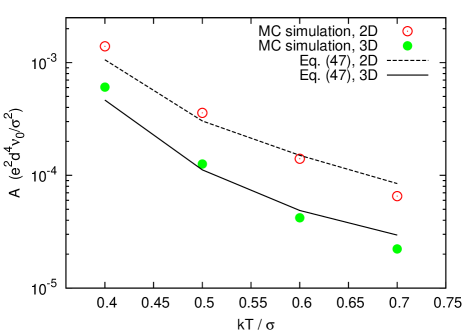
Figure 7: Comparison of Monte Carlo results for coefficient $A$ (symbols) with Eq. (47) (lines) for 2D and 3D transport. Localization length $a=0.2d$. Values of $\tau$ and $\overline{n_{\text{esc}}}$ are taken from Eqs. (49),(50),(52). For $\mu_{0}$ Monte Carlo results are used.

In Fig. 7, Monte Carlo results for the coefficient $A$, which describes the field-induced diffusion according to Eq. (6), are compared to the analytical expression (47). The coefficient $\overline{n_{\text{esc}}}$ in Eq. (47) is set to a constant according to Eq. (52). It is evident that in the framework of the simplifying assumption of constant $\overline{n_{\text{esc}}}$, the analytical theory correctly reproduces the shape of the temperature dependence for the field-induced diffusion coefficient.

V Conclusions

The main result of this paper is the development of an analytical theory for the field-induced diffusion in the hopping transport mode in 3D and 2D systems with the Gaussian DOS given by Eq. (1). At low electric fields, the field dependence of the longitudinal diffusion coefficient $D_{z}(F)$ is parabolic as expressed in Eq. (6). The analytical expression (47) gives the temperature dependence of the field-induced diffusion. Accompanying Monte Carlo simulations confirm the analytical results and show that the shape of the field dependence is parabolic. Together with the exact results of the previous paperNenashev et al. (2009) stating the non-analytic linear field dependence of the diffusion coefficient in the 1D case, our result resolves the long-standing puzzle for the reason of the discrepancies between the analytic and non-analytic behavior of $D_{z}(F)$ claimed in different studiesBouchaud and Georges (1989); Pautmeier et al. (1991): It is the space dimensionality that is responsible for non-analytic (1D) and analytic (2D and 3D) dependences in $D_{z}(F)$.

Furthermore, our theory shows that the main contribution to the field-induced diffusion process comes from localized states with energies in the vicinity of $-2\sigma^{2}/kT$. The DOS parameter $\sigma$ in organic semiconductors is of the order of $0.1$ eV.Pope and Swenberg (1999); Bässler (1993); van der Auweraer et al. (1994); Baranovski (2006) Therefore at room temperatures this energy $-2\sigma^{2}/kT$, which is decisive for $D_{z}(F)$, is situated very deep in the tail of the DOS, around $-8\sigma$. This fact raises very severe demands to the size of the system in computer simulations, which aim at studying the field-induced diffusion in organic semiconductors. In order to have the decisive traps in a simulation at room temperature one needs approximately $10^{16}$ sites. Therefore, such simulations cannot be considered suitable for studying the field-induced diffusion. For instance, the system size of $70^{3}$ used in the previous simulationsPautmeier et al. (1991); Richert et al. (1989) is suitable only at $kT\gtrsim 0.55\sigma$. In contrast, our simulations carried out on systems with $700^{3}$ sites give reliable results at $kT\gtrsim 0.4\sigma$ confirming the developed analytical theory in a wide range of parameters.

In all models the influence of the electric field on the mobility and on the diffusion coefficient increases with decreasing temperature. For the mobility this phenomenon has been accounted in the frame of the concept of the effective temperature.Jansson et al. (2008a, b) The results of this paper show that for the longitudinal diffusion coefficient the concept of the deep traps should be used instead of the effective temperature.

Appendix A Monte Carlo algorithm

For a numerical study of the diffusion in hopping transport, an algorithm is needed that can efficiently simulate transport in large systems. Since the number of sites that can be treated in the simulation is limited by the available memory, we have chosen to study hopping transport on a lattice instead of a system with randomly placed sites.

When the charge carrier is located at site $i$, the probability that the next jump takes it to the site $j$ is given by

$$p_{j}=\frac{\Gamma_{ij}}{\Gamma_{i}},$$ (53)

where $\Gamma_{i}$ is the total rate of hopping away from site $i$:

$$\Gamma_{i}=\sum_{j}\Gamma_{ij}.$$ (54)

The time $\tau$ that the charge carrier spends on the site $i$ before hopping, (the “dwell time”) is calculated as

$$\tau=T/\Gamma_{i},$$ (55)

where $T$ for each hop is randomly generated with an exponential distribution with unit variance. Which jump to perform is decided by picking a random number $x$ between 0 and 1 from a uniform distribution, and finding $j$ such that

$$\sum_{k=1}^{j-1}p_{k}\leq x<\sum_{k=1}^{j}p_{k}$$ (56)

This ensures that each site $k$ is selected with probability $p_{k}$. So far this is the standard Monte Carlo algorithm for hopping transport.Richert et al. (1989); Bässler (1993); Pautmeier et al. (1991) Below an efficient implementation of this algorithm will be described.

Calculating the hopping rates (3) is very time consuming since the exponential function is expensive to compute. If we instead of the site energies $\varepsilon_{i}$ store their exponentials,

$$\kappa_{i}=\exp\left(-\frac{\varepsilon_{i}}{kT}\right),$$ (57)

the hopping rates $\Gamma_{ij}$ can be computed more efficiently. We use the fact that only a small number of discrete displacements are possible for hopping in a lattice, when we restrict the length of the hops. Therefore the geometric part of the hopping rate and the energy contribution from the electric field can be calculated and stored once for each displacement. In our case the hops are restricted to a cube of $7\times 7\times 7$ sites centered at the starting site. For each displacement $\Delta r$, define the quantities

$$\rho_{\Delta r}=\exp\left(-2\frac{\Delta r}{a}\right)$$ (58)

and

$$\varphi_{\Delta r}=\exp\left(\frac{eF\Delta z}{kT}\right),$$ (59)

where $\Delta z$ is the $z$-component of $\Delta r$. The hopping rate from site $i$ to site $j$ located at the position $\Delta r$ relative to $i$ can now be evaluated using

$$\Gamma_{ij}=\nu_{0}\rho_{\Delta r}\min\left(1,\frac{\kappa_{j}}{\kappa_{i}}\varphi_{\Delta r}\right).$$ (60)

One could also consider the storing of all hopping rates $\Gamma_{ij}$, but since this greatly increases the amount of memory needed by the simulation, it would restrict the size of the systems that can be simulated. We have found that a good balance between the simulation speed and the memory requirements is achieved by storing only the rate $\Gamma_{i}$ and the quantity $\kappa_{i}$ for each site, and to calculate the rates $\Gamma_{ij}$ by Eq. (60) during the simulation each time they are needed.

One further optimization is to consider the jumps in order of increasing lengths, since shorter jumps typically have higher probabilities than longer ones. This ordering greatly reduces the number of hopping rates that have to be evaluated before the destination site $j$ that satisfies Eq. (56) is found.

Each carrier was initially placed on a randomly chosen site in the lattice and then allowed to equilibrate before the measurements of time and displacements started.

References

- Baranovski (2006) S. Baranovski, ed., Charge Transport in Disordered Solids with Applications in Electronics (John Wiley & Sons, Ltd, Chichester, 2006).
- Roth (1991) S. Roth, in Hopping transport in solids, edited by M. Pollak and B. I. Shklovskii (Elsevier, 1991), p. 377.
- Bässler (2000) H. Bässler, Semiconducting Polymers, G. Hadziioannou and P. F. van Hutten (eds.) (John Wiley & Sons, Inc., New York, 2000), p. 365.
- Pope and Swenberg (1999) M. Pope and C. E. Swenberg, Electronic Processes in Organic Crystals and Polymers (Oxford University Press, Oxford, 1999).
- Bässler (1993) H. Bässler, Phys. Status Solidi B 175, 15 (1993).
- Borsenberger et al. (1993a) P. M. Borsenberger, E. H. Magin, M. van der Auweraer, and F. C. de Schryver, Phys. Status Solidi A 140, 9 (1993a).
- van der Auweraer et al. (1994) M. van der Auweraer, F. C. de Schryver, P. M. Borsenberger, and H. Bässler, Advanced Materials 6, 199 (1994).
- Nenashev et al. (2009) A. V. Nenashev, F. Jansson, S. D. Baranovskii, R. Österbacka, A. V. Dvurechenskii, and F. Gebhard, arXiv:0912.3161 (2009).
- H.-J. Yuh and Stolka (1988) H.-J. Yuh and M. Stolka, Philos. Mag. B 58, 539 (1988).
- Borsenberger et al. (1991) P. M. Borsenberger, L. Pautmeier, R. Richert, and H. Bässler, Journal of Chemical Physics 94, 8276 (1991).
- Borsenberger et al. (1993b) P. M. Borsenberger, R. Richert, and H. Bässler, Phys. Rev. B 47, 4289 (1993b).
- Hirao and Nishizawa (1996) A. Hirao and H. Nishizawa, Phys. Rev. B 54, 4755 (1996).
- Hirao and Nishizawa (1997) A. Hirao and H. Nishizawa, Phys. Rev. B 56, R2904 (1997).
- Lupton and Klein (2002) J. M. Lupton and J. Klein, Phys. Rev. B 65, 193202 (2002).
- Harada et al. (2005) K. Harada, A. G. Werner, M. Pfeiffer, C. J. Bloom, C. M. Elliott, and K. Leo, Phys. Rev. Lett. 94, 036601 (2005).
- Miller and Abrahams (1960) A. Miller and E. Abrahams, Phys. Rev. 120, 745 (1960).
- Richert et al. (1989) R. Richert, L. Pautmeier, and H. Bässler, Phys. Rev. Lett. 63, 547 (1989).
- Pautmeier et al. (1991) L. Pautmeier, R. Richert, and H. Bässler, Philos. Mag. B 63, 587 (1991).
- Orenstein and Kastner (1981) J. Orenstein and M. Kastner, Solid State Commun. 40, 85 (1981).
- Baranovskii et al. (1997) S. D. Baranovskii, T. Faber, F. Hensel, and P. Thomas, J. Phys. C 9, 2699 (1997).
- Baranovskii et al. (2000) S. D. Baranovskii, H. Cordes, F. Hensel, and G. Leising, Phys. Rev. B 62, 7934 (2000).
- Rubel et al. (2004) O. Rubel, S. D. Baranovskii, P. Thomas, and S. Yamasaki, Phys. Rev. B 69, 014206 (2004).
- Rudenko and Arkhipov (1982) A. I. Rudenko and V. I. Arkhipov, Philos. Mag. B 45, 177 (1982).
- Bouchaud and Georges (1989) J. P. Bouchaud and A. Georges, Phys. Rev. Lett. 63, 2692 (1989).
- Jansson et al. (2008a) F. Jansson, S. D. Baranovskii, G. Sliaužys, R. Österbacka, and P. Thomas, Phys. Status Solidi C 5, 722 (2008a).
- Jansson et al. (2008b) F. Jansson, S. D. Baranovskii, F. Gebhard, and R. Österbacka, Phys. Rev. B 77, 195211 (2008b).