Curvature-driven coarsening in the two dimensional Potts model

Abstract

We study the geometric properties of polymixtures after a sudden quench in temperature. We mimic these systems with the $q$-states Potts model on a square lattice with and without weak quenched disorder, and their evolution with Monte Carlo simulations with non-conserved order parameter. We analyze the distribution of hull enclosed areas for different initial conditions and compare our results with recent exact and numerical findings for $q=2$ (Ising) case. Our results demonstrate the memory of the presence or absence of long-range correlations in the initial state during the coarsening regime and exhibit super-universality properties.

I Introduction

Domains formed during the evolution of mixtures are of both theoretical and technological importance, applications including foams Glazier et al. (1990), cellular tissues Mombach et al. (1993), superconductors Prozorov et al. (2008), magnetic domains Babcock et al. (1990); Jagla (2004), adsorbed atoms on surfaces, etc. In particular, in metallurgy and surface science, the polycrystalline microstructure, and its time evolution, are important in determining the material properties.

After a sudden change in temperature (or in another suitable control parameter) that takes the system from the high temperature phase into the coexistence region, the system tends to organize in progressively larger ordered structures. The system’s temporal evolution is ruled by thermal, diffusive, and curvature driven processes, and the actual growth law depends on general features suchlike the presence of quenched disorder, the dimension of the order parameter and whether it is conserved or not. Although much is known for binary mixtures and systems with twofold ground degeneracy ($q=2$), much less is understood for polymixtures and manifolded ground states ($q>2$). In the latter case, topological defects pin the domain wall dynamics and even in pure systems thermal activation is necessary to overcome the corresponding energy barriers.

Many interesting cellular growth processes are captured by a curvature-driven ordering processes in which thermal effects play a minor role. These are ruled by the Allen-Cahn equation in which the local velocity of an interface is proportional to the local curvature, $v=-(\lambda/2\pi)\kappa$, where $\lambda$ is a temperature and $q$-dependent dimensional constant related with the surface tension and mobility of a domain wall and $\kappa$ is the local curvature. The sign is such that the domain wall curvature is diminished along the evolution. In $d=2$ the time dependence of the area contained within any finite domain interface (the hull) on a flat surface is obtained by integrating the velocity around the hull and using the Gauss-Bonnet theorem:

$$\frac{dA}{dt}=\oint vdl=-\frac{\lambda}{2\pi}\oint\kappa dl=-\lambda\left(1-\frac{1}{2\pi}\sum_{i}\alpha_{i}\right),$$ (1)

where $\alpha_{i}$ are the turning angles of the tangent vector to the surface at the $n$ possible vertices or triple junctions. In some systems, such as the Ising $q=2$ model, $\sum_{i}\alpha_{i}=0$ since there are no such vertices and we obtain $dA/dt=-\lambda$ for all hull-enclosed areas, irrespective of their size Mullins (1956); Arenzon et al. (2007). In highly anisotropic systems, as the Potts model studied here, the angles are all different. In some of the systems that motivate this work, like soap froths, the angles are all equal to $2\pi/3$, that is, $\alpha_{i}=\pi/3,\forall i$. Focusing on systems in which there is a one-to-one correspondence between vertices and sides (meaning that we exclude the Ising limit in which there are no vertices but each wall has one side) the above equation reduces to the von Neumann law von Neumann (1952); Mullins (1956) for the area $A_{n}$ of an $n$-sided hull-enclosed area:

$$\frac{dA_{n}}{dt}=\frac{\lambda}{6}(n-6)\qquad\qquad n>1.$$ (2)

Whether a cell grows, shrinks or remains with constant area depends on its number of sides being, respectively, larger than, smaller than or equal to 6. The above law can be extended to the case in which the typical internal angle depends on the number of sides Glazier and Stavans (1989) and to $3d$ MacPherson and Srolovitz (2007) as well.

Potts models, that is to say $q$-state spin models on a lattice, simulate grain growth. Early studies of the $2d$ $q$-state Potts model with non-conserved order-parameter dynamics have shown that the growth law is analogous to that of the (non conserved) Ising model, where in the scaling regime the characteristic length scale follows the $t^{1/2}$ Allen-Cahn law Grest et al. (1988); Lau et al. (1988), regardless of the value of $q$. However, for $q>2$ and $T=0$, this power law growth does not hold for long times, the characteristic length scale converging to a limiting value. This is in agreement with the Lifshitz-Safran criterium Lifshitz (1962); Safran (1981) that states that when the ground state degeneracy is $q\geq d+1$, where $d$ is the system dimensionality, there might be domain wall pinning depending on the lattice geometry and the density of topological defects. In the $2d$ Potts model Wu (1982) with $q\geq 3$ such point defects are the convergence of three distinct phases borders Lifshitz (1962); Safran (1981). The asymptotic density of defects that depends on $q$ (negligible for $q\leq 4$ but nonzero for $q>4$) was also related with glassy behavior de Oliveira et al. (2004); Ferrero and Cannas (2007). In the presence of thermal fluctuations, the excess energy due to too many domain borders disappears after a transient de Berganza et al. (2007).

In a sequence of papers Arenzon et al. (2007); Sicilia et al. (2007, 2009), we explored the time evolution of domain and hull-enclosed area distributions in bidimensional coarsening systems with scalar order parameter. To study the non-conserved order parameter case, on the one hand we used a continuum description based on the Ginzburg-Landau equation for the scalar field and the Allen-Cahn law $dA/dt=-\lambda$. On the other hand, we studied the kinetic Ising model on a square lattice. For the $q=2$ Ising case with non-conserved order parameter, the absence of triple points leads to the uniform shrinkage of all hull-enclosed areas. More concretely, the number of hull-enclosed areas per unit system area, in the interval $(A,A+dA)$ at time $t$ is related to the distribution at the initial time $t_{i}$ through

$$n_{h}(A,t)=n_{h}\left[A+\lambda(t-t_{i}),t_{i}\right]\;.$$ (3)

Once the initial distribution is known, the above equation gives the distribution at any time $t$. For example, if one takes as initial states at $t_{i}=0$ configurations in equilibrium state at $T_{c}$, where the distribution is exactly known for $q=2$ Cardy and Ziff (2003), $n_{h}(A,0)=c_{h}/A^{2}$ with $c_{h}=8\pi\sqrt{3}$, the distribution at $t>0$ is $n_{h}(A,t)=c_{h}/(A+\lambda_{h}t)^{2}$, that compares extremely well with simulation data for the Ising model on a square lattice Arenzon et al. (2007). For a quench from infinite temperature, on the other hand, the initial distribution corresponds to the one of the critical random continuous percolation Arenzon et al. (2007); Sicilia et al. (2007). This observation is an essential ingredient to understand the fact that, and obtain the probability with which, the system attains a striped frozen state at zero temperature (see Barros et al. (2009) and references therein). Interestingly, on a square lattice, the initial state does not correspond to the random percolation critical point but the coarsening evolution gets very close to it after one or two Monte Carlo steps. Therefore, although Eq. (3) was obtained with the continuous description and, a priori, it is not guaranteed to apply on a lattice, it does describe the coarsening dynamics of the discrete Ising model remarkably accurately. In the presence of vertices, instead, the single hull-enclosed area evolution depends on $n$ and, notably, a given hull-enclosed area can either shrink or grow depending on whether $n<6$ or $n>6$, respectively. Therefore, one cannot write a simple relation as the one in Eq. (3) to link the area distribution at time $t$ to the one at the initial time $t_{i}$ and the distribution might get scrambled in a non-trivial way during the coarsening process (for example, when a domain disappears, the number of sides of the neighboring domains changes, along with their growth rate).

In this paper we study the distribution of hull-enclosed areas during evolution in a Potts model with different number of states, notably $q\leq 4$ and $q>4$. We then try to give an answer to some questions that can be posed when dealing with more than two competing ground states. To what extent the results obtained for $q=2$ are also valid for $q\geq 3$? In particular, in a quench from infinite temperature, does the random percolation critical point affect the evolution as it does for $q=2$? Moreover, which is the interplay between nucleation and growth when the system goes through a first-order phase transition as in the cases $q>4$? What happens when the starting point of the quench is a first order transition point, with finite range correlations? In the presence of weak disorder, when first order transitions become continuous, are the scaling functions universal (super-universality)?

The paper is organized as follows. In section II we introduce the Potts model and, in section III, we study the space-time correlation function starting from differently correlated initial states. Then, in section IV, several area distribution functions, either in the initial state or after the quench in temperature, are studied and described in detail. Afterwards, in section V, the Potts model with ferromagnetic random bonds (weak disorder) is studied and compared with the pure model. Finally, we make some final remarks and conclude.

II The Potts Model

We consider the Potts model Wu (1982) on a square lattice of $N=L^{2}$ spins with $L=10^{3}-5\times 10^{3}$, the state variables of which, $s_{i}$ with $i=1\ldots N$, assume integer values from 1 to $q$. The Hamiltonian is given by

$${\cal H}=-\sum_{\langle ij\rangle}J_{ij}\delta_{s_{i}s_{j}}$$ (4)

where the sum is over nearest-neighbor spins on the lattice and, until section V, $J_{ij}=1,\;\forall i,j$. The transition, discontinuous for $q>4$ and continuous for $q\leq 4$, occurs at $T_{c}=2/\ln(1+\sqrt{q})$. We run from 500 to 4000 Swendsen-Wang (SW) algorithm steps to reach an equilibrium initial condition at the critical point, and average over 1000 samples to build the correlations and distributions. After equilibrium is attained and the system quenched, the evolution follows the heat-bath Monte Carlo algorithm Newman and Barkema (1999) and all times are given in Monte Carlo step (MCs) units, each one corresponding to a sweep over $N$ randomly chosen spins.

\psfrag{r}{$r/R(t)$}\psfrag{cr}{$C(r/R(t))$}\psfrag{t}{$t$}\psfrag{r2}{$R^{2}(t)$}\psfrag{tt}{$t$}\includegraphics[width=256.0748pt]{crtinf2.eps}

Figure 1: (Color online) Rescaled space-time correlation function at several times (from $t=2^{4}$ to $2^{11}$ MCs) after a quench from $T_{0}\to\infty$ to $T_{f}=T_{c}/2$ for $q=2$, 3 and 8, with and without weak disorder (the disordered case is discussed in section V). A good collapse is obtained for all $q$ when rescaling the spatial variable by $R(t)$ obtained from $C(R,t)=0.3$ (note that the working temperature is different in all cases). Inset: $R^{2}(t)$ against $t$ in a double logarithmic scale for $q=2$, 3 and 8 (from top to bottom). The characteristic length, related to the average domain radius, depends weakly on $q$ and $T$ for the pure model (through the prefactor). Within the time window explored there are still some small deviations from the expected Allen-Cahn behavior, $R(t)\simeq t^{1/2}$ in the case $q=8$. When weak disorder is introduced (not shown), the growth rate is greatly reduced and $R^{2}$ deviates from the linear behavior.

After a quench in temperature, the abrupt increase in the local correlation creates an increasing order, despite the competition between different coexisting stable phases. In the cases $q\leq 4$ the paramagnetic state becomes unstable at $T_{c}$ and after a quench to any non-zero sub-critical temperature the system orders locally and progressively in patches of each of the equilibrium phases; in other words, it undergoes domain growth. In the cases $q>4$ one can distinguish three working temperature regimes: at very low $T_{f}$ the system gets easily pinned; at higher $T_{f}$ but below the spinodal temperature $T_{s}$ at which the paramagnetic solution becomes unstable the system undergoes domain growth; above the spinodal $T_{s}$ there is competition between nucleation and growth and coarsening. However, the latter regime is very hard to access since $T_{s}$ is very close to $T_{c}$ (e.g. $T_{s}\simeq 0.95T_{c}$ for $q=96$ Loscar et al. (2009)). In this work we focus on the dynamics in the intermediate coarsening regime.

The detailed evolution of the system during the coarsening dynamics depends on the correlations already present in the initial state, whether absent ($T_{0}\to\infty$), short- ($T_{c}<T_{0}<\infty$ for all $q$ and also $T_{0}=T_{c}$ for $q>4$) or long-range ($T_{0}=T_{c}$ for $q\leq 4$). In the latter case there is already one spanning cluster at $t=0$, since the thermodynamic transition also corresponds to a percolation transition in $2d$. On the other hand, for short-range initial correlations, such spanning domains are either formed very fast (e.g. in the case $q=2$ with $T_{0}\to\infty$), or not formed at all (or at least not within the timescales considered here).

III Equal-time correlations

The degree of correlation between spins is measured by the equal time correlation function

$$C(r,t)=\frac{q}{q-1}\left(\left\langle\delta_{s_{i}(t)s_{j}(t)}\right\rangle_{|i-j|=r}-\frac{1}{q}\right),$$ (5)

where the average is over all pairs of sites a distance $r$ apart. Away from the critical temperature, correlations are short-range, and after a quench from $T_{0}>T_{c}$ to $T_{f}<T_{c}$ these initial correlations become irrelevant after a finite time and the system looses memory of the initial state. In this sense, equilibrium states at all temperatures above $T_{c}$ are equivalent.

Figure 1 shows the correlation function $C(r,t)$ as a function of the rescaled distance, $r/R(t)$, after a quench from infinite temperature, where the initial correlation is null, to a working temperature $T_{f}=T_{c}/2$ for $q=2$, 3 and 8. In the inset, we show the length scale $R(t)$ computed as the distance $r$ at which the correlation has decayed to $0.3$ of its initial value, that is, $C(R,t)=0.3$. The linear behavior $R^{2}\sim t$ is clearly seen for $q=2$. For $q>2$ there are still some deviations from the $t^{1/2}$ law at early times but these disappear at longer times (see also Grest et al. (1988); Lau et al. (1988)). Deviations at short times are indeed expected, due to pinning at low temperatures (note that $T_{f}=T_{c}/2$ decreases with $q$). An excellent collapse of the spatial correlation is observed, as expected from the dynamic scaling hypothesis, when $r$ is rescaled by the length $R(t)$. Moreover, the universal curves seem to coincide for these values of $q$, regardless of the different temperatures after the quench, in accordance with previous evidence Kaski et al. (1985); Kumar et al. (1987); Lau et al. (1988) for the fact that the space-time correlation scaling function (and its Fourier transform, the structure factor) are insensitive to the details of the underlying Hamiltonian. Whether this apparent $q$ independence is only approximate or exact, and in the latter case whether it remains valid for very large values of $q$, are still open issues Liu and Mazenko (1993); Rapapa and Maliehe (2005). As for the Ising model Humayun and Bray (1992), the small $r$ behavior is linear for all $q$, in agreement with Porod’s law Bray (1994); Liu and Mazenko (1993).

\psfrag{r}{$r/R(t)$}\psfrag{cr}{$C(r,t)$}\psfrag{t}{$r$}\psfrag{t4}{$t=4$}\psfrag{t10}{$t=2^{10}$}\psfrag{r2}{$C(r,t)$}\psfrag{r4}{$r^{-1/4}$}\psfrag{tt}{$t^{1/2}$}\includegraphics[width=256.0748pt]{crtc2.eps}

Figure 2: (Color online) Rescaled space-time correlation function at several times ($t=4,\ldots,2^{10}$ MCs) after a quench from $T_{0}=T_{c}$ to $T_{f}=T_{c}/2$ for the Ising $q=2$ case in log-log scale (cfr. Figs. 3 and 4 for $q=3$ and $q=8$, respectively). A very good collapse is obtained when rescaling the spatial variable by $R(t)$, obtained from $C(R,t)=0.7$. At $t=0$, the correlation decays as $r^{-\eta}$ ($\eta=1/4$), while for $t>0$ partial memory of the initial state is preserved, as evidenced by the power-law tail. The inset presents $C(r,t)$ for the same times used in the main figure, with no rescaling of $r$. The correlation at $t=0$ is also shown, and deviations from the power-law behavior are already present, due to the strong fluctuations in magnetization at $T_{c}$.

\psfrag{r}{$r/R(t)$}\psfrag{cr}{$C(r,t)$}\psfrag{t}{$t$}\psfrag{r2}{$R^{2}(t)$}\psfrag{r4}{$r^{-4/15}$}\psfrag{tt}{$t$}\includegraphics[width=256.0748pt]{crtc_q3.eps}

Figure 3: (Color online) Rescaled space-time correlation function at several times ($t=4,\ldots,2^{10}$ MCs) after a quench from $T_{0}=T_{c}$ to $T_{f}=T_{c}/2$ for $q=3$ in log-log scale (cfr. Figs. 2 and 4 for $q=2$ and $q=8$, respectively). The slope $r^{-\eta}$ with $\eta=4/15$ is shown as a guide to the eye. Inset: $R^{2}(t)$ for $q=2$ (top) and 3 (bottom), obtained from $C(R,t)=0.7$ together with the law $R^{2}\simeq t$.

On the other hand, when the starting point is an equilibrium state at $T_{c}$ with long-range correlations ($q\leq 4$) obtained by performing a sufficient number of Swendsen-Wang steps Newman and Barkema (1999), the system keeps memory of the long-range correlations present in the critical initial state. The equal time equilibrium correlation function decays at the critical temperature as a power-law, $C(r,0)\sim r^{2-d-\eta}$, where both the coefficient and the exponent $\eta$ depend on $q$. For example, in two dimensions, $\eta=1/4$ for $q=2$ and $\eta=4/15$ for $q=3$ Wu (1982). Figure 2 shows the rescaled correlation function at several instants after the quench for $q=2$. Some remarks are in order. First, there is a very good collapse for length scales up to $r\sim R(t)$, where $R(t)$ is such that $C(R,t)=0.7$. Second, deviations from the initial power-law occur both at short and long length scales. Due to the ever growing structures, correlations decrease very slowly for small $r$. Indeed, $C$ almost follows the plateau close to unity up to a certain, time increasing, distance. For long distances, on the other hand, these deviations occur because the initial states can be magnetized (at $T_{c}$, magnetization goes as $L^{-\beta/\nu}$) and, as $r$ increases and the spins decorrelate, $C(r,t)$ attains a plateau at $m^{2}(t)$. Since, eventually, the system equilibrates, the longer the time, the larger the magnetization and, consequently, the higher the plateau. Although not done here, it is also possible to postpone the approach to equilibrium by choosing initial states with very small magnetization, as done by Humayun and Bray Humayun and Bray (1991), who also introduced a correction factor to account for boundary effects due to the system size being much smaller than the correlation length, $L\ll\xi$, at $T_{c}$. Essentially the same behavior is obtained for $q=3$ with $\eta=4/15$ (shown in Fig. 3) and $q=4$ with $\eta=1/2$ (not shown), respectively. We obtain the same scaling function for different final temperatures (not shown), indicating that super-scaling holds with relation to temperature.

\psfrag{r}{$r/R(t)$}\psfrag{cr}{$C(r,t)$}\psfrag{tt}{$t$}\psfrag{r2}{$R^{2}(t)$}\psfrag{t}{$t$}\includegraphics[width=256.0748pt]{crtc_q8.eps}

Figure 4: (Color online) Rescaled space-time correlation function at several times ($t=2^{10},\ldots,2^{14}$ MCs) after a quench from $T_{0}=T_{c}$ to $T_{f}=T_{c}/2$ for $q=8$ in linear-linear scale (cfr. Figs. 2 and 3 for $q=2$ and $q=3$, respectively).

For $q>4$, differently from the previous cases, there are no long-range correlations at $T=T_{c}$, only finite-range ones. The actual correlation length at $T_{c}$ can be obtained analytically Buffenoir and Wallon (1993), but we did not attempt to measure it, since the correlator that we use does not remove power-like prefactors Janke and Kappler (1995). For quenches below the limit of stability of the paramagnetic high-temperature state, see Fig. 4 for $q=8$, the finite correlation length at $t=0$ is washed out once the scaling regime is attained. As might have been expected, the scaling function is indistinguishable, within our numerical accuracy, from the one for systems with a continuous phase transition ($q=2,\ 3$) quenched from infinite temperature, cfr. Fig. 1. The collapse is not as good at short times since it takes longer for the system to approach the scaling regime in the $q=8$ case (see the inset).

After some discussion it is now well-established that weak quenched disorder changes the order of the phase transition from first-order to second-order when $q>4$. The critical exponent $\eta$ depends on $q$ although very weakly. The scaling function of the space-time correlation function after a quench from the critical point also depends on $q$ Jacobsen and Picco (2000); d’Auriac and Iglói (2003).

IV Area Distributions

More insight on the growing correlation observed during the coarsening dynamics after the quench can be gained from the study of the different area distributions $n(A,t)$. We consider two measurements: geometric domains and hull-enclosed areas. Geometric domains are defined as the set of contiguous spins in the same state. In principle, such domains may enclose smaller ones that, in turn, may also enclose others and so on. One can also consider the external perimeter of the geometric domains (the hull) and the whole area enclosed by it. Let us discuss the distribution of these areas after a quench from higher to low temperatures.

IV.1 The initial states

Prior to the quench, the system is prepared in an initial state having either zero, finite or infinite range correlation, corresponding to $T_{0}=\infty$ ($\forall q$), $T_{0}=T_{c}$ ($q>4$) and $T_{0}=T_{c}$ ($q\leq 4$), respectively. Infinite temperature states are created by randomly assigning, to each spin, a value between 1 and $q$, while to obtain an equilibrium state at $T_{c}$, the system is further let evolve during a sufficient number of Swendsen-Wang Monte Carlo steps at $T_{c}$ (typically 500).

\psfrag{A}{$A$}\psfrag{log}{$\ln[A\ n_{h,d}(A,0)]$}\psfrag{8}{8}\psfrag{5}{5}\psfrag{4}{4}\psfrag{q=3}{$q=3$}\psfrag{logAn}{$\log An(A,0)$}\includegraphics[width=227.62204pt]{dist_2d_t0.eps}

Figure 5: (Color online) Equilibrium domain (blue triangles) and hull-enclosed area (red squares) distributions at $T_{0}\to\infty$ for several values of $q$, corresponding to the random percolation problem at $1/q$ occupation density. The data are shown in linear-log scale.

IV.1.1 $T_{0}\to\infty$

When the temperature is infinite, neighboring spins are uncorrelated, and the configurations can be mapped onto those of the random percolation model with equal occupation probability $p=1/q$. On the square lattice considered here, this state is not critical for all values of $q$ (criticality would require that one of the species density be $0.59$). The highest concentration of a single species, $0.5$, is obtained for $q=2$. This corresponds to the continuous random percolation threshold but on a lattice, however, it is critical percolation on the triangular case only. Still, for the $q=2$ Ising model on a square lattice, as shown in Arenzon et al. (2007), the proximity with the percolation critical point strongly affects the system’s evolution.

Figure 5 shows the geometric domains and hull-enclosed area distributions $n(A,0)=qn_{\scriptstyle\rm rp}(A,1/q)$, where $n_{\scriptstyle\rm rp}(A,p)$ is the corresponding size distribution for random percolation with occupation probability $p=1/q$. The factor $q$ comes from the fact that the $q$ species equally contribute to the distribution, while in the percolation problem, a fraction $1-1/q$ of the sites is empty. Unfortunately, $n_{\scriptstyle\rm rp}$ is not known analytically for general values of $p$ away from $p_{c}$. For $q=2$ (not shown, see Sicilia et al. (2007)), the system is close to the critical percolation point, and the distributions are power-law, $n(A,0)\simeq A^{-\tau}$ with $\tau=2$ for hull-enclosed areas and $\tau\gtrsim 2$ for domain areas, up to a large area cut-off where they cross over to exponential decays. For $q=3$, deviations from linearity are already perceptible and, moreover, the hull-enclosed and domain area distributions can be resolved. For sufficiently low $p$ (but probably valid for all $p<p_{c}$) the distribution tail is exponential Muller-Krumbhaar and Stoll (1976); Kunz and Souillard (1978); Schwartz (1978); Stoll and Domb (1979); Hoshen et al. (1979); Schmittmann and Bruce (1985) and the simulation data is compatible with Parisi and Sourlas (1981); Stauffer and Aharony (1994) $n_{\scriptstyle\rm rp}(A,p)\sim A^{-\theta}\exp[-f(p)A]$, where the exponent $\theta$ depends on the dimension only ($\theta=1$ for $d=2$). Since all $q$ states are equally present, the domains are typically smaller the larger the value of $q$ and the occupation dependent coefficient $f(p)$ thus increases for increasing $q$ or decreasing $p$. The data for the different distributions shown in Fig. 5 can only be resolved for large values of $A$ and small values of $q$. These differences are due to domains embedded into larger ones, already present in the initial state, that may remain at long times after the quench. For larger values of $q$ the distributions get closer to an exponential in their full range of variation and it becomes harder and harder to distinguish hull-enclosed and domain area probability distribution functions (pdfs).

\psfrag{A}{$A$}\psfrag{nh}{$\displaystyle\frac{n_{h}(A,0)}{q-1}$}\psfrag{nh2}{$\small\frac{n_{h}(A,0)A^{2}}{q-1}$}\psfrag{q10}{$10$}\psfrag{q8}{$q=8$}\includegraphics[width=227.62204pt]{dist_nh_t0.eps}

Figure 6: (Color online) Equilibrium power-law distribution of hull-enclosed areas at $T_{c}$ for several values of $q$, from 2 to 8. The line is $c_{h}^{(2)}/A^{2}$, from Eq. (6). Taking $c_{h}^{(q)}$ as a fitting parameter one finds very small values obeying $c_{h}^{(4)}<c_{h}^{(3)}<c_{h}^{(2)}$ (see text). For $q>4$, the transition is discontinuous but nonetheless the distribution follows the power law until a crossover length, beyond which it decays exponentially, as shown in the inset for $q=8,\ 10$ and, for comparison, $q=2$ (the horizontal data).

IV.1.2 $T_{0}=T_{c}$ and $2\leq q\leq 4$

When the transition is second order and the system is equilibrated at the critical temperature $T_{c}$, the distribution of both domains and hull-enclosed areas follow a power law. For example, for $q=2$ in $d=2$, the hull-enclosed area distribution is given by $n_{h}(A,0)=c_{h}^{(2)}/A^{2}$, where $c_{h}^{(2)}=1/8\pi\sqrt{3}\simeq 0.0229$ Cardy and Ziff (2003). Generally, the hull-enclosed area distribution for $q=2$, 3 and 4, is found to be

$$n_{h}(A,0)=\frac{(q-1)c_{h}^{(q)}}{A^{2}}$$ (6)

as can be seen in Fig. 6. We choose to use the $q-1$ prefactor instead of $q$ for consistency with our previous work. This can be done, however, with a small modification of the constant, $(q-1)c_{h}=qc_{h}^{\prime}$. Thus, each spin species contributes with the same share to the total distribution. Notice that, unless for $q=2$, the value of $c_{h}^{(q)}$ is not known exactly. A rough estimate of the constants can be obtained by taking them as fit parameters; we obtain $c_{h}^{(3)}\simeq 0.0203$ and $c_{h}^{(4)}\simeq 0.0192$. The fit for $q=2$ yields $c_{h}^{(2)}\simeq 0.0227$, that compares well with the exact value. The constants obey the inequality $c_{h}^{(4)}<c_{h}^{(3)}<c_{h}^{(2)}$.

For geometric domains, a relation similar to Eq. (6) is obtained for the area distribution at $T_{c}$ and $2\leq q\leq 4$. The exponent is slightly larger than 2, $\tau=379/187$ for $q=2$ Stella and Vanderzande (1989); Stauffer and Aharony (1994); Sicilia et al. (2007), and seems to be independent of $q$ for $q=3,\ 4$. The coefficients, however, are not exactly known (numerically, for $q=2$, it is close to $c_{h}^{(2)}$ Sicilia et al. (2007)).

IV.1.3 $T_{0}=T_{c}$ and $q>4$

When the transition is discontinuous, the power law exists up to a crossover length, typically of the order of the correlation length $\xi$, where the distribution deviates and falls off faster. Depending on the values of $\xi$ and $L$, the crossover may or may not be observed due to the weakness of the transition. For example, for $q=5$, 6 and 8, estimates Buffenoir and Wallon (1993); Deroulers and Young (2002) of $\xi$ are, 2512, 159 and 24, respectively. For $q=5$, $\xi$ is indeed larger than the system size $L$ that we are using and the system behaves as it were critical. Figure 6 also presents data for the hull-enclosed area distributions in models with $q=6$, 8 and 10, where the deviations from the power-law are very clear, and occurring at smaller values of $A$ for increasing $q$, as expected. Equation (6) is thus valid up to this crossover length. The inset of Fig. 6 shows that for areas that are larger than a certain value $A^{*}_{q}$, the distribution decays exponentially for $q>4$. Thus, the general form of the hull-enclosed area distribution, apparently valid for all values of $q$ at $T_{c}$, is

$$n_{h}(A,0)=\frac{(q-1)c_{h}^{(q)}}{A^{2}}e^{-\alpha_{q}\frac{A}{A^{*}_{q}}}$$ (7)

where $\alpha_{q}=0$ for $q\leq 4$.

The area distribution of geometric domains is very similar to the hull-enclosed area one. None of the coefficients $c_{d}^{(2)}$, are exactly known; the numerical results for $q=2$ described in Sicilia et al. (2007) suggest that $c_{d}^{(q)}$ is very close to $c_{h}^{(2)}$ and the study of the distributions for $q=3,\ 4$ suggests that the similarity between $c_{d}^{(q)}$ and $c_{h}^{(q)}$ holds for general $q$ as well.

IV.2 The coarsening regime

In Fig. 7 we show snapshots of the system at $t=2^{10}$ MCs after the quench for different values of $q$ and $T_{0}$. When the initial condition is equilibrium at $T_{c}$ for $2\leq q\leq 4$, the system presents larger domains than when the initial conditions are random, since the latter has an exponential instead of a power-law size distribution. On the other hand, for $q>4$, when the correlation length at $T_{c}$ is finite, there is no visible difference in the snapshots. In these figures, with the exception of some very small thermally induced fluctuations, there is no domain fully embedded inside another one, at variance with the $q=2$ behavior Sicilia et al. (2007). Nonetheless, in Fig. 8, one such rare embedded domain occurs, being created after a coalescence process among the neighbors. Thus, for $q>2$, due to this shortage of embedded domains (neglecting the small thermal fluctuations), there is little difference between geometric domains and hull-enclosed area measures, implying that the parameters of the distributions should have similar values.

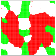
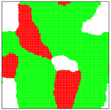
(a)                                   (b)

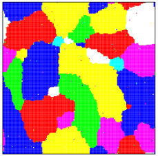
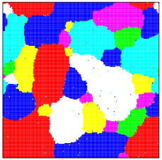
(c)                                   (d)

Figure 7: (Color online) Snapshots at $t=2^{10}$ MCs after a quench from $T_{0}\to\infty$ and $T_{0}=T_{c}$, left and right, respectively to $T_{f}=T_{c}/2$, for $q=3$ [(a) and (b)] and $q=7$ [(c) and (d)]. Different colors correspond to different species. Notice that, for $q=7$, some domains have just coalesced (for example, the large yellow domain in panel (c), an effect that is absent for $q=2$ and becomes rarer as $q$ increases. Figure 8 gives a more detailed view of such occurrence. A few thermal fluctuations are also visible as small dots inside the clusters. Note that the structures are typically larger on the right column ($T_{0}=T_{c}$) than on the left one ($T_{0}\to\infty$) for $q=3$. This is not the case for $q=7$ where there are no big structures in the initial state since $\xi(q=7,T_{c})$ is finite.

\psfrag{t0}{t=500}\psfrag{t1}{600}\psfrag{t2}{700}\psfrag{t3}{800}\includegraphics[width=256.0748pt]{multiplotq3.eps}

Figure 8: (Color online) Snapshots at several times after a quench from $T_{0}\to\infty$ to $T_{f}=T_{c}/2$, for $q=3$. Different colors correspond to the three different species. The snapshots show the coalescence of two white domains inside the $100\times 100$ zoomed region. Notice also the rare occurrence of a domain fully embedded into a single domain at $t=800$ MCs.

IV.2.1 $2<q\leq 4$ and $T_{0}\to\infty$ (finite correlation length)

Despite the existence of many similarities between the Potts model with $q=2,\ 3$ and 4, there are also some fundamental differences. Besides all having a continuous transition, the equal time correlation function seems to share the same universal scaling function and the related correlation length grows with the same power of time, $t^{1/2}$, see Sect. II. Nevertheless, differently from the $q=2$ case, that presents a percolating domain with probability almost one as early as $t=2$ after the quench Arenzon et al. (2007); Sicilia et al. (2007), the $q>2$, $T_{0}\to\infty$ initial condition is sufficiently far from critical percolation that the system remains, at least in the time window of our simulations, distant from the percolation threshold (in spite of the largest domain steadily, but slowly, increasing with time).

As the system evolves after the quench, the distribution keeps memory of the initial state, that corresponds to random percolation with occupation probability $p=1/q$. And, by not getting close to a critical point, the distributions do not become critical and, as a consequence, do not develop a power law tail, as illustrated in Fig. 9 for $q=3$ and $T_{0}\to\infty$. There is, however, an $A^{-2}$ envelope that is a direct consequence of dynamical scaling, present also for other values of $q$. The scaling hypothesis requires that the hull-enclosed area distribution satisfies $n_{h}(A,t)=t^{-2}n_{h}(A/t)$. As a consequence, the envelope straight line shown in the figure should have a $-2$ declivity. To see this, consider two of the curves shown (corresponding to times $t_{1}^{*}$ and $t_{2}^{*}$) and define $A^{*}$ as the location of the point that is tangent to the envelope. If we use this value to rescale the distributions, we obtain $R^{4}(t_{1}^{*})n_{1}^{*}=R^{4}(t_{2}^{*})n_{2}^{*}$, where $n_{i}^{*}$ is $n(A_{i}^{*}/R^{2}(t_{i}^{*}))$. That is, $n_{2}^{*}/n_{1}^{*}=(A_{1}^{*}/A_{2}^{*})^{2}$. Taking the logarithm of both sides, as in the graph, this gives the $-2$ declivity. The tangent point can thus be an alternative way to obtain the characteristic length in these systems.

Very similar distributions (not shown) are obtained for $q>4$ and $T_{0}=T_{c}$, another case with only finite correlation length in the initial state.

\psfrag{A}{$A$}\psfrag{A2}{$A^{-2}$}\psfrag{nh}{$n_{h}(A,t)$}\includegraphics[width=227.62204pt]{dist_nh_q3_tinf.eps}

Figure 9: (Color online) Hull-enclosed area distribution at several times (given in the key) after a quench from equilibrium at $T_{0}\to\infty$ to $T_{f}=T_{c}/2$ in the $q=3$ case. Analogous distributions are obtained for $q>4$ and $T_{0}\to\infty$ (not shown). The declivity of the envelope is $-2$ as a consequence of the scaling obeyed by the distribution (see text).

IV.2.2 $2\leq q\leq 4$ and $T_{0}=T_{c}$ (infinite correlation length)

\psfrag{A}{$A/t$}\psfrag{nh}{$t^{2}n_{h}(A,t)$}\psfrag{A2}{$A$}\psfrag{nh2}{$\!\!\!n_{h}(A,t)$}\includegraphics[width=227.62204pt]{dist_nh_q3_tc_col.eps}

Figure 10: (Color online) Collapsed hull-enclosed area distributions at several times after a quench from equilibrium at $T_{0}=T_{c}$ to $T_{f}=T_{c}/2$, for $q=3$. The line is Eq. (8) with $\lambda_{h}^{(3)}\simeq 1.4$. The points at $A/t\ll 1$ that deviate from the scaling function are due to thermal fluctuations, depicted as a continuous black line in the inset.

Figure 10 shows the collapsed distribution of hull-enclosed areas after a quench from $T_{0}=T_{c}$ to $T_{f}=T_{c}/2$. We do not show the related figure for the geometric domains (without any spanning cluster) since they are almost indistinguishable, another indication that the parameters appearing in both distributions differ by very little. The overall behavior is similar to the $q=2$ case, in which the collapse of curves for different times onto a single universal function demonstrates the existence of a single length scale that, moreover, follows the Allen-Cahn growth law, $R(t)\sim t^{1/2}$. Assuming now that the number of sides in the von Neumann equation (2) can be replaced by a constant mean, $n\to\langle n\rangle$, and using Eq. (6) and the results in Refs. Arenzon et al. (2007); Sicilia et al. (2007), the hull-enclosed area distribution for $q\leq 4$, within this mean-field-like approximation becomes

$$n_{h}(A,t)=\frac{(q-1)c_{h}^{(q)}}{\left(A+\lambda_{h}^{(q)}t\right)^{2}},$$ (8)

that fits very accurately the data using $\lambda_{h}^{(3)}\simeq 1.4$. The deviations present at small values of $A/t$ are due to thermal fluctuations that are visible in the inset (see Sicilia et al. (2007) for details). The above mean-field-like approximation can be directly tested by measuring the average change in area, $dA/dt$, that is, the number of spins included or excluded in those domains that survived during a given time interval. Figure 11 shows the results for several cases. Although the von Neumann law predicts that each domain has a different rate, either positive or negative, depending on its number of sides, the average, effective $\lambda$ is constant, as is the case for the Ising model $q=2$. Similarly, only those that have $\lambda_{\scriptscriptstyle\rm eff}\leq 0$ present a power law distribution. Interestingly, the case with $q=8$ with ferromagnetic disorder, to be discussed in section V, seems to be marginal, $\lambda_{\scriptscriptstyle\rm eff}\simeq 0$. Thus, there seems to be a net difference between cases that give a power law pdf the ones that do not. The detailed implications, that probably involve the knowledge of perimeter and number of sides pdfs are beyond the scope of this paper and we postpone their study to a future work.

\psfrag{dA/dt}{$dA/dt$}\psfrag{t}{$t$}\includegraphics[width=227.62204pt]{vonneumann.eps}

Figure 11: (Color online) Average rate of area change as a function of time for several cases studied in the text. Although the von Neumann law predicts that each domain has a different rate depending on its number of sides, the average is constant in time and non-positive for cases with a hull-enclosed and domain area pdfs with power-law tails.

\psfrag{A}{$A$}\psfrag{A2}{$A^{-2}$}\psfrag{nh}{$n_{h}(A,t)$}\includegraphics[width=227.62204pt]{dist_nh_q8_tc.eps}

Figure 12: (Color online) Hull-enclosed area distribution after a quench from $T_{0}=T_{c}$ to $T_{f}=T_{c}/2$ in the $q=8$ model at different times given in the key.

IV.2.3 $q>4$ (finite correlation length)

For $q>4$, no initial state is critical and the initial distributions are not power law. After the quench, the system keeps some memory of this initial state and the scaling state has a more complex universal function. Figure 12 exemplifies this behavior for $q=8$ and $T_{0}=T_{c}$. Again, since the quench is to $T_{c}/2$ the small $A$ region, almost time independent, is due to the large number of small clusters formed by thermal fluctuations. After this initial decaying region, the distribution increases with $A$ (the width of such region increases with time), to then decrease exponentially. As for a quench from $T_{0}\to\infty$ and $q=3$, an envelope power law ($A^{-2}$) forms when several distributions for different values of $t$ are considered, and this is a direct consequence of dynamical scaling. The precise analytic form of the scaling function is not known and has been a matter of debate for several decades not only for the Potts model but for related models of interest for the grain growth community (see Fradkov and Udler (1994); Mullins (1998); Rios and Lucke (2001); Flyvbjerg (1993) and references therein), this issue being still unsettled.

The tail keeps memory of the initial condition and is exponential for $q>4$. This fact is better appreciated in Fig. 13 where we use a scaling description of the data in Fig. 12 and a linear-log scale. The universal scaling function shown in the inset, for $A>R^{2}(t)$, is the same for both $T_{0}=T_{c}$ and $T_{0}\to\infty$ (not shown): $f(x)\sim x^{-1}\exp(-ax)$, with a fitting parameter $a\simeq 0.23$ in both cases. This is a consequence of the finiteness of the correlation length at $t=0$ and the fact that the tail of the distribution samples large areas. Notice also that the collapse is worse for small values of $A/R^{2}(t)$, probably due to the temperature roughening of the domain walls.

\psfrag{AR2}{$A/R^{2}(t)$}\psfrag{R4n}{$AR^{2}(t)n_{h}(A,t)$}\psfrag{nh2}{$R^{4}(t)n_{h}(A,t)$}\includegraphics[width=227.62204pt]{dist_nh_q8_tc_colr2.eps}

Figure 13: (Color online) Dynamical scaling of the distributions shown in Fig. 12 for $q=8$ and $T_{0}=T_{c}$. A good collapse is obtained, for $A>R^{2}(t)$, with $n_{h}(A,t)=R^{-4}(t)f(A/R^{2})$ (the data for $A<10$, corresponding to thermal fluctuations, have been removed from the inset). The main panel shows the exponential tail, $f(x)\sim x^{-1}\exp(-ax)$, where the fitting parameter is $a\simeq 0.23$. Data for $T_{0}\to\infty$ collapse onto the same universal function (not shown). The inset also shows the small area region, where the collapse is not as good, probably due to thermal interface roughening.

V Weak quenched disorder

It is also possible to study the coarsening behavior in the presence of random ferromagnetic (weak) disorder obtained, for example, by choosing the bonds from a probability distribution function, $P(J_{ij})$, with semi-definite positive support, $J_{ij}\geq 0$. Weak disorder weakens the phase transition that, in the $2d$ random bond Potts model (RBPM) becomes continuous for all $q$ Hui and Berker (1989); Aizenman and Wehr (1989); Chen et al. (1992); Ludwig (1990); Berche and Chatelain (2004). For the bimodal distribution

$$P(J_{ij})=\frac{1}{2}\delta(J_{ij}-J_{1})+\frac{1}{2}\delta(J_{ij}-J_{2}),$$ (9)

that we shall treat here, the transition occurs at Kinzel and Domany (1981)

$$\left(e^{\beta_{c}J_{1}}-1\right)\left(e^{\beta_{c}J_{2}}-1\right)=q.$$ (10)

We use $J_{1}=1$ and $J_{2}=1/2$, that is, $J_{1}/J_{2}=2$, for which $T_{c}\simeq 1.443$ for $q=3$ and $T_{c}\simeq 1.087$ for $q=8$. The additional contribution to interface pinning due to quenched disorder may be useful to understand phenomena such as the so-called Zener pinning Srolovitz and Grest (1985); Hazzledine and Oldershaw (1990); Krichevsky and Stavans (1992).

The growth law for the random $q=2$ case, whether logarithmic or a power-law with a $T$ and disorder-strength dependent exponent, has been a subject of debate Paul et al. (2004, 2005); Henkel and Pleimling (2006); Paul et al. (2007) and arguments for a crossover between the pure growth law $t^{1/2}$ to logarithmic growth at an equilibrium length-scale – that can be easily confused with the existence of $T$ and disorder dependent exponent in a power-law growth – were recently given in Iguain et al. (2009). Whether the asymptotic logarithmic growth also applies in the case $q>2$ has not been tested numerically. Regardless of the growth law, dynamical scaling is observed in the correlation and area distribution functions for $q=2$ Sicilia et al. (2008a) as well as for $q>2$. The rescaled space-time correlations for the disordered $q=3$ and $q=8$ after a quench from $T_{0}\to\infty$ are indistinguishable from the pure case, see Fig. 1. Notice that the initial condition, being random, is not affected by the presence of disorder, differently from the $T_{0}=T_{c}$ case, where the disorder changes the nature (correlations) of the initial states, leading to a failure of the super-universality hypothesis. In this case, long range correlations are present and the decay is power-law, $C(r)\sim r^{-\eta}$, as shown in Fig. 14, in analogy with the pure $2\leq q\leq 4$ cases. However, as it was pointed out in Refs. Picco (1998); Olson and Young (1999), for the bimodal distribution and the values of $J_{i}$ chosen here, this may suffer from crossover effects, not yet being in the asymptotic scaling regime. For $q=3$ and 8, the fitted exponent is $\eta\simeq 0.27$ and 0.28, respectively, results that are compatible with Refs. Jacobsen and Cardy (1998); Picco (1998).

\psfrag{r}{$r/R(t)$}\psfrag{C}{$C(r,t)$}\psfrag{a}{$r^{-\eta}$}\psfrag{A2}{$A$}\psfrag{nh2}{$n_{h}(A,0)$}\includegraphics[width=256.0748pt]{crtc_q8dis_col.eps}

Figure 14: (Color online) Rescaled space-time correlation function at several times ($t=2^{2},\ldots,2^{10}$ MCs) after a quench from $T_{0}=T_{c}$ to $T_{f}=T_{c}/2$ for $q=8$ and bimodal disorder in log-log scale (compare with the pure $q=8$ case in Fig. 4). The tail keeps memory of the $r^{-\eta}$ decay of the initial equilibrium state. We found that $\eta\simeq 0.28$ fits well the data. A similar figure is obtained for $q=3$, with an exponent close to $0.27$. Inset: equilibrium distribution of hull-enclosed areas at $T_{c}$ with weak disorder (red) – a critical case with long-range correlations – and without (blue) – a case with short-range correlations. The initial distribution was obtained after 3000 SW steps and is indistinguishable, within the errors, from the distribution of the pure model with $q=3$ (line).

Figure 15 shows the rescaled hull-enclosed area distribution function for the disordered $q=8$ model quenched from equilibrium at $T_{0}=T_{c}$. The transition is continuous for all $q$ and the equilibrium area distribution at $T_{c}$ is described, for large $A$ and within the simulation error, by the same power law as the pure model with $q=3$, Eq. (6), see the inset of Fig. 14. There are, however, small deviations for not so large values of $A$ that, after the quench, become more apparent, as can be observed in the main panel of Fig. 15, and in the inset where a zoom on this region is shown. This may be an effect of pinning by disorder that keeps an excess of small domains, slowing down their evolution, and not letting dynamic scaling establish at these scales. The weak increase of the pdf at small $A$s, where the type of dynamics is important, resembles also the behavior of the pure case, see the inset in Fig. 13.

Interestingly enough, the long-range correlations in the $T_{c}$ initial condition, that in presence of quenched disorder exist for all $q$, determine the large area behavior of the dynamic pdf, more precisely, they dictate their power-law decay. Thus, for $q>4$ pure and disordered systems behave qualitatively differently when the initial conditions are in equilibrium at $T_{0}=T_{c}$. An interesting characteristic of both figs. 15 for $q=8$ and 16 for $q=3$ is that the tail is well described by the pure distribution with $q=3$.

For $q\leq 4$, the initial state at $T_{c}$ has long-range correlations with and without disorder. We study the effect of disorder on the hull-enclosed area distribution in Fig. 16. The tail is a power law compatible with the $-2$ expectation. The small area behavior is interesting: the data deviates from the critical behavior as can be seen in the inset of Fig. 15, showing a non-monotonic excess of small domains that resembles the behavior of the pure case. Somehow, disorder, even if local, has a strong effect at large scales while affecting less the properties at small ones.

\psfrag{AR2}{$A/R^{2}(t)$}\psfrag{R4n}{$R^{4}(t)n_{h}(A,t)$}\psfrag{NR4}{$R^{4}(t)n_{h}(A,t)$}\includegraphics[width=227.62204pt]{dist_q8dis_tc2.eps}

Figure 15: (Color online) Collapsed hull-enclosed area distribution for $q=8$ after a quench from $T_{0}=T_{c}$ to $T_{f}=T_{c}/2$ in the RBPM (half the bonds are changed from 1 to 0.5). Data taken at several times are shown with different symbols. The thick line shown is $2c_{h}^{(3)}/(1+x)^{2}$ (the pure $q=3$ case). The tail keeps memory of the initial state and is well described by a power law (solid red line) with exponent $-2$. Inset: the small $A$ region does not scale and its behavior is reminiscent of what is seen in the pure case at small areas (but narrower), see the inset in Fig. 13.

\psfrag{AR2}{$A/R^{2}(t)$}\psfrag{R4n}{$R^{4}(t)n_{h}(A,t)$}\psfrag{A2}{$A$}\psfrag{nh2}{$n_{h}(A,0)$}\includegraphics[width=227.62204pt]{dist_q3dis_tc.eps}

Figure 16: (Color online) Collapsed hull-enclosed area distribution for $q=3$ after a quench from $T_{0}=T_{c}$ to $T_{f}=T_{c}/2$ in the RBPM (half the bonds are changed from 1 to 0.5). Differently from the $q=8$ case shown in Fig. 15, here both the pure and disordered initial state are critical (inset), and the distributions at $t=0$ are indistinguishable. Nonetheless, the subsequent evolution of these cases are not equivalent. For roughly $A<R^{2}(t)$ the scaling function for the disordered case no longer follows the pure case function, $2c_{h}^{(3)}/(1+x)^{2}$. Interestingly, this equation describes the tail for both $q=3$ and $8$ (previous figure).

VI Conclusions

We presented a systematic study of some geometric properties of the Potts model during the coarsening dynamics after a sudden quench in temperature. Although the theory for the Ising model ($q=2$) cannot be easily extended to $q>2$, our numerical results are a first step in this direction.

Our analysis demonstrates the fundamental role played by the initial conditions, more precisely, whether they have an infinite correlation length or not.

The distribution of hull-enclosed areas in pure $2d$ Potts models with $2\leq q\leq 4$ and dirty cases with all $q$ that evolved from initial conditions in equilibrium at $T_{c}$, that is to say cases with an infinite correlation length, are large, with power-law tails that are compatible with the exponent $-2$ within our numerical accuracy. The small area behavior is richer. In cases with $2\leq q\leq 4$, again within our numerical accuracy, the hull-enclosed area is well captured by a simple extension of the distribution in Eq. (11):

$$n_{h}(A,t)\simeq\frac{(q-1)c_{h}^{(q,d)}}{\left[A+R^{2}(t)\right]^{2}},\qquad\qquad 2\leq q\leq 4,$$ (11)

that upgrades the prefactor $c_{h}$ to depend on $q$ and disorder. In disordered cases with $q>4$ this form does not describe the small $A$ dependence. Indeed, the scaled pdf has a non monotonic behavior both with and without disorder, with dynamic scaling failing in the explored times, possibly due to strong pinning effects.

Very different are the distributions of dynamic hull-enclosed areas evolved from initial states with finite correlation lengths, as those obtained in equilibrium at $T_{0}\to\infty$. The scaling functions of the dynamic distributions are reminiscent of the disordered state at the initial temperature with an exponential tail. Differently from the Ising case, in which the percolation critical point gave a long-tail to the low-temperature distribution, in cases with $q>2$ this does not occur.

There are further geometrical properties that were not explored here and deserve attention. For example, the distribution of perimeter lengths, number of sides, and the correlation between area and number of sides are of interest in cellular systems. In particular, it would be interesting to check whether the Aboav-Weaire and Lewis law Schliecker (2002) are valid in the $2d$ Potts model with and without random bonds.

Finally, the Potts model is realized in a few experimental situations. Our results should be a guideline to search for similar distributions, in analogy to what has been done in the $q=2$ case, by using a liquid crystal sample Sicilia et al. (2008b).