Effect of Electric Field on Diffusion in Disordered Materials
I. One-dimensional Hopping Transport

Abstract

An exact analytical theory is developed for calculating the diffusion coefficient of charge carriers in strongly anisotropic disordered solids with one-dimensional hopping transport mode for any dependence of the hopping rates on space and energy. So far such a theory existed only for calculating the carrier mobility. The dependence of the diffusion coefficient on the electric field evidences a linear, non-analytic behavior at low fields for all considered models of disorder. The mobility, on the contrary, demonstrates a parabolic, analytic field dependence for a random-barrier model, being linear, non-analytic for a random energy model. For both models the Einstein relation between the diffusion coefficient and mobility is proven to be violated at any finite electric field. The question on whether these non-analytic field dependences of the transport coefficients and the concomitant violation of the Einstein’s formula are due to the dimensionality of space or due to the considered models of disorder is resolved in the following paper [Nenashev et al., arXiv:0912.3169], where analytical calculations and computer simulations are carried out for two- and three-dimensional systems.

I Introduction

Charge carrier transport in disordered materials - inorganic, organic and biological systems - has been in the focus of intensive experimental and theoretical study for several decades due to various current and potential applications of such materials in modern electronic devices (see, for instance, Ref. Baranovski, 2006 and references therein). An essential part of the research is dedicated to studying the mobility of the charge carriers, $\mu$, and their diffusion coefficient, $D$, as the decisive transport coefficients responsible for the performance of most devices. Among other features, the relation between these two transport coefficients is the subject of intensive research, since this relation (called the “Einstein relation”) often provides significant information on the underlying transport mechanism.Baranovski (2006) In numerous experimental studies on organic disordered materials, essential deviations from the conventional form

$$\mu=\frac{e}{kT}D,$$ (1)

of this relation have been recognized. H.-J. Yuh and Stolka (1988); Borsenberger et al. (1991); Borsenberger et al. (1993a); Hirao and Nishizawa (1996, 1997); Lupton and Klein (2002); Harada et al. (2005) In Eq. (1) $e$ is the elementary charge, $T$ is temperature and $k$ is the Boltzmann constant. Einstein derived this relation between $\mu$ and $D$ for the case of thermal equilibrium in a non-degenerate system of charge carriers. Deviations from Eq. (1) were predicted theoretically for non-equilibrium transport at low temperatures Baranovskii et al. (1996); Baranovskii et al. (1998a, b) and also for equilibrium transport in degenerate systems if the density of states (DOS), which can be used by the charge carriers, strongly depends on energy, for instance, exponentially Ritter et al. (1988) or according to a Gaussian distribution.Roichmann and Tessler (2002) Usually the former DOS is assumed for inorganic amorphous semiconductors, while the latter one is assumed for disordered organic materials, such as molecularly doped and conjugated polymers.Roth (1991); Bässler (2000); Pope and Swenberg (1999); Bässler (1993); Borsenberger et al. (1993b); van der Auweraer et al. (1994) In this paper and in the following one (Ref. Nenashev et al., 2009) we derive general equations for calculating the diffusion coefficient and the mobility of charge carriers and apply them to systems with the Gaussian DOS, since most of the experimental evidence for the violation of Eq. (1) has been reported for organic disordered materials. The DOS is taken as

$$g(\varepsilon)=\frac{N}{\sigma\sqrt{2\pi}}\exp\left(-\frac{\varepsilon^{2}}{2\sigma^{2}}\right),$$ (2)

where $N$ is the spatial concentration of conducting states and $\sigma$ is the energy scale of the DOS distribution.

Remarkably, experiments on disordered organic materials evidence that at relatively low electric fields, at which the carrier mobility $\mu$ is field-independent and hence the carrier transport can be treated as Ohmic one (low-field regime), the diffusion coefficient $D$ of charge carriers and concomitantly the relation between $\mu$ and $D$ become essentially dependent on the magnitude of the applied electric field $F$.H.-J. Yuh and Stolka (1988); Borsenberger et al. (1993a); Hirao and Nishizawa (1996, 1997) Our aim in this paper and in the following oneNenashev et al. (2009) is to provide an analytical theory for the field-dependent diffusion coefficient and mobility of charge carriers. The theory will be checked by computer simulations.

Charge transport in disordered organic materials is dominated by incoherent hopping of electrons and holes via localized states randomly distributed in space, with the DOS described by Eq. (2).Roth (1991); Bässler (2000); Pope and Swenberg (1999); Bässler (1993); Borsenberger et al. (1993b); van der Auweraer et al. (1994) The transition rate between an occupied state $i$ and an empty state $j$, separated by the distance $r_{ij}$, is described by the Miller-Abrahams expression Miller and Abrahams (1960)

$$\Gamma_{ij}=\nu_{0}\,e^{-2\frac{r_{ij}}{a}}\left\{\begin{array}[]{ll}e^{-\frac{\Delta\varepsilon_{ij}}{kT}}&,\ \Delta\varepsilon_{ij}>0\\ 1&,\ \Delta\varepsilon_{ij}\leq 0\end{array}\right.,$$ (3)

where $\nu_{0}$ is the attempt-to-escape frequency. The energy difference between the sites is

$$\Delta\varepsilon_{ij}=\varepsilon_{j}-\varepsilon_{i}-Fe(x_{j}-x_{i}),$$ (4)

where the electric field $F$ is assumed to be directed along the $x$-direction. The localization length of the charge carriers in the states contributing to hopping transport is $a$. We assume the latter quantity to be independent of energy and we will neglect correlations between the energies of the localized states, following the Gaussian-disorder-model of Bässler. Bässler (1993); Borsenberger et al. (1993b); van der Auweraer et al. (1994)

The challenging problem arises of how to describe theoretically the field-dependent diffusion of charge carriers in the hopping regime within the Gaussian DOS. This very problem was addressed in the numerical simulations by Richert et al.Richert et al. (1989) Using a Monte Carlo algorithm with a randomly distributed parameter $a$ (the so-called off-diagonal disorder), it was shown that the diffusion coefficient for hopping transport in the Gaussian DOS depends essentially on the field strength at such low electric fields that the mobility of charge carriers remains field-independent.Richert et al. (1989) This result was interpreted in analytical calculations by Bouchaud and Georges,Bouchaud and Georges (1989) who considered a hopping process in a one-dimensional (1D) system of equidistant localized states with transition rates essentially different from those given by Eq. (3). In the calculations of Bouchaud and Georges Bouchaud and Georges (1989) the transition rates between the neighboring sites were taken as

$$\Gamma_{i,i\pm 1}=\Gamma_{0}\exp\left[\frac{\Delta_{i\pm 1,i}\pm eFd}{2kT}\right]$$ (5)

with $\Delta_{i,i+1}=\Delta_{i+1,i}$ distributed according to $g(\Delta_{ij})$ given by Eq. (2). We will call this model the Random-Barrier-Model (RBM) in contrast to the model described by Eqs. (2) and (3), which we call the Random-Energy-Model (REM). Bouchaud and Georges Bouchaud and Georges (1989) suggested for the field-dependent part of the diffusion coefficient in the RBM the expression $D(F)-D(0)\propto F\exp[3\sigma^{2}/8(kT)^{2}]$, which they claimed to be precisely the dependence found in Ref. Richert et al., 1989. Later the authors of Ref. Richert et al., 1989 studied the quantity $D(F)-D(0)$ by computer simulations in more detail Pautmeier et al. (1991) and found a quadratic dependence of $D(F)-D(0)$ on $F$ at low fields and no turn-over to a linear field dependence as suggested by Bouchaud and Georges.Bouchaud and Georges (1989) The question arises then on whether this discrepancy in the field dependences of the diffusion constant between the computer simulations Pautmeier et al. (1991) and analytical calculations Bouchaud and Georges (1989) is due to different models (RBM Bouchaud and Georges (1989) against REM Pautmeier et al. (1991)), or it is due to different dimensionalities considered in these two approaches (1D in analytical calculations Bouchaud and Georges (1989) against 3D in computer simulations Pautmeier et al. (1991)). The only way to answer this question is to obtain exact results for the REM in 1D and to compare them with the results for the RBM in 1D on one hand and with the results for the REM in 3D on the other hand. This task demands developing a new analytical method for calculating drift and diffusion in 1D systems for the hopping transport mode. In Sec. II we present such method. We also present in Sec. III the exact result for the field-dependent diffusion in the RBM, which differs from the one given by Bouchaud and Georges.Bouchaud and Georges (1989) Sec. IV is devoted to analytical results on the field-dependent diffusion coefficient and mobility in the REM in the 1D case. The exact results for both RBM and REM give a linear field dependence of the diffusion coefficient at low fields. In Sec. V we present the results obtained by computer simulations in 1D systems. Concluding remarks are gathered in Sec. VI.

The following paperNenashev et al. (2009) is devoted to diffusion in 3D systems. The results in the 3D case clearly demonstrate a quadratic field dependence of the diffusion coefficient at low fields. One should then conclude that the discrepancy between the linear Bouchaud and Georges (1989) and the quadratic Pautmeier et al. (1991) field dependences of the diffusion constant reported in the literature is due to the different space dimensionalities considered in the two approaches. One should note that the differences between 1D systems and 3D systems with respect to the field-dependent diffusion coefficient have been reported in the literature, albeit for systems with essential correlations between energies and spatial positions of localized states involved into the hopping transport. Relying essentially on such correlations, Parris et al. Parris et al. (1997a) obtained an exact result for the field-dependent diffusion coefficient in 1D systems, which was not confirmed in computer simulations carried out on 3D correlated systems. Novikov and Malliaras (2006) Our study leads to a similar conclusion for the Gaussian disorder model without space-energy correlations. This study was necessary, since the theory from Ref. Parris et al., 1997a cannot be applied to the case of uncorrelated disorder.

II Analytical method

This section is devoted to one-dimensional hopping in the presence of an electric field. The considered system consists of a chain of sites separated by a constant distance $d$. Each site is either empty or occupied by a carrier. We consider the limit of small carrier concentration, therefore the probability for the $i$th site to be occupied, $p_{i}$, is small for each $i$. The time evolution of probabilities $p_{i}$ is described by equation

$$\frac{\partial p_{i}}{\partial t}=\Gamma_{i-1,i}\,p_{i-1}+\Gamma_{i+1,i}\,p_{i+1}-(\Gamma_{i,i-1}+\Gamma_{i,i+1})\,p_{i},$$ (6)

where $\Gamma_{ij}$ is the rate of transition from site $i$ to site $j$. Transition rates $\Gamma_{ij}$ are assumed to be time-independent; to be non-zero only for nearest neighbors $(\Gamma_{ij}\neq 0\Leftrightarrow|i-j|=1)$; and to obey the principle of detailed balance:

$$\frac{\Gamma_{i,i+1}}{\Gamma_{i+1,i}}=\exp\frac{\varepsilon_{i}-\varepsilon_{i+1}+eFd}{kT},$$ (7)

where $\varepsilon_{i}$ is the energy of a carrier on the $i$th site without the electric field, and $F$ is the electric field strength.

Our aim is to obtain analytical expressions for diffusion coefficients with transition rates $\Gamma_{ij}$ chosen according to either RBM or REM. A similar problem was considered by DerridaDerrida (1983) who obtained exact results for diffusion coefficient in finite systems with arbitrarily chosen transition rates. But, in the limit of an infinite system, his expression (Eq. (47) of Ref. Derrida, 1983) contains an uncertainty of type “$\infty-\infty$”, and resolving this uncertainty is a non-trivial task. Derrida considered an infinite system only for the case if $\Gamma_{ij}$ are random independent variables, except that only $\Gamma_{ij}$ and $\Gamma_{ji}$ may be correlated. This condition is fulfilled for the RBM, but not for the REM, in which $\Gamma_{ij}$ and $\Gamma_{jk}$ are correlated due to the common site $j$. Therefore Derrida’s approach can hardly be generalized to for the REM. Here we propose another analytical approach for evaluating the diffusion coefficient in the infinite disordered one-dimensional systems. Derrida’s method uses a definition of the diffusion coefficient $D$ related to random walks:

$$D=\frac{1}{2}\lim_{t\rightarrow\infty}\frac{d}{dt}\left(\langle x^{2}(t)\rangle-\langle x(t)\rangle^{2}\right),$$ (8)

where $x(t)$ is the position of the particle at time $t$. On the contrary, our method is based on the macroscopic definition of $D$ as a ratio of current flow $j$ and the long-scale gradient of the concentration $n$ of particles:

$$D=-\frac{j(x)}{dn(x)/dx}.$$ (9)

We believe that both methods give the same results, though our method has an advantage of providing an explicit expression for $D$ in the general case of the infinite one-dimensional system (see Eqs. (27), (29), and (38) below). This expression can be straightforwardly applied to the particular cases of the RBM and REM.

We start by considering the continuous-medium approximation. This approximation deals with the carrier concentration $n(x,t)$ averaged upon a sufficiently large spatial scale. The time evolution of this concentration obeys the Fokker-Planck equation

$$\frac{\partial n}{\partial t}=-v\frac{\partial n}{\partial x}+D\frac{\partial^{2}n}{\partial x^{2}},$$ (10)

provided that $n$ varies in space sufficiently slowly (that is, the characteristic scale of spatial variation is large as compared to the scale of averaging). Here $v$ is the drift velocity and $D$ is the diffusion coefficient. Let us consider the initial concentration $n(x,0)$ in the form

$$n(x,0)=n_{0}\exp(\eta x)$$ (11)

with an infinitely small factor $\eta$. The solution of Eq. (10) with the initial condition (11) reads

$$n(x,t)=n_{0}\exp(\eta x-\lambda t),$$ (12)

where

$$\lambda=v\eta-D\eta^{2}.$$ (13)

Since both $\lambda$ and $\eta$ are infinitely small, one can resolve Eq. (13) with respect to $\eta$ in the following way:

$$\eta=\frac{1}{v}\lambda+\frac{D}{v^{3}}\lambda^{2}+O(\lambda^{3}).$$ (14)

We will use Eq. (14) for calculating the drift velocity $v$ and the diffusion coefficient $D$. For this aim, we need a microscopic definition of the coefficients $\lambda$ and $\eta$ expressed in terms of occupation probabilities $p_{i}$ rather than in terms of the concentration $n$.

To obtain an exponential time dependence of the concentration, $n\sim\exp(-\lambda t)$, we can simply postulate that each probability $p_{i}$ depends on time in the same way, $p_{i}\sim\exp(-\lambda t)$. Therefore $\partial p_{i}/\partial t=-\lambda p_{i}$, and Eq. (6) can be written as

$$-\lambda p_{i}=\Gamma_{i-1,i}p_{i-1}+\Gamma_{i+1,i}p_{i+1}-(\Gamma_{i,i-1}+\Gamma_{i,i+1})\,p_{i}.$$ (15)

This is the way of introducing $\lambda$ on a microscopic scale.

For the spatial dependence of probabilities, one cannot expect an analogous form, $p_{i}\sim\exp(\eta di)$, if the system has spatial disorder, i. e. no translation symmetry. Instead, we expect that

$$p_{i}=p_{0}C_{i}\exp(\eta di),$$ (16)

where the coefficients $C_{i}$ does not exponentially grow or decay when $i$ tends to infinity. Consequently,

$$\log\frac{p_{i}}{p_{0}}=\eta di+O(1),$$ (17)

which gives

$$\eta=\lim_{i\rightarrow\pm\infty}\frac{1}{di}\log\frac{p_{i}}{p_{0}},$$ (18)

or, equivalently,

$$\eta=\frac{1}{d}\left\langle\log\frac{p_{i+1}}{p_{i}}\right\rangle,$$ (19)

where angle brackets denote averaging over the site number $i$.

Eq. (19) can serve as the microscopic definition of $\eta$. However, it is more convenient for our aim to define $\eta$ in another way:

$$\eta=\frac{1}{d}\left\langle\log\frac{j_{i,i+1}}{j_{i-1,i}}\right\rangle,$$ (20)

where $j_{i,i+1}$ is the flow of carriers from site $i$ to site $i+1$:

$$j_{i,i+1}=\Gamma_{i,i+1}\,p_{i}-\Gamma_{i+1,i}\,p_{i+1}.$$ (21)

It is easy to show that Eqs. (19) and (20) give equal values of $\eta$. Indeed, in a macroscopic consideration the flow of particles $j(x,t)$ is connected to the concentration $n(x,t)$ as

$$j=v\,n-D\,\partial n/\partial x.$$ (22)

Therefore, if $n\sim\exp(\eta x)$ then $j\sim\exp(\eta x)$. Going to a microscopic picture, one can get Eq. (19) from $n\sim\exp(\eta x)$ and Eq. (20) from $j\sim\exp(\eta x)$. Consequently the value of $\eta$ should be the same in all these equations.

Let us now obtain $v$ and $D$ from Eq. (20). For this purpose we rewrite Eq. (15) taking into account Eq. (21):

$$-\lambda p_{i}=j_{i-1,i}-j_{i,i+1},$$ (23)

which gives

$$\frac{j_{i,i+1}}{j_{i-1,i}}=1+\lambda\frac{p_{i}}{j_{i-1,i}}.$$ (24)

The ratio $p_{i}/j_{i-1,i}$ is a function of $\lambda$ since the probability $p_{i}$ and the carrier flow $j_{i-1,i}$ are defined by a $\lambda$-dependent equation (15). We expand this ratio in a Taylor series:

$$\frac{p_{i}}{j_{i-1,i}}=a_{i}+\lambda b_{i}+O(\lambda^{2}).$$ (25)

(Our coefficients $a_{i}$ are the same as Derrida’s $r_{n}$ in Ref. Derrida, 1983.) Substitution of Eqs. (24) and (25) into Eq. (20) gives:

$$\eta={} \frac{1}{d}\left\langle\log\left(1+\lambda\frac{p_{i}}{j_{i-1,i}}\right)\right\rangle=$$

$$\frac{1}{d}\left\langle\log\left(1+\lambda a_{i}+\lambda^{2}b_{i}+O(\lambda^{3})\right)\right\rangle=$$ (26)

$$\frac{\lambda}{d}\langle a_{i}\rangle+\frac{\lambda^{2}}{d}\left(\langle b_{i}\rangle-\langle a_{i}^{2}\rangle/2\right)+O(\lambda^{3}).$$

Comparing the latter equation with Eq. (14), one obtains $v$ and $D$:

$$v=\frac{d}{\langle a_{i}\rangle},\quad D=d^{2}\frac{\langle b_{i}\rangle-\langle a_{i}^{2}\rangle/2}{\langle a_{i}\rangle^{3}}.$$ (27)

The expression for $v$ coincides with that obtained by Derrida (Eq. (63) of Ref. Derrida, 1983), whereas the expression for $D$ is a new result.

In the rest of this section, we obtain explicit expressions for the quantities $a_{i}$ and $b_{i}$. The mean values $\langle a_{i}\rangle$, $\langle a_{i}^{2}\rangle$, and $\langle b_{i}\rangle$ will be evaluated in Sec. III for the RBM and in Sec. IV for the REM leading to the analytical expressions for the diffusion coefficient $D$ in the RBM and in the REM.

In order to find the coefficients $a_{i}$, we set $\lambda$ to zero in Eq. (25). As it is seen from Eq. (23), the carrier flow $j_{i,i+1}$ does not depend on $i$ in the case of $\lambda=0$. Dividing Eq. (21) by the carrier flow, one obtains a set of equations for coefficients $a_{i}$:

$$\forall i\quad\Gamma_{i,i+1}\,a_{i}-\Gamma_{i+1,i}\,a_{i+1}=1.$$ (28)

The solution of Eq. (28) can be presented as an infinite series:

$$a_{i}=\frac{1}{\Gamma_{i,i+1}}+\frac{\Gamma_{i+1,i}}{\Gamma_{i,i+1}\Gamma_{i+1,i+2}}+\frac{\Gamma_{i+1,i}\Gamma_{i+2,i+1}}{\Gamma_{i,i+1}\Gamma_{i+1,i+2}\Gamma_{i+2,i+3}}+\cdots,$$ (29)

what can be checked directly by substituting Eq. (29) into Eq. (28). To prove the convergence of the series (29), let us rewrite it using the condition of detailed balance, Eq. (7):

$$\begin{array}[]{l}a_{i}=\Gamma_{i,i+1}^{-1}+B^{-1}\exp\left(\frac{\varepsilon_{i+1}-\varepsilon_{i}}{kT}\right)\Gamma_{i+1,i+2}^{-1}+\\[5.69054pt] B^{-2}\exp\left(\frac{\varepsilon_{i+2}-\varepsilon_{i}}{kT}\right)\Gamma_{i+2,i+3}^{-1}+\cdots,\end{array}$$ (30)

where $B=\exp(eFd/kT)$. For any physically reasonable system, the quantities $\exp\left((\varepsilon_{i+k}-\varepsilon_{i})/kT\right)\Gamma_{i+k,i+k+1}^{-1}$ can be regarded as having an upper boundary. Denoting this boundary as $C$, we get an upper estimate for $a_{i}$:

$$a_{i}<C+B^{-1}C+B^{-2}C+\cdots=\frac{C}{1-B^{-1}}$$ (31)

that proves convergence of the series (29) under the condition $B>1$, i. e., $eF>0$.

In order to obtain $b_{i}$, we need a set of equations connecting $b_{i}$ to $b_{i+1}$ in analogy with Eq. (28) that connects $a_{i}$ to $a_{i+1}$. We will derive the necessary equations using Eq. (21), Eq. (24), and the Taylor expansion (25). Let us first divide Eq. (21) by $j_{i,i+1}$ and slightly rearrange it:

$$\Gamma_{i,i+1}\frac{j_{i-1,i}}{j_{i,i+1}}\,\frac{p_{i}}{j_{i-1,i}}-\Gamma_{i+1,i}\frac{p_{i+1}}{j_{i,i+1}}=1.$$ (32)

Let us now use the expansion (25) for quantities $p_{i}/j_{i-1,i}$:

$$\Gamma_{i,i+1}\frac{j_{i-1,i}}{j_{i,i+1}}(a_{i}+\lambda b_{i})-\Gamma_{i+1,i}(a_{i+1}+\lambda b_{i+1})=1+O(\lambda^{2}).$$ (33)

The latter equation contains the ratio $j_{i-1,i}/j_{i,i+1}$. We derive this ratio from Eq. (24) using also the expansion (25):

$$\frac{j_{i-1,i}}{j_{i,i+1}}=\frac{1}{1+\lambda p_{i}/j_{i-1,i}}=\frac{1}{1+\lambda a_{i}+O(\lambda^{2})}=1-\lambda a_{i}+O(\lambda^{2}).$$ (34)

Finally, let us substitute Eq. (34) into Eq. (33):

$$\Gamma_{i,i+1}(1-\lambda a_{i})(a_{i}+\lambda b_{i})-\Gamma_{i+1,i}(a_{i+1}+\lambda b_{i+1})=1+O(\lambda^{2}),$$ (35)

and collect separately terms, which do not contain $\lambda$, and those proportional to $\lambda$. The former terms lead to Eq. (28), while the latter ones give the equation

$$\Gamma_{i,i+1}(\lambda b_{i}-\lambda a_{i}^{2})-\Gamma_{i+1,i}\lambda b_{i+1}=0.$$ (36)

Eq. (36) provides a desired set of equations for coefficients $b_{i}$:

$$\forall i\quad\Gamma_{i,i+1}\,b_{i}-\Gamma_{i+1,i}\,b_{i+1}=\Gamma_{i,i+1}\,a_{i}^{2}.$$ (37)

The solution of Eq. (37) can be found as an infinite series:

$$b_{i}=a_{i}^{2}+\frac{\Gamma_{i+1,i}}{\Gamma_{i,i+1}}a_{i+1}^{2}+\frac{\Gamma_{i+1,i}\Gamma_{i+2,i+1}}{\Gamma_{i,i+1}\Gamma_{i+1,i+2}}a_{i+2}^{2}+\cdots$$ (38)

that can be checked by substitution into Eq. (37). Like Eq. (29), the series (38) converges provided the product $eF$ is positive. To prove it, we substitute the condition of detailed balance, Eq. (7), into this series:

$$\begin{array}[]{l}b_{i}=a_{i}^{2}+B^{-1}\exp\left(\frac{\varepsilon_{i+1}-\varepsilon_{i}}{kT}\right)a_{i+1}^{2}+\\ B^{-2}\exp\left(\frac{\varepsilon_{i+2}-\varepsilon_{i}}{kT}\right)a_{i+2}^{2}+\cdots\end{array}$$ (39)

In any real system we find an upper limit for the quantities $\exp\left((\varepsilon_{i+k}-\varepsilon_{i})/kT\right)a_{i+k}^{2}$. Setting this limit equal to $\tilde{C}$, we obtain an upper estimate for $b_{i}$:

$$b_{i}<\tilde{C}+B^{-1}\tilde{C}+B^{-2}\tilde{C}+\cdots=\frac{\tilde{C}}{1-B^{-1}}.$$ (40)

Therefore the series (38) converges if $B>1$, i. e. if $eF>0$.

As a result, we have obtained an analytical expression (27) for the diffusion coefficient $D$ in a one-dimensional hopping system. For coefficients $a_{i}$ and $b_{i}$ that contribute into Eq. (27) we have found series representations (29) and (38) in the case $eF>0$. It is easy to write down analogous series for $a_{i}$ and $b_{i}$ in the opposite case, $eF<0$.

III Random-barrier model: exact results

Let us now apply Eqs. (27), (29), and (38) to the random-barrier model described by Eqs. (2) and (5). In this model, any two transition rates $\Gamma_{ij}$ and $\Gamma_{kl}$ are statistically independent, if $(ij)$ and $(kl)$ are different pairs of sites. The rates $\Gamma_{i,i+1}$ and $\Gamma_{i+1,i}$, related to the same pair are connected to each other. As a result, all statistical properties of the random-barrier model are defined by mean values $\langle\Gamma_{i,i+1}^{m}\Gamma_{i+1,i}^{n}\rangle$ with different $m$’s and $n$’s. We introduce the following notations for these mean values:

$$\begin{array}[]{l}m_{1}=\langle\Gamma_{i+1,i}/\Gamma_{i,i+1}\rangle,\\[5.69054pt] m_{2}=\langle\Gamma_{i+1,i}^{2}/\Gamma_{i,i+1}^{2}\rangle,\\[5.69054pt] m_{3}=\langle 1/\Gamma_{i,i+1}\rangle,\\[5.69054pt] m_{4}=\langle 1/\Gamma_{i,i+1}^{2}\rangle,\\[5.69054pt] m_{5}=\langle\Gamma_{i+1,i}/\Gamma_{i,i+1}^{2}\rangle.\end{array}$$ (41)

In order to obtain the drift velocity $v$ and the diffusion coefficient $D$ from Eq. (27), one should calculate the mean values $\langle a_{i}\rangle$, $\langle a_{i}^{2}\rangle$, and $\langle b_{i}\rangle$. We start with calculating $\langle a_{i}\rangle$. Let us denote successive terms in the expansion (29) as $a^{(0)},\,a^{(1)},\,a^{(2)},\,\ldots$ Then,

$$\langle a^{(0)}\rangle =\left\langle\frac{1}{\Gamma_{i,i+1}}\right\rangle=m_{3},$$

$$\langle a^{(1)}\rangle =\left\langle\frac{\Gamma_{i+1,i}}{\Gamma_{i,i+1}}\right\rangle\,\left\langle\frac{1}{\Gamma_{i+1,i+2}}\right\rangle=m_{1}m_{3},$$ (42)

$$\langle a^{(2)}\rangle =\left\langle\frac{\Gamma_{i+1,i}}{\Gamma_{i,i+1}}\right\rangle\,\left\langle\frac{\Gamma_{i+2,i+1}}{\Gamma_{i+1,i+2}}\right\rangle\,\left\langle\frac{1}{\Gamma_{i+2,i+3}}\right\rangle=m_{1}^{2}m_{3},$$

$$\ldots$$

$$\langle a^{(k)}\rangle =m_{1}^{k}m_{3}.$$

Consequently,

$$\begin{array}[]{l}\langle a_{i}\rangle=\langle a^{(0)}\rangle+\langle a^{(1)}\rangle+\langle a^{(2)}\rangle+\ldots=\\[5.69054pt] m_{3}(1+m_{1}+m_{1}^{2}+\ldots)=m_{3}/(1-m_{1}).\end{array}$$ (43)

The mean value $\langle a_{i}^{2}\rangle$ can be represented as a sum of values $\langle a^{(k)}a^{(l)}\rangle$ over all pairs $k,l$:

$$\langle a_{i}^{2}\rangle=\sum_{k=0}^{\infty}\sum_{l=0}^{\infty}\langle a^{(k)}a^{(l)}\rangle.$$ (44)

It is easy to check that

$$\langle a^{(k)}a^{(l)}\rangle=\left\{\begin{array}[]{ll}m_{1}^{l-k-1}m_{2}^{k}m_{3}m_{5},&\mbox{if }k<l,\\[5.69054pt] m_{2}^{k}m_{4},&\mbox{if }k=l,\\[5.69054pt] m_{1}^{k-l-1}m_{2}^{l}m_{3}m_{5},&\mbox{if }k>l.\end{array}\right.$$ (45)

Then, presenting Eq. (44) in the form

$$\langle a_{i}^{2}\rangle=\sum_{k=0}^{\infty}\langle(a^{(k)})^{2}\rangle+2\sum_{k<l}\langle a^{(k)}a^{(l)}\rangle,$$ (46)

using Eq. (45) and introducing the notation $p=l-k-1$, we obtain

$$\begin{array}[]{l}\langle a_{i}^{2}\rangle=\sum\limits_{k=0}^{\infty}m_{2}^{k}m_{4}+2\sum\limits_{k=0}^{\infty}\sum\limits_{l=k+1}^{\infty}m_{1}^{l-k-1}m_{2}^{k}m_{3}m_{5}=\\[11.38109pt] \frac{m_{4}}{1-m_{2}}+2m_{3}m_{5}\sum\limits_{k=0}^{\infty}m_{2}^{k}\sum\limits_{p=0}^{\infty}m_{1}^{p}=\frac{m_{4}}{1-m_{2}}+\frac{2m_{3}m_{5}}{(1-m_{1})(1-m_{2})}.\end{array}$$ (47)

In an analogous way, we denote successive terms of the series (38) as $b^{(0)},\,b^{(1)},\,b^{(2)},\,\ldots$ The mean values of these quantities are

$$\langle b^{(0)}\rangle =\langle a_{i}^{2}\rangle,$$

$$\langle b^{(1)}\rangle =\left\langle\frac{\Gamma_{i+1,i}}{\Gamma_{i,i+1}}a_{i+1}^{2}\right\rangle=m_{1}\langle a_{i}^{2}\rangle,$$

$$\langle b^{(2)}\rangle =\left\langle\frac{\Gamma_{i+1,i}\Gamma_{i+2,i+1}}{\Gamma_{i,i+1}\Gamma_{i+1,i+2}}a_{i+2}^{2}\right\rangle=m_{1}^{2}\langle a_{i}^{2}\rangle,$$ (48)

$$\ldots$$

$$\langle b^{(k)}\rangle =m_{1}^{k}\langle a_{i}^{2}\rangle.$$

Therefore,

$$\begin{array}[]{l}\langle b_{i}\rangle=\langle b^{(0)}\rangle+\langle b^{(1)}\rangle+\langle b^{(2)}\rangle+\ldots=\\[5.69054pt] \langle a_{i}^{2}\rangle\,(1+m_{1}+m_{1}^{2}+\ldots)=\langle a_{i}^{2}\rangle/(1-m_{1}).\end{array}$$ (49)

Finally, we substitute Eqs. (43), (47), and (49) for the mean values $\langle a_{i}\rangle$, $\langle a_{i}^{2}\rangle$ and $\langle b_{i}\rangle$ into Eq. (27). This gives

$$v=d\,\frac{1-m_{1}}{m_{3}},$$ (50)

$$D=d^{2}\frac{1-m_{1}^{2}}{2m_{3}^{3}(1-m_{2})}\,(m_{4}(1-m_{1})+2m_{3}m_{5}).$$ (51)

Equations (50) and (51) are not new results—they were obtained in Ref. Derrida, 1983 (Eq. (67) and Eq. (70), respectively). Their derivation in the frame of our method clearly demonstrates that both methods (Derrida’s and ours) are consistent. In the rest of this subsection, we will apply these equations to the case of Gaussian distribution of barrier heights.

For the transition rates defined by Eqs. (2) and (5), the mean values $m_{1}\ldots m_{5}$ are easy to evaluate. Setting $\Gamma_{0}$ equal to unity for the sake of simplicity, we obtain

$$\begin{array}[]{l}m_{1}=\exp\left(-\frac{eFd}{kT}\right),\\[5.69054pt] m_{2}=\exp\left(-\frac{2eFd}{kT}\right),\\[5.69054pt] m_{3}=\exp\left(\frac{\sigma^{2}}{8(kT)^{2}}-\frac{eFd}{2kT}\right),\\[5.69054pt] m_{4}=\exp\left(\frac{\sigma^{2}}{2(kT)^{2}}-\frac{eFd}{kT}\right),\\[5.69054pt] m_{5}=\exp\left(\frac{\sigma^{2}}{8(kT)^{2}}-\frac{3eFd}{2kT}\right).\end{array}$$ (52)

From Eq. (50) one obtains the result for the drift velocity $v$:

$$v=2d\exp\left(-\frac{\sigma^{2}}{8(kT)^{2}}\right)\sinh\left(\frac{eFd}{2kT}\right).$$ (53)

Note that we derived the latter equation only for the case $eF>0$. However, it is easy to show that Eq. (53) is valid for any direction of the electric field. Indeed, the right-hand side of the equation is an odd function of the electric field $F$. The left-hand side (drift velocity) should also be odd, because the system is symmetrical with respect to a left-to-right mirror reflection $(x\rightarrow-x,\,F\rightarrow-F,\,v\rightarrow-v)$. Therefore, if Eq. (53) is satisfied for positive electric fields, it remains valid for negative fields, and vice versa.

An expression for the diffusion coefficient $D$ as a function of $F$ can be obtained by substituting the mean values (52) into Eq. (51). Strictly speaking this procedure is valid for $D$ only in the case $eF>0$. One can however generalize this expression for any sign of the electric field using the fact that (for symmetry reasons) $D$ is an even function of $F$. One simply should replace $eF$ by its absolute value, $|eF|$ in all expressions. The result reads:

$$D=d^{2}\exp\left(-\frac{\sigma^{2}}{8(kT)^{2}}-\frac{|eF|d}{2kT}\right)+$$

$$d^{2}\exp\left(\frac{\sigma^{2}}{8(kT)^{2}}\right)\sinh\left(\frac{|eF|d}{2kT}\right).$$ (54)

Eq. (III) was obtained for non-zero electric fields. However, one can check that it holds also for $F=0$.

Eq. (III) differs from the expression given by Bouchaud and Georges,Bouchaud and Georges (1989), $D(F)-D(0)\propto F\exp[3\sigma^{2}/8(kT)^{2}]$, though it is linear in $F$ to first order. Eq. (III) is plotted in Fig. 2, together with numerical results obtained in Sec. V.

IV Random-energy model: exact results

The random-energy model in one dimension implies the following definition of transition rates:

$$\Gamma_{i,i\pm 1}=\Gamma_{0}\exp\left(-\frac{\Delta\varepsilon_{i,i\pm 1}+|\Delta\varepsilon_{i,i\pm 1}|}{2kT}\right),$$ (55)

where $\Delta\varepsilon_{i,i\pm 1}=\varepsilon_{i\pm 1}-\varepsilon_{i}\mp eFd$ is the difference between the energies of a charge carrier on the final site and on the initial site, respectively for each jump. For simplicity, we set the constant $\Gamma_{0}\equiv\nu_{0}\exp(-2d/a)$ to unity.

For the REM, one can use the same way of calculating the velocity and the diffusion constant as for the RBM. The REM contains more correlations between transition rates that the RBM, which leads to more complicated calculations of the mean values $\langle a_{i}\rangle$, $\langle a_{i}^{2}\rangle$, and $\langle b_{i}\rangle$. In the REM, each rate $\Gamma_{ij}$ depends on the energies $\varepsilon_{i}$ and $\varepsilon_{j}$, which are independent random variables. Therefore, the rates $\Gamma_{ij}$ and $\Gamma_{kl}$ are correlated if the pairs of sites $(ij)$ and $(kl)$ have at least one site in common.

We will see below that the drift velocity $v$ and the diffusion coefficient $D$ depend on eleven quantities $m_{1}\ldots m_{11}$ related to the statistics of site energies and transition rates:

$$m_{1}={} \langle e^{-\varepsilon_{i}/kT}\rangle,$$

$$m_{2}={} \langle e^{-2\varepsilon_{i}/kT}\rangle,$$

$$m_{3}={} \langle\Gamma_{i,i+1}^{-1}\rangle,$$

$$m_{4}={} \langle e^{\varepsilon_{i}/kT}\,\Gamma_{i,i+1}^{-1}\rangle,$$

$$m_{5}={} \langle e^{-\varepsilon_{i}/kT}\,\Gamma_{i,i+1}^{-1}\rangle,$$

$$m_{6}={} \langle\Gamma_{i,i+1}^{-2}\rangle,$$ (56)

$$m_{7}={} \langle e^{\varepsilon_{i}/kT}\,\Gamma_{i,i+1}^{-2}\rangle,$$

$$m_{8}={} \langle e^{2\varepsilon_{i}/kT}\,\Gamma_{i,i+1}^{-2}\rangle,$$

$$m_{9}={} \langle e^{(\varepsilon_{i+1}-\varepsilon_{i})/kT}\,\Gamma_{i,i+1}^{-1}\,\Gamma_{i+1,i+2}^{-1}\rangle,$$

$$m_{10}={} \langle e^{\varepsilon_{i+1}/kT}\,\Gamma_{i,i+1}^{-1}\,\Gamma_{i+1,i+2}^{-1}\rangle,$$

$$m_{11}={} \langle e^{(\varepsilon_{i+1}+\varepsilon_{i})/kT}\,\Gamma_{i,i+1}^{-1}\,\Gamma_{i+1,i+2}^{-1}\rangle.$$

In the following we proceed for the REM along the same steps as for the RBM in the previous section.

IV.0.1 Calculation of $\langle a_{i}\rangle$

Let us denote successive terms of the expansion (30) as $a^{(0)}$, $a^{(1)}$, $a^{(2)}$, and so on. Then $\langle a_{i}\rangle=\langle a^{(0)}\rangle+\langle a^{(1)}\rangle+\langle a^{(2)}\rangle+\ldots$ . The latter quantities can be easily expressed via $m_{1}$, $m_{3}$ and $m_{4}$:

$$\langle a^{(0)}\rangle =\langle\Gamma_{i,i+1}^{-1}\rangle=m_{3},$$ (57)

$$\langle a^{(1)}\rangle =B^{-1}\langle e^{-\varepsilon_{i}/kT}\rangle\langle e^{\varepsilon_{i+1}/kT}\Gamma_{i+1,i+2}^{-1}\rangle=B^{-1}m_{1}m_{4},$$

$$\langle a^{(2)}\rangle =B^{-2}\langle e^{-\varepsilon_{i}/kT}\rangle\langle e^{\varepsilon_{i+2}/kT}\Gamma_{i+2,i+3}^{-1}\rangle=B^{-2}m_{1}m_{4},$$

and, generally, $\langle a^{(k)}\rangle=B^{-k}m_{1}m_{4}$ for any $k>0$. Then,

$$\langle a_{i}\rangle=m_{3}+(B^{-1}+B^{-2}+\ldots)m_{1}m_{4}=m_{3}+\frac{m_{1}m_{4}}{B-1}.$$ (58)

IV.0.2 Calculation of $\langle a_{i}^{2}\rangle$

According to Eq. (44), the calculation of $\langle a_{i}^{2}\rangle$ is reduced calculating the mean values $\langle a^{(k)}a^{(l)}\rangle$ for all integer $k\geq 0$ and $l\geq 0$. Thus one can reduce the mean values $\langle a^{(k)}a^{(l)}\rangle$ to:

$$\langle a^{(k)}a^{(l)}\rangle=\left\{\begin{array}[]{ll}m_{6},&\mbox{if }k=l=0,\\[5.69054pt] B^{-1}m_{9},&\mbox{if }k=0,\,l=1,\\[5.69054pt] B^{-l}m_{4}m_{5},&\mbox{if }k=0,\,l>1,\\[5.69054pt] B^{-2k}m_{2}m_{8},&\mbox{if }k>0,\,l=k,\\[5.69054pt] B^{-2k-1}m_{2}m_{11},&\mbox{if }k>0,\,l=k+1,\\[5.69054pt] B^{-k-l}m_{2}m_{4}^{2},&\mbox{if }k>0,\,l>k+1.\end{array}\right.$$ (59)

The next step is the estimate of the infinite series (44). It is convenient to rearrange the summation in Eq. (44), separating terms corresponding to different lines of Eq. (59):

$$\begin{array}[]{l}\langle a_{i}^{2}\rangle=\langle(a^{(0)})^{2}\rangle+\sum\limits_{k=1}^{\infty}\langle(a^{(k)})^{2}\rangle+\\[8.53581pt] 2\langle a^{(0)}a^{(1)}\rangle+2\sum\limits_{l=2}^{\infty}\langle a^{(0)}a^{(l)}\rangle+\\[8.53581pt] 2\sum\limits_{k=1}^{\infty}\langle a^{(k)}a^{(k+1)}\rangle+2\sum\limits_{k=1}^{\infty}\sum\limits_{p=2}^{\infty}\langle a^{(k)}a^{(k+p)}\rangle,\end{array}$$ (60)

where $p=l-k$. Substituting Eq. (59) into this expansion, one gets:

$$\langle a_{i}^{2}\rangle={} m_{6}+m_{2}m_{8}\sum\limits_{k=1}^{\infty}B^{-2k}+2B^{-1}m_{9}+$$

$$2m_{4}m_{5}\sum\limits_{l=2}^{\infty}B^{-l}+2m_{2}m_{11}\sum\limits_{k=1}^{\infty}B^{-2k-1}+$$ (61)

$$2m_{2}m_{4}^{2}\sum\limits_{k=1}^{\infty}B^{-2k}\sum\limits_{p=2}^{\infty}B^{-p}.$$

Finally, one can sum up the geometric series. The result reads:

$$\begin{array}[]{l}\langle a_{i}^{2}\rangle=m_{6}+\frac{2m_{9}}{B}+\frac{2m_{4}m_{5}}{B(B-1)}+\\[8.53581pt] m_{2}\frac{Bm_{8}+2m_{11}}{B(B^{2}-1)}+\frac{2m_{2}m_{4}^{2}}{B(B-1)(B^{2}-1)}.\end{array}$$ (62)

IV.0.3 Calculation of $\langle b_{i}\rangle$

In an analogous way, $\langle b_{i}\rangle$ can be expressed as a sum $\langle b^{(0)}\rangle+\langle b^{(1)}\rangle+\langle b^{(2)}\rangle+\ldots$, where $b^{(0)}$, $b^{(1)}$… $b^{(i)}$, … are the terms of the expansion (39). Keeping in mind that, according to Eq. (29), the values $a_{i+1},\,a_{i+2},\,\ldots$ do not depend on $\varepsilon_{i}$, one can express the mean values $b^{(k)}$ as follows:

$$\langle b^{(0)}\rangle =\langle a_{i}^{2}\rangle,$$

$$\langle b^{(1)}\rangle =B^{-1}\langle e^{-\varepsilon_{i}/kT}\rangle\langle e^{\varepsilon_{i+1}/kT}a_{i+1}^{2}\rangle=B^{-1}m_{1}M,$$ (63)

$$\langle b^{(2)}\rangle =B^{-2}\langle e^{-\varepsilon_{i}/kT}\rangle\langle e^{\varepsilon_{i+2}/kT}a_{i+2}^{2}\rangle=B^{-2}m_{1}M,$$

and so on for larger $i$, where $M=\langle e^{\varepsilon_{i}/kT}a_{i}^{2}\rangle$. Thus,

$$\langle b_{i}\rangle=\langle a_{i}^{2}\rangle+(B^{-1}+B^{-2}+\ldots)m_{1}M,$$ (65)

or

$$\langle b_{i}\rangle=\langle a_{i}^{2}\rangle+\frac{m_{1}}{B-1}M.$$ (66)

In order to find $M$, one can expand it in series analogous to Eq. (44):

$$M\equiv\langle e^{\varepsilon_{i}/kT}a_{i}^{2}\rangle=\sum_{k=0}^{\infty}\sum_{l=0}^{\infty}\langle e^{\varepsilon_{i}/kT}a^{(k)}a^{(l)}\rangle,$$ (67)

and express each term of the expansion via:

$$\langle e^{\frac{\varepsilon_{i}}{kT}}a^{(k)}a^{(l)}\rangle=\left\{\begin{array}[]{ll}m_{7},&\mbox{if }k=l=0,\\[5.69054pt] B^{-1}m_{10},&\mbox{if }k=0,\,l=1,\\[5.69054pt] B^{-l}m_{4}m_{3},&\mbox{if }k=0,\,l>1,\\[5.69054pt] B^{-2k}m_{1}m_{8},&\mbox{if }k>0,\,l=k,\\[5.69054pt] B^{-2k-1}m_{1}m_{11},&\mbox{if }k>0,\,l=k+1,\\[5.69054pt] B^{-k-l}m_{1}m_{4}^{2},&\mbox{if }k>0,\,l>k+1.\end{array}\right.$$ (68)

The following steps are the same as the ones leading from Eq. (59) to Eq. (62). Instead of proceeding in this way, one can recognize that Eq. (59) transforms to Eq. (68) by the following replacements:

$$m_{6}\rightarrow m_{7},\quad m_{9}\rightarrow m_{10},\quad m_{5}\rightarrow m_{3},\quad m_{2}\rightarrow m_{1}.$$

Applying the same replacements to Eq. (62), we obtain the result for $M$:

$$\begin{array}[]{l}M=m_{7}+\frac{2m_{10}}{B}+\frac{2m_{3}m_{4}}{B(B-1)}+\\[8.53581pt] m_{1}\frac{Bm_{8}+2m_{11}}{B(B^{2}-1)}+\frac{2m_{1}m_{4}^{2}}{B(B-1)(B^{2}-1)}.\end{array}$$ (69)

Substituting Eqs. (62) and (69) into Eq. (66), one obtains the expression for $\langle b_{i}\rangle$ in terms of the values $m_{1}\ldots m_{11}$.

IV.0.4 Drift velocity and diffusion coefficient

Combining equations (27), (58), (62), (66), (69) leads to

$$v=\frac{d}{m_{3}+m_{1}m_{4}/(B-1)},$$ (70)

$$D=\frac{v^{3}}{2d}\left[m_{6}+\frac{2m_{9}}{B}+\frac{2m_{4}m_{5}}{B(B-1)}+m_{2}\frac{Bm_{8}+2m_{11}}{B(B^{2}-1)}+\frac{2m_{2}m_{4}^{2}}{B(B-1)(B^{2}-1)}+\right.$$

$$\left.\frac{2m_{1}}{B-1}\left(m_{7}+\frac{2m_{10}}{B}+\frac{2m_{3}m_{4}}{B(B-1)}+m_{1}\frac{Bm_{8}+2m_{11}}{B(B^{2}-1)}+\frac{2m_{1}m_{4}^{2}}{B(B-1)(B^{2}-1)}\right)\right],$$ (71)

where $B=\exp(eFd/kT)$. Note that we derived these equations for the case $eF>0$. One can easily generalize the equations for the case $eF<0$, keeping in mind that $v$ is an odd function of $F$, and $D$ is an even function.

Eq. (70) was obtained previously by Cordes et al.,Cordes et al. (2001) using Derrida’s method,Derrida (1983) while Eq. IV.0.4 is a new result.

Equations (70), (IV.0.4) are general for the case of the REM—their derivation is not restricted by a special choice of the density of states or by the choice of the relation between the transition rates $\Gamma_{ij}$ and the site energies $\varepsilon_{i},\,\varepsilon_{j}$. We used only four assumptions: (i) all sites are arranged in the line with constant distance $d$ between them; (ii) there are only transitions between nearest neighbors; (iii) transition rates “forth” and “back” ($\Gamma_{i,i+1}$ and $\Gamma_{i+1,i}$) obey the principle of detailed balance, Eq. (7); (iv) energies of different sites are independent random variables having the same distribution function.

IV.0.5 Gaussian density of states

Table 1: The values of $m_{1}\ldots m_{11}$ for the random-energy model with Gaussian density of states. “MA” refers to using Miller-Abrahams hopping rates, Eq. (55), “modified MA”—to hopping rates defined by Eq. (74). Other notations: $A=\exp(\sigma^{2}/(kT)^{2})$, $B=\exp(eFd/kT)$, $\alpha=\sigma/kT$, $\beta=eFd/\sigma$; erfc is the complementary error function; the function $\mathcal{F}(a,b)$ is defined by Eq. (73).

Notation	Definition	Value (MA)	Value (modified MA)
$m_{1}$	$\langle e^{-\varepsilon_{i}/kT}\rangle$	$\sqrt{A}$	$\sqrt{A}$
$m_{2}$	$\langle e^{-2\varepsilon_{i}/kT}\rangle$	$A^{2}$	$A^{2}$
$m_{3}$	$\langle\Gamma_{i,i+1}^{-1}\rangle$	$\frac{1}{2}[$erfc$(-\frac{\beta}{2})+AB^{-1}$erfc$(\frac{\beta}{2}-\alpha)]$	$1+AB^{-1}$
$m_{4}$	$\langle e^{\varepsilon_{i}/kT}\,\Gamma_{i,i+1}^{-1}\rangle$	$\frac{1}{2}\sqrt{A}[$erfc$(-\frac{\beta}{2}-\frac{\alpha}{2})+B^{-1}$erfc$(\frac{\beta}{2}-\frac{\alpha}{2})]$	$\sqrt{A}(1+B^{-1})$
$m_{5}$	$\langle e^{-\varepsilon_{i}/kT}\,\Gamma_{i,i+1}^{-1}\rangle$	$\frac{1}{2}\sqrt{A}[$erfc$(-\frac{\beta}{2}+\frac{\alpha}{2})+A^{2}B^{-1}$erfc$(\frac{\beta}{2}-\frac{3\alpha}{2})]$	$\sqrt{A}(1+A^{2}B^{-1})$
$m_{6}$	$\langle\Gamma_{i,i+1}^{-2}\rangle$	$\frac{1}{2}[$erfc$(-\frac{\beta}{2})+A^{4}B^{-2}$erfc$(\frac{\beta}{2}-2\alpha)]$	$1+2AB^{-1}+A^{4}B^{-2}$
$m_{7}$	$\langle e^{\varepsilon_{i}/kT}\,\Gamma_{i,i+1}^{-2}\rangle$	$\frac{1}{2}\sqrt{A}[$erfc$(-\frac{\beta}{2}-\frac{\alpha}{2})+A^{2}B^{-2}$erfc$(\frac{\beta}{2}-\frac{3\alpha}{2})]$	$\sqrt{A}(1+2B^{-1}+A^{2}B^{-2})$
$m_{8}$	$\langle e^{2\varepsilon_{i}/kT}\,\Gamma_{i,i+1}^{-2}\rangle$	$\frac{1}{2}A^{2}[$erfc$(-\frac{\beta}{2}-\alpha)+B^{-2}$erfc$(\frac{\beta}{2}-\alpha)]$	$A^{2}(1+B^{-2})+2AB^{-1}$
		$A\mathcal{F}(-3\beta,2\alpha-\beta)+A^{3}B^{-2}\mathcal{F}(3\beta-3\alpha,\beta-3\alpha)$
$m_{9}$	$\langle e^{(\varepsilon_{i+1}-\varepsilon_{i})/kT}\,\Gamma_{i,i+1}^{-1}\,\Gamma_{i+1,i+2}^{-1}\rangle$	$+AB^{-1}[\frac{1}{2}$erfc$(\frac{\alpha-\beta}{2})-\mathcal{F}(3\alpha-3\beta,\alpha-\beta)]$	$A(1+A^{2}B^{-2}+(1+A^{3})B^{-1})$
		$+A^{4}B^{-1}[\frac{1}{2}$erfc$(\frac{\beta}{2}-2\alpha)-\mathcal{F}(3\beta,\beta-4\alpha)]$
		$\sqrt{A}\mathcal{F}(-\alpha\!-\!3\beta,\alpha\!-\!\beta)+A^{3/2}B^{-2}\mathcal{F}(3\beta\!-\!2\alpha,\beta\!-\!2\alpha)$
$m_{10}$	$\langle e^{\varepsilon_{i+1}/kT}\,\Gamma_{i,i+1}^{-1}\,\Gamma_{i+1,i+2}^{-1}\rangle$	$+\sqrt{A}B^{-1}[\frac{1}{2}$erfc$(-\frac{\beta}{2})-\mathcal{F}(2\alpha-3\beta,-\beta)]$	$\sqrt{A}(1+AB^{-2}+(1+A^{2})B^{-1})$
		$+A^{5/2}B^{-1}[\frac{1}{2}$erfc$(\frac{\beta}{2}-\frac{3\alpha}{2})-\mathcal{F}(\alpha+3\beta,\beta-3\alpha)]$
		$A\mathcal{F}(-2\alpha-3\beta,-\beta)+AB^{-2}\mathcal{F}(3\beta-\alpha,\beta-\alpha)$
$m_{11}$	$\langle e^{(\varepsilon_{i+1}+\varepsilon_{i})/kT}\,\Gamma_{i,i+1}^{-1}\,\Gamma_{i+1,i+2}^{-1}\rangle$	$+AB^{-1}[\frac{1}{2}$erfc$(\frac{-\alpha-\beta}{2})-\mathcal{F}(\alpha-3\beta,-\alpha-\beta)]$	$A(1+B^{-2}+(1+A)B^{-1})$
		$+A^{2}B^{-1}[\frac{1}{2}$erfc$(\frac{\beta}{2}-\alpha)-\mathcal{F}(2\alpha+3\beta,\beta-2\alpha)]$

We will now evaluate the quantities $m_{1}\ldots m_{11}$, assuming a Gaussian density of states, Eq. (2), and the Miller-Abrahams transition rates, Eq. (55). This evaluation is straightforward, for example:

$$\begin{array}[]{l}m_{1}=N_{0}^{-1}\int e^{-\varepsilon/kT}g(\varepsilon)d\varepsilon=\\[8.53581pt] \dfrac{1}{\sqrt{2\pi}\sigma}\int\exp\left(-\frac{\varepsilon}{kT}-\frac{\varepsilon^{2}}{2\sigma^{2}}\right)d\varepsilon=\exp\left(\frac{\sigma^{2}}{2(kT)^{2}}\right);\\[8.53581pt] m_{3}=N_{0}^{-2}\iint\Gamma_{12}^{-1}g(\varepsilon_{1})g(\varepsilon_{2})d\varepsilon_{1}d\varepsilon_{2}=\\[8.53581pt] \dfrac{1}{2\pi\sigma^{2}}\iint\exp\left(\frac{\varepsilon_{2}-\varepsilon_{1}-eFd+|\varepsilon_{2}-\varepsilon_{1}-eFd|}{2kT}-\frac{\varepsilon_{1}^{2}+\varepsilon_{2}^{2}}{2\sigma^{2}}\right)d\varepsilon_{1}d\varepsilon_{2}.\end{array}$$

The latter integral can be evaluated by substitution $u=\varepsilon_{1}+\varepsilon_{2}$, $v=\varepsilon_{1}-\varepsilon_{2}$, and the result is

$$m_{3}={} \frac{1}{2}\mathrm{erfc}\left(-\frac{eFd}{2\sigma}\right)+$$

$$\frac{1}{2}\exp\left(\frac{\sigma^{2}}{(kT)^{2}}-\frac{eFd}{kT}\right)\mathrm{erfc}\left(\frac{eFd}{2\sigma}-\frac{\sigma}{kT}\right),$$ (72)

where erfc is the complementary error function, erfc$(x)=2\pi^{-1/2}\int_{x}^{\infty}e^{-t^{2}}dt=1-$erf$(x)$.

The values $m_{9}\ldots m_{11}$ are triple integrals. They cannot be expressed in elementary functions, but they can be reduced (by a substitution $u=\varepsilon_{1}+\varepsilon_{2}+\varepsilon_{3}$, $v=\varepsilon_{1}-\varepsilon_{2}$, $w=\varepsilon_{1}+\varepsilon_{2}-2\varepsilon_{3}$) to a function $\mathcal{F}(a,b)$ defined as

$$\mathcal{F}(a,b)=\frac{1}{\pi}\iint\limits_{A_{a,b}}e^{-(x^{2}+y^{2})}\,dx\,dy,$$ (73)

where the area of integration $A_{a,b}$ is shown in Fig. 1.

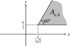
Figure 1: Integration area for the definition of the function $\mathcal{F}(a,b)$.

The results are collected in Table 1. These results obtained for Miller-Abrahams hopping rates, Eq. (55) look rather complicated for analytical estimates. Below in Sec. V we use these expressions from Table 1 for numerical calculations and present the results for the Miller-Abrahams hopping rates, Eq. (55). Here we will proceed with analytical calculations based on slightly modified expressions for the hopping rates, which allow straightforward analytical estimates. We suggest to use, instead of Eq. (55), the following “modified Miller-Abrahams rates” :

$$\Gamma_{i,i\pm 1}=\Gamma_{0}\left[1+\exp\left(\frac{\Delta\varepsilon_{i,i\pm 1}}{kT}\right)\right]^{-1},$$ (74)

where the constant $\Gamma_{0}$ will be set equal to unity for the sake of simplicity. The difference between Eq. (55) and Eq. (74) becomes negligible when $|\Delta\varepsilon_{i,i\pm 1}|\gg kT$. Therefore, for $\sigma\gg kT$ we expect a good agreement between results obtained with these two kinds of hopping rates.

Results for the “modified Miller-Abrahams rates” are also shown in Table 1. Substituting them into Eqs. (70), (IV.0.4), one can get the explicit expressions for the drift velocity and the diffusion coefficient:

$$|v|=d\,\frac{B-1}{2A+B-1},$$ (75)

$$D=d^{2}\,\frac{4A^{4}(B-1)^{2}+16A^{3}(B-1)+16A^{2}+2A(3B+1)(B^{2}-1)+(B-1)^{3}(B+1)}{2(B+1)(2A+B-1)^{3}},$$ (76)

where $A=\exp(\sigma^{2}/(kT)^{2})$, $B=\exp(|eF|d/kT)$.

Now we will consider the mobility $\mu(F)=v(F)/F$ and the diffusion coefficient $D(F)$ in the limit of small field. We restrict ourselves to the case of modified Miller-Abrahams rates. For $F=0$, one can obtain from Eqs. (75) and (76):

$$D(0)=\mu(0)\,\frac{kT}{e}=\frac{d^{2}}{2}\exp(-(\sigma/kT)^{2}).$$ (77)

For small temperatures, $kT\ll\sigma$, the mobility and the diffusion coefficient can be approximated by simple expressions:

$$\mu(F)\approx\frac{ed^{2}}{2AkT}+\frac{|Fe|ed^{3}}{4A(kT)^{2}}+\frac{F^{2}e^{3}d^{4}}{12A(kT)^{3}}\,,$$ (78)

$$D(F)\approx\frac{d^{2}}{2A}+\frac{|Fe|d^{3}}{2kT}+\frac{F^{2}e^{2}d^{4}A}{8(kT)^{2}}+\frac{|Fe|^{3}d^{5}A}{16(kT)^{3}}\,.$$ (79)

These approximations are valid for sufficiently small fields, $|eFd|<kT$.

From the latter approximated expressions it is obvious that there is a cusp at $F=0$ for both $\mu(F)$ and $D(F)$. The dependence $D(F)$ demonstrates a linear behavior for very small fields $(|eFd|\ll kT/A)$, when the first two terms in Eq. (79) are dominating, and a parabolic behavior for intermediate fields $(kT/A\ll|eFd|\ll kT)$, when the third term is dominating.

V Numerical results

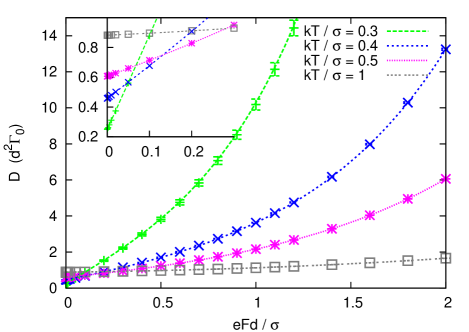
Figure 2: $D(F)$ in the RBM for different temperatures $T$. The curves show the analytical solution Eq. (III), while the symbols show numerical results (Eq. V) for chains with $N=10^{7}$ sites. The inset shows the low-field behavior.

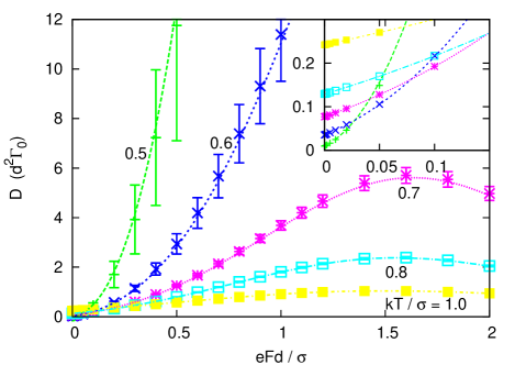
Figure 3: $D(F)$ in the REM for different temperatures $T$. The curves show the analytical solution (Eq. (IV.0.4) with $m_{1}\dots m_{11}$ from the MA column in Table 1). The symbols show numerical results (Eq. V) for chains with $N=10^{8}$ sites. The inset shows the low-field behavior.

In order to verify the analytical results obtained above, we perform numerical calculations for a one-dimensional chain of $N$ hopping sites using the equations that give the drift velocity $v$ and the diffusion coefficient $D$ as a function of all the hopping rates $\Gamma_{i\pm 1,i}$ in the chain Derrida (1983):

$$D={} \frac{1}{(\sum_{n=1}^{N}r_{n})^{2}}\Bigg{(}v\sum_{n=1}^{N}u_{n}\sum_{i=1}^{N}ir_{n+i}+$$

$$N\sum_{n=1}^{N}\Gamma_{n,n+1}\ u_{n}r_{n}\Bigg{)}\ -\ v\frac{N+2}{2},$$ (80)

$$v=\frac{N}{\sum_{n=1}^{N}r_{n}}\left[1-\prod_{n=1}^{N}\left(\frac{\Gamma_{n+1,n}}{\Gamma_{n,n+1}}\right)\right],$$ (81)

$$r_{n}=\frac{1}{\Gamma_{n,n+1}}\left[1+\sum_{i=1}^{N-1}\prod_{j=1}^{i}\left(\frac{\Gamma_{n+j,n+j-1}}{\Gamma_{n+j,n+j+1}}\right)\right],$$ (82)

$$u_{n}=\frac{1}{\Gamma_{n,n+1}}\left[1+\sum_{i=1}^{N-1}\prod_{j=1}^{i}\left(\frac{\Gamma_{n-j+1,n-j}}{\Gamma_{n-j,n-j+1}}\right)\right].$$ (83)

In this section, we follow Ref. Derrida, 1983 and set the distance $d$ between sites equal to unity for the sake of simplicity.

For both the RBM and the REM, the diffusion coefficient was obtained for different temperatures and fields, by generating several chains with random jump rates (according to the respective model), evaluating Eq. (V) for each chain and averaging the results. Long chains ($10^{7}$ and $10^{8}$ sites) were needed to obtain a good agreement between different realizations of the chains.

For chains of this length, a direct evaluation of Eqs. (V)–(83) is not practical. Below, the equations are rewritten in a form that can be evaluated in $O(N)$ steps, using recursion relations. Define

$$g_{n}=\frac{\Gamma_{n,n-1}}{\Gamma_{n,n+1}}\quad\text{ and }\quad h_{n}=\frac{\Gamma_{n+1,n}}{\Gamma_{n,n+1}},$$ (84)

and further

$$G_{n} =1+\sum_{i=1}^{N-1}\prod_{j=1}^{i}g_{n+j}$$ (85)

$$H_{n} =1+\sum_{i=1}^{N-1}\prod_{j=1}^{i}h_{n-j},$$ (86)

so that $r_{n}=G_{n}\ /\ \Gamma_{n,n+1}$ and $u_{n}=H_{n}\ /\ \Gamma_{n,n+1}$. All $G_{n}$ and $H_{n}$, and thus $r_{n}$ and $u_{n}$ can now be calculated efficiently from

$$G_{n-1}=g_{n}G_{n}-G+1,$$ (87)

$$H_{n+1}=h_{n}H_{n}-H+1$$ (88)

where $G=H=g_{1}g_{2}\ldots g_{N}=h_{1}h_{2}\ldots h_{N}$. For the first term in the brackets in Eq. (V), define $S_{n}=\sum_{i=1}^{N}ir_{n+i}$ and $S=\sum_{i=1}^{N}r_{n}$. Now

$$S_{n+1}=S_{n}-S+Nr_{n+1}.$$ (89)

These relations are numerically stable if $G<1$, which is satisfied if the average drift is to the right (towards larger site indices). The diffusion coefficient is now given by

$$D=\frac{1}{S^{2}}\left(v\sum^{N}_{n=1}\frac{H_{n}S_{n}}{\Gamma_{n,n+1}}+N\sum^{N}_{n=1}\frac{G_{n}H_{n}}{\Gamma_{n,n+1}}\right)-v\frac{N+2}{2}.$$ (90)

It seems tempting to write Eq. (87) in the form

$$G_{n}=(G_{n-1}+G-1)/g_{n},$$

so that all equations could be evaluated starting from $n=1$, but this form is too susceptible to numerical errors to be usable in practice. Thus one has to evaluate all $G_{n}$ with Eq. (87) starting from $G_{N}$ and store them in a table. $S_{n}$ and $H_{n}$ do not need to be stored, since they can be evaluated while performing the sum in Eq. (90), starting from $n=1$.

With this method of evaluation, numerical results for the diffusion coefficient were obtained. The results are shown in Fig. 2 for the RBM, together with the analytical results, and in Fig. 3 for the REM. For both models the diffusion coefficient is linear in the electric field (at low fields), see the insets in each figure.

VI Discussion and conclusions

Figures 2 and 3 demonstrate a full agreement between analytical results, Eqs. (III) and (IV.0.4), and numerical ones based on Eq. (V). This result can be considered as evidence that the two definitions of the diffusion coefficient $D$, Eq. (8) and Eq. (9), give the same quantity for hopping in one-dimensional disordered systems. The former definition expresses $D$ via the variance of particle displacement during a random walk, while the latter one defines $D$ as a ratio between the particle flow and the gradient of macroscopic concentration of particles. Although it seems to be obvious from a physical point of view that both definitions should give the same result, no formal proof has yet been known.

Computer simulations evidence that at low temperatures the diffusion constant experiences significant fluctuations from one realization to another, even for systems containing millions of localized states. The reason of such a large fluctuations in 1D hopping is essentially the same as in 3D hopping—it is the sensitivity of the diffusion coefficient to the very rare sites with low energies. We will discuss this phenomenon in detail in the following paper.Nenashev et al. (2009) We also note that sample-to-sample fluctuations of mobility for all parameters presented in Figures 2 and 3 are negligible.

The most striking property of the 1D diffusion is its linear dependence on electric field:

$$D(F)=D(0)+\alpha|F|+O(F^{2})\,,$$ (91)

where $\alpha\neq 0$. It means that the diffusion coefficient is a non-analytic function of electric field. From general physical arguments one can hardly expect such a behavior. Instead, one can expect that, as $D(F)$ is an even function, it can be expanded in a Taylor series with respect to $F^{2}$:

$$D(F)=D(0)+\beta F^{2}+O(F^{4})\,.$$ (92)

The physical reason of this non-analyticity is still unclear. As first steps to acquire an understanding of this phenomenon, we will try (i) to provide a mathematical explanation of it and (ii) to find out which systems demonstrate the linear field dependence of the diffusion coefficient and which systems lack this behavior.

From the mathematical point of view, the possibility for a non-analytic dependence $D(F)$ can be seen from expressions (30) and (39) for the coefficients $a_{i}$ and $b_{i}$ as functions of $B\equiv\exp(eFd/kT)$. These expressions are series that converge at $B>1$ and diverge at $B\leq 1$. For $B<1$ (i. e. for negative $eF$) one can obtain converging series, applying a “mirror reflection” transformation ($i+k\rightarrow i-k$, $B\rightarrow B^{-1}$) to Eqs. (30) and (39). Therefore $a_{i}$ and $b_{i}$ are defined by different series expansions for positive and negative values of the field. Moreover, at $eF>0$ the values $a_{i}$ and $b_{i}$ depend on quantities related to sites $i$, $i+1$, $i+2$, … (for example, on $\Gamma_{i+1,i+2}$, $\varepsilon_{i+1}$, etc.); on the contrary, for $eF<0$ these coefficients $a_{i}$ and $b_{i}$ depend on a different set of sites: $i$, $i-1$, $i-2$, … So, it is obvious that, in a disordered system, the function $a_{i}(F)$ for negative $F$ cannot be obtained by analytic continuation of this function for positive $F$, and vice versa. The same is true for $b_{i}(F)$. Keeping in mind that the mobility $\mu\equiv v/F$ and the diffusion coefficient $D$ depend on $a$’s and $b$’s via Eq. (27), one can conclude that negative-field parts of the functions $\mu(F)$, $D(F)$ may not be analytic continuations of their positive-field parts. Consequently, a non-analyticity of $\mu(F)$ and $D(F)$ at $F=0$ is possible.

It is evident from Figs. 2 and 3 and from Eqs. (III) and (79) that both the RBM and the REM demonstrate a linear low-field behavior of $D(F)$, according to Eq. (91). Moreover, Eq. (78) shows that the mobility $\mu(F)$ in the REM also contains a linear contribution with respect to $F$, while in the RBM the mobility is a smooth function of $F$, see Eq. (53).

Parris et al.Parris et al. (1997a, b) considered a model of a 1D continuous medium with smooth disorder potential, and obtained analytical expressions for $\mu(F)$ and $D(F)$. Although the low-field behavior of the mobility and of the diffusion coefficient were not discussed in detail,Parris et al. (1997a, b) one can learn from equations (25) and (69) of Ref. Parris et al., 1997b that this behavior is qualitatively the same as in our REM. The method of Refs. Parris et al., 1997a, b is, however, not directly applicable to the Gaussian disorder model considered here. Therefore a separate derivation was necessary.

One-dimensional transport with Gaussian density of states (DOS) has another peculiarity—namely, there are sites with arbitrarily high energies, which represent barriers for transport. Despite the fact that such barriers are very rare, their influence on the transport properties should be noticeable (unlike in the 2D and 3D cases, where a carrier can easily pass around these hard places). One can argue that this peculiarity might be responsible for the unusual non-analytical behavior of $\mu(F)$ and $D(F)$. In order to check this assumption, we consider a 1D system with a discrete DOS $g(\varepsilon)$ allowing only two values of energy ($\varepsilon=-\sigma$ and $\varepsilon=\sigma$):

$$g(\varepsilon)=\frac{1}{2}\delta(\varepsilon+\sigma)+\frac{1}{2}\delta(\varepsilon-\sigma).$$ (93)

It is obvious that there are no high barriers in this system. Using our general expressions (50), (51), (70), and (IV.0.4), we have calculated the dependencies $\mu(F)$ and $D(F)$ for this DOS for both RBM and REM. The results demonstrate qualitatively the same low-field behavior as in the case of Gaussian DOS. Therefore the property of the non-analyticity of $\mu$ and $D$ cannot be attributed just to the presence of infinitely high barriers provided by the corresponding DOS.

We have also checked whether this non-analyticity is related to the assumption of the nearest-neighbor hopping. We have considered the same random-energy model as discussed in Sec. IV, except that we allow transitions to distant states. The dependence of transition rates $\Gamma_{ij}$ on distances $r_{ij}$ between the sites is governed by the Miller-Abrahams expression (3). The mobility and diffusion coefficient as functions of electric field were calculated by a Monte-Carlo algorithm described in the following paper.Nenashev et al. (2009) Again, the results have shown linear low-field dependencies $\mu(F)$ and $D(F)$.

Therefore one can conclude that the linear behavior of the diffusion coefficient, Eq. (91), is a robust property of 1D disordered systems.

On the contrary, at higher dimensions there are no evidences of a linear field dependence of the diffusion coefficient. Both our Monte-Carlo simulations (see the following paper, Ref. Nenashev et al., 2009) and previous studiesPautmeier et al. (1991) clearly demonstrate a parabolic field dependence, Eq. (92), for 2D and 3D systems with Gaussian disorder. It is worth to note that a smooth dependence $D(F)$ should be obtained also in 1D systems without disorder—namely, in systems with periodically repeated site energies (and barrier heights). Indeed, such a system is equivalent to a finite chain (with periodical boundary conditions) considered by Derrida.Derrida (1983) One can therefore use Derrida’s formula for $D$, Eq. (V). This formula, in the case of finite chain length $N$, is an analytic function of the transition rates $\Gamma_{ij}$, and consequently of the electric field. Our numerical studies also confirm that for small $N$ there is a region of parabolic dependence $D(F)$ around $F=0$. Thus, disorder is important for the non-analytic behavior of $D(F)$.

Finally, we will discuss the applicability of Einstein’s relation (1) for finite electric fields. Our analytical results, Eqs. (53), (III), (78), and (79) show that Einstein’s relation is violated at any non-zero field $F$ both in RBM and REM, and that the deviation from Eq. (1) is proportional to $|F|$. One should note that this phenomenon is related to the discrete nature of the systems, in which charge transport is dominated by hopping processes. For the opposite case of a continuous-medium model, the diffusion coefficient is known to obey a generalized version of the Einstein relation:Parris et al. (1997a, b)

$$D(F)=\frac{kT}{e}\,\frac{dv}{dF}\,,$$ (94)

where $v(F)$ is the drift velocity. Our expressions for both RBM and REM, however, demonstrate that Eq. (94) is also violated in the general case, and the deviation is also proportional to $|F|$. We argue that, generally, there are no exact connections between $D(F)$ and $\mu(F)$ at $F\neq 0$. Indeed, let us consider the REM. There are eleven quantities $m_{1}\ldots m_{11}$ (see Sec. IV) dependent on statistics of the energy levels and on the electric field. The mobility depends on three of them ($m_{1},m_{3},m_{4}$), according to Eq. (70); the diffusion coefficient depends on all eleven quantities, see Eq. (IV.0.4). For an arbitrary density of states, all the eleven quantities are independent of each other and cannot be reduced to each other. Consequently, there is no general way to reduce the diffusion coefficient to the mobility at non-zero electric field.

In conclusion, we have examined analytically and numerically two models of one-dimensional hopping transport—the random-barrier (RBM) and the random-energy model (REM). Exact analytical solutions of field-dependent diffusion coefficient have been obtained for both models in the case of nearest-neighbor hopping. We have demonstrated that the non-analytic field dependence (91) of the diffusion coefficient, as well as the violation of the Einstein relation for any nonzero electric field, are inherent properties of hopping transport in one-dimensional disordered systems.