A detailed study of the main sequence of the Globular Cluster NGC 6397:

Abstract

Aims. If NGC 6397 contains a large fraction of “second generation” stars ($>$70% according to recent analysis), the helium abundance of its stars might also be affected, show some star-to-star variation, and be larger than the standard Big Bang abundance Y$\sim$0.24. Can we derive constraints on this issue from the analysis of the main sequence width and from its luminosity function?

Methods. We build up new models for the turnoff masses and the main sequence down to the hydrogen burning minimum mass, adopting two versions of an updated equation of state (EOS) including the OPAL EOS. Models consider different initial helium and CNO abundances to cover the range of possible variations between the first and second generation stars. We compare the models with the observational main sequence. We also make simulations of the theoretical luminosity functions, for different choices of the mass function and of the mixture of first and second generation stars, and compare them with the observed luminosity function, by means of the Kolmogorov Smirnov –KS– test.

Results. The study of the widht of the main sequence at different interval of magnitude is consistent with the hypothesis that both generations are present in the cluster. If the CNO increase suggested by spectroscopic observation is taken into account the small helium spread of the main sequence in NGC 6397 implies a substantial helium uniformity ($\Delta$Y$\sim$0.02) between first and second generation stars. The possible spread in helium doubles if an even larger increase of CNO is considered. The luminosity function is in any case well consistent with the observed data.

1 Introduction

Our views about Globular Clusters (GCs) are dramatically changing in these latter years, thanks to precise photometric investigations, that revealed the presence of multiple main sequences or subgiant branches (e.g. Piotto et al., 2007; Milone et al., 2008), and the increasing amount of new spectroscopic data on GC stars. These data, in particular the spectra for about 2000 stars in 19 GCs recently obtained by the multiobject spectrograph FLAMES@VLT (Carretta et al., 2009a, b) have shown how the “chemical anomalies” among GC stars are indeed ubiquitous in all clusters, and concern a large fraction (from 50 to 80%) of stars. The peculiar chemical abundances take the form of anticorrelations between O and Na, Al and Mg, and are present in stars of various evolutionary phases (both unevolved main sequence and evolved red giant branch stars) (Gratton et al., 2001; Ramírez & Cohen, 2002; Carretta et al., 2004), supporting the idea that they are not due to an “in situ” deep mixing in the stars, but have been imprinted in the gas from which they formed, that was polluted by the winds lost by a previous first generation (FG) of stars: according to this hypothesis, we are now seeing a second generation (SG) of stars mixed to the FG. It is not definitely settled what kind of stars produced this material, that must have been processed by the hot CNO cycle and other proton capture reactions on light nuclei. The two most popular candidates are massive asymptotic giant branch (AGB) stars (e.g. Ventura et al., 2001), and possibly, for the extreme anomalies, super–AGBs (Pumo et al., 2008), or massive stars, either fastly rotating (e.g. Decressin et al., 2007), or in binaries undergoing non conservative evolution (de Mink et al., 2009).
Carretta et al. (2009a) examine the famous Na–O anticorrelation and tentatively divide the stars of each cluster in three groups: the “primordial” stars, those having abundances of O and Na similar to those found in the halo stars; the “intermediate” stars, having high Na and somewhat depleted O; the “extreme” stars, having high Na and strongly depleted O. While only a few, very massive, clusters contain stars with extreme anomalies, all clusters show a population with “intermediate” chemistry. The problem of GC formation and early evolution is very complex, but it is easy to accept that a cluster contains two or multiple populations, if it shows both chemical peculiarities, as discussed above, and photometric peculiarities: the GC NGC 2808 is a prototype of this class, as it shows three populations both in the main sequence (Piotto et al., 2007) and in its horizontal branch (HB) extended morphology (D’Antona & Caloi, 2004), and it is possible to reproduce these three populations by assuming that they differ in helium content (e.g. D’Antona & Caloi, 2008); in addition, this cluster shows the Na–O anticorrelation in one of its most extreme forms, with stars reaching very low oxygen abundances. Carretta et al. (2006) even find a possible indirect hint of helium enhancement in the subgroup of oxygen–poor red giants that they examine. As theory expects that some helium enrichment accompanies the hot–CNO nucleosynthesis in both the proposed models (massive AGBs or massive stars), NGC 2808 represents in many respects, the most classic example of well understood multiple populations in GCs.

There are other cases, however, in which the presence of subpopulations is not as well clear, and, in particular, it is not clear whether the abundance anomalies (in some cases less prominent, but always present, according to Carretta et al., 2009a) are always accompanied by helium enrichment, and how large this enrichment is. In particular, the cluster NGC 6397 has always been considered the perfect example of a “simple stellar population” (SSP) due to the “tightness” of its HR diagram, including a very compact blue HB. In recent years, spectacular data for the low main sequence of NGC 6397 have become available. By using the technique of proper motion cleaning, Richer et al. (2006) obtained a very tight main sequence and a very clean luminosity function down to the hydrogen burning minimum mass (HBMM) (Richer et al., 2008). We decided to use these data to quantify at what level we can accomodate helium variations in this cluster (and the possible, associated, CNO variations), by investigating whether the main sequence width and its luminosity function are compatible with a helium spread and/or with a non–standard helium content. At the same time, we take the occasion of this comparison to compute and test new stellar models for the low main sequence. In these models, we employ and compare new equations of state (EOS) today available, and we test the available color-T_eff transformations.
The outline of the paper is the following. In Section 2 we describe in some detail the spectroscopic results concerning the cluster, and what we expect concerning the multiple populations it should hide, and what are plausible helium and C+N+O variations expected. We then summarize the photometric data by Richer et al. (2008). After having summarized the literature concerning the low mass main sequence models, in Section 3 and 4 we describe our code and the results of the computation of solar scaled models; in Section 5 we present $\alpha$-enhanced models computed for the comparison with the data for the Globular Cluster NGC 6397. Both the comparison of the CMD and the luminosity function with theory are discussed in detail in Section 6 also in the hypothesis of multiple populations with different helium, and possibly also C+N+O, content. In Section 7 we summarize our results and conclusions.

2 The case of NGC 6397: apparently, a simple stellar population

Carretta et al. (2009a) find that at least 70% of stars in the cluster NGC 6397 are “intermediate” according to their definition, although photometric studies show that all the evolutionary sequences in this cluster look like those of a prototype SSP: the main sequence is very tight (King et al., 1998; Richer et al., 2006), and the horizontal branch (HB) lacks the extreme HB and blue hook stars that are now regarded as the proof of the presence of a very helium enriched population (D’Antona et al., 2002; D’Antona & Caloi, 2004). The chemical anomalies of Carretta et al. (2009a) analysis, however, do not come as a full surprise, as already many hints were available in the recent literature about the dubious simplicity of this cluster. First of all, already Bonifacio et al. (2002) had noticed the presence of Nitrogen rich stars that have a normal Lithium content (see also Pasquini et al., 2008), and Carretta et al. (2005) find that only three subgiants out of 14 stars are nitrogen normal. These features lead us to suspect that the material from which these stars formed is CNO processed, as expected in the stars with low oxygen and high sodium. The possible helium enhancement is certainly not extreme, as, for instance, are small lithium variation among the turnoff stars (Lind et al., 2009; Korn et al., 2007; Pasquini et al., 2008). In the massive AGB model for the formation of the second generation, the lithium content of the AGB ejecta is not extremely depleted as in the other models, but it is difficult to believe in a cosmic conspiracy producing exactly the same lithium of the FG, unless the AGB matter is very diluted with FG gas, so that both lithium and helium do not differ too much in the two generations.
A different, mostly theoretical, approach, led Caloi & D’Antona (2005) and then D’Antona & Caloi (2008) to provocatively propose that all the stars in the clusters having entirely blue HBs are composed by SG stars. This idea is at the basis of a possible explanation of the peculiar difference between the GCs M 3 and M 13. The cluster M 3 has a complex HB, including many stars redder than the RR Lyrae (a red clump), RR Lyrae stars, and a well populated blue side, while M 13, having the same metallicity, has an only–blue HB. This difference, that has been generally attributed to different age (Johnson & Bolte, 1998; Rey et al., 2001) or to different mass loss along the red giant branch (Lee et al., 1994; Catelan et al., 1998) (the famous second parameter problem) may also be interpreted by assuming that M 13 is totally deprived of its FG, and the SG has a minimum helium abundance in mass fraction Y$\sim$0.28. In M 13, whose HB shows a prominent blue tail, simulations of the HB stellar distribution show that there must also be a small fraction of stars with helium Y$\sim$0.38 (D’Antona & Caloi, 2008). Is it possible that a GC is composed only of SG stars? This could indeed happen, as shown in some hydrodynamic plus N–body simulations of the SG formation and of the cluster first phases of dynamical evolution presented by D’Ercole et al. (2008). They find that the dynamical evolution of the cluster may be characterized by expansion of the FG star system due to the SNII mass loss preferentially occurring in the cluster central regions, while the SG is still forming in the core. Depending on the initial conditions, in some cases, the ratio of SG to FG stars may even reach a factor 6 or more. While this kind of modelling depends on the input parameters, and does not imply that this really occurred in nature, NGC 6397, having a short blue HB, and a tight main sequence (MS) and red giant branch (RGB), could indeed be made by a homogeneous set of SG stars, corresponding to a unique value of Y, just a bitter larger than the Big Bang abundance (Y$\sim$0.26-0.28). This speculation would help to understand why the nitrogen abundance in most of the NGC 6397 stars is quite large. The possibility that all the stars in this cluster have a homogeneous, but larger than standard, helium abundance could be falsified by looking at the main sequence width, that depends on the combination of the photometric errors with the possible star to star differences in helium.
Apart from this extreme and provocative suggestion, very recently Carretta et al. (2009a) show that only up to $\sim$30% of stars should belong to the primordial population (the FG), in the assumption that all the stars within three sigma from the lowest sodium abundance measured in a cluster are “primordial”. So, at present, the most reasonable assumption is that NGC 6397 has at least 70$\%$ of SG.
Given the sodium and oxygen abundances of the anomalous cluster stars, do we expect that they have an enhanced helium content? In the hypothesis that the SG is born from matter mixed with the hot–CNO processed ejecta of massive AGBs, we can look at the results by Ventura & D’Antona (2009). They interpret the anomalous Na–O abundances in NGC 6397 as a result of mixing between 50% of pristine gas with 50% of gas ejected by the 5M_⊙ AGBs. Looking at Table 2 of their paper, the helium abundance in the 5M_⊙ ejecta for Z=0.0006 is Y=0.329. A dilution by 50% with matter having primordial Y=0.24 provides indeed Y=0.285. If we take these results at face value, also the total CNO content of the SG stars is larger than that of the FG stars. The 5M_⊙ AGB evolution provides a CNO enhancement by a factor $\sim$3, so we must consider also increased CNO (and total metallicity) by a factor 1.5, when we compute the higher helium models. Of course, the computed AGB models do not give a mandatory prescription of what really happens in the cluster, so that we will also consider normal CNO models and models with even larger CNO in order to include all possible cases. Helium abundances equal or larger than the standard one will be considered, up to Y=0.28, to understand whether the hypothesis that at least $\sim 70$% of stars in NGC 6397 have an helium abundance larger than the Big Bang abundance is consistent with the photometric data.

2.1 The observational color-magnitude diagram of Globular Cluster NGC 6397

The first HST observations of the low MS of NGC 6397 date back to Paresce, De Marchi & Romaniello (1995). Afterwards, King et al. (1998) have observed NGC 6397 with WFPC2@HST finding that the luminosity function has a rapid decline at low mass end. Recently, the deepest observations by Richer et al. (2006, 2008) refined the data. They observed an outer region of NGC 6397 with ACS@HST using the photometric filters F814W and F606W. The high sensitivity of the camera, the large number of orbits obtained (=126) and the vicinity of the cluster (it is the second closest globular cluster, after M4) made it possible to reach the deepest intrinsic luminosities for a globular cluster achieved until today, and what appears as the termination of the MS. The field observed overlaps that of archival WFPC2 data from 1994 and 1997, which were used for the proper-motion-cleaning of the data. This technique, applied to the deep ACS photometry, produces a very narrow MS till its end. These observations are a good basis to test the physics of low mass stars and the possible role of the helium abundance. Richer et al. (2008) analyzed the color-magnitude diagram (CMD) diagram using the results of models computed with Dartmouth Stellar Evolution Program (DSEP) (Dotter et al., 2007). Their main results are that:

• the MS appears to terminate close to the CMD location of the HBMM predicted by models. The authors state that they would have found fainter MS stars in the cluster, if there had been any;

• the MS fitting technique provides a good agreement down to F814W=22.5 mag; below this, down to $\sim$24 mag, the isochrone is either too blue or too low in luminosity. The authors underline that this is likely due to low mass models being less luminous at a given mass than real stars;

• exploring the MS luminosity function, they find that a power law for the mass function MF well reproduces the distribution in luminosity of the observed stars, while a more top–heavy MF is necessary to fit the data in the cluster core that they have also available. However, theory predicts more stars than observed at the lowest MS luminosities, as also previously found by Montalban, D’Antona & Mazzitelli (2000) using data by King et al. (1998)

3 The low mass main sequence models:Input Physics of the models

The computation of very low mass stellar models requires an accurate knowledge of the EOS for partially ionized gas at densities where the ideal gas EOS approximations breaks down dramatically, especially close to the pressure ionization region (Fontaine et al., 1977; Magni & Mazzitelli, 1979; Saumon, Chabrier & van Horn, 1995). The general properties of very low masses have been described in many works (for example see the reviews by Chabrier & Baraffe, 1997; Alexander et al., 1997; Cassisi et al., 2000); for the population II low masses, after the work by D’Antona (1987), based on grey atmosphere boundary conditions and on the EOS by Magni & Mazzitelli (1979), Baraffe et al. (1997) presented models based on the Saumon, Chabrier & van Horn (1995) EOS and on the NextGen non-grey atmosphere models later on published by Hauschildt, Allard & Baron (1999). They showed that this latter improvement was essential to reproduce the colors of the low mass main sequence. Montalban, D’Antona & Mazzitelli (2000), reexamining the problem of the EOS, cautioned about the use of the Additive Volume interpolation needed to obtain the thermodynamic quantities for intermediate compositions from the pure hydrogen and pure helium tables available in the Saumon, Chabrier & van Horn (1995) EOS. In recent years, two new EOS have become available: the FreeEOS by Irwin (2004) and the OPAL EOS, namely the EOS provided by the Livermore group as a byproduct of the opacity computation (Rogers et al., 1996). Both EOS however do not cover the pressure ionization region, for which the best approach remains that by Saumon, Chabrier & van Horn (1995).The FreeEOS has been recently employed by Dotter et al. (2007) and applied to the fit of the main sequence of NGC 6397. The OPAL EOS has not yet been used to approach the construction of low mass models, so we decided to adopt it in two different ways in our new models, as described in Sect. 4.
We use the ATON code for stellar evolution; a detailed description can be found in Ventura, D’Antona & Mazzitelli (2007); in the following we remember the main updated inputs that are important for the treatment of low mass stars.

3.1 Opacities and nuclear reaction

The program includes the opacities by Ferguson et al. (2005) for the external region of the star (T$\leq$15000 K) and the latest version (2005) of OPAL opacities for higher temperatures (Iglesias & Rogers, 1996). For fully convective low mass stars (below $\sim$0.35M_⊙), the uncertainties on radiative opacities have negligible influence on the models, while for larger masses an error in opacity by $\sim$20$\%$ may cause an error up to $\sim$1$\%$ in the determination of radii (Dotter, 2007). Electron conduction opacities were taken from the WEB site of Potekhin (2006) and correspond to the Potekhin et al. (1999) treatment, corrected following the improvement of the treatment of the e-e scattering contribution described in Cassisi et al. (2007).
Although not necessary in this computation, the nuclear network includes 30 chemical elements, all main reactions of p-p, CNO, Ne-Na and Mg-Al chains and the $\alpha$ capture of all nuclei up ²⁶Mg. The relevant cross section are from the NACRE compilation (Angulo et al., 1999).

3.2 Equation of state: OPAL vs Saumon, Chabrier & van Horn (1995)

Figure 1: We show the region of the Log($\rho$)-Log(T) plane (density $\rho$ in g cm^-3 and temperature T in K) where OPAL (solid box) and SCH (dashed box) EOS are available. The structure profile of two stars with Age=10 Gyr, Z=0.0006 and with M=0.6 M_⊙ and 0.1 M_⊙ are also shown. The 0.6M_⊙ is in the region of overlapping of the two EOS, while 0.1M_⊙ is exactly at the border between the two EOS.

Figure 2: Adiabatic gradient ($\nabla_{\rm ad}$; dash-dotted and dotted curves; right y-axis) and molecular weight ($\mu$, solid and dashed curves; left y-axis) as a function of pressure P (cgs units) for the structure with M=0.3 M_⊙, Z=0.0006, Y=0.24 and Age=10 Gyr. The solid and dash dotted curves correspond to EOS+OPAL while dashed and dotted curves are calculated with EOS+SCH (see text).

As remarked previously, non-ideal effects become increasingly important for masses M$\;\buildrel<\over{\sim}\;$ 0.8M_⊙.
ATON uses 18 tables of EOS in the (gas)pressure-temperature plane corresponding to three different metallicities, Z=0, 0.02 and 0.04, and six hydrogen mass fractions X, ranging from 0 to 1-Z; the thermodynamic quantities, i.e. density, adiabatic gradient, specific heat at constant pressure C_p, the C_p/C_v ratio, and the three exponents $\Gamma_{1}$, $\Gamma_{2}$ and $\Gamma_{3}$ are obtained via 4 cubic unidimensional splines on X, Z, pressure and temperature.
These 18 tables are built up in three steps. First, the thermodynamic quantities are computed according to the formulation by Stolzmann & Blöcker (2000), which is the most modern and updated description available for ionized gas, including both classic and relativistic degeneracy, coulombian effects and exchange interaction. The tables are then partially overwritten by the OPAL EOS in the whole domain where this is available (Rogers et al., 1996, see OPAL WEB page, last update in February 2006). Finally in the very low-temperature regime, where OPAL EOS is not available (see Fig. 1) the tables are overwritten by the Saumon, Chabrier & van Horn (1995) EOS, which has the advantage of employing an adequate physical model for the pressure ionization. The Saumon et al. EOS is only given for pure hydrogen and pure helium mixtures; the presence of metals is thus simulated by adding helium, and the different H-He mixtures must be interpolated through the Additive Volume law.
We call “EOS+OPAL” these tables, that represent the standard in our computations. To investigate how the results depend on the chosen EOS, we built additional tables (EOS+SCH) using the EOS by Saumon, Chabrier & van Horn (1995, SCH) in the whole region of the P-$\rho$ plane for which it is available. This is an interesting test, because the structure of the majority of stars discussed here are contained in the region of plane LogT-Log$\rho$ where both EOS are available (see Fig. 1).
In Fig. 2 we show the differences in the molecular weight ($\mu$) and adiabatic gradient $\nabla_{\rm ad}$=d$\log$P/d$\log$T along the structure of two main sequence models of M=0.3M_⊙, Z=0.0006 at the age of 10Gyr, computed with the two different EOS. The differences are more evident in the zone of partially ionization where physical differences of the two treatments (different $\mu$) affect $\nabla_{\rm ad}$. In the EOS+SCH models, the regions in which $\nabla_{\rm ad}$ is lower prevail, and the global effect is to produce T_eff larger by about 100 K, practically at the same luminosity, since the inner structure does not change significantly with the EOS.
The results for different masses are shown in Fig.3, reporting the HR location of the models at 10Gyr. The differences are small for M$\geq$0.5M_⊙, where the regions of partial ionization do not dominate, and vanish at the lowest masses, because only the EOS+SCH is available for the physical conditions of their interiors.
Based on these results, we may conclude that use of both EOS leads to models with compatible effective temperatures and luminosities. In Fig.3, for the available masses, we report the location of the models of same chemistry computed by Dotter et al. (2007) with the Dartmouth Stellar Evolution Program (DSEP), using the FreeEOS by Irwin (2004) and otherwise a very similar input physics (L and T_eff’s are taken from their WEB page); for the same masses also the models by Baraffe et al. (1997) are shown. Note that these latter models do not differ significantly from ours, both in L and T_eff, while the models calculated with DSEP at the lowest masses differ, especially in T_eff, up to $\sim$300 K at 0.15M_⊙. This effect can be possibly attributed at the different EOS, but a detailed comparison of models would be required.

Figure 3: HR diagram location at 10 Gyr for models with Z=0.0006, the labelled masses and calculated with different EOS tables. Models from the Dartmouth Stellar Evolution Database (full dots) and from Baraffe et al. (1997) (asterisks), with same metallicity of ours, are also shown for comparison.

3.3 Convection

The ATON code allows us to model turbulent convection by adopting the traditional Mixing Lenght Theory (MLT, Bohm-Vitense, 1958) or the “Full Spectrum of Turbulence” (FST) model (Canuto & Mazzitelli, 1991; Canuto, Goldman & Mazzitelli, 1996) which takes into account the full eddies energy distribution (see Canuto e Mazzitelli, 1991 for a detailed description of the physical differences between the two models).
While for very low mass stars the description of convection has no influence on the atmospheric structure, this does not hold for those masses in which convection has a substantial degree of overadiabaticity, especially for the stars at the turnoff of GCs. For these models a homogeneous modelling of convection in the atmosphere and the interior is highly recommended. At T_eff$>$4000K, the grids of models computed by Heiter et al. (2002) by means of NEMO, a modified version of Kurucz’s code, are available. These grids are provided both with MLT model and with the FST model by Canuto, Goldman & Mazzitelli (1996). A preliminary version of these latter grids has been used by Montalbán et al. (2001) and will be used in this paper (where possible).

3.4 Atmospheric structure and boundary condition

At T_eff$\;\buildrel<\over{\sim}\;$4000K, in the outermost layers of very low mass stars, radiative absorption is dominated by molecules, and the outcoming flux is far different from the frequency-averaged distribution provided by grey models (Baraffe et al., 1997; Montalban, D’Antona & Mazzitelli, 2000). At larger T_eff, the atmospheric models become less critical, whereas the T_eff itself is heavily influenced by the treatment of overadiabatic convection. For the non-grey models that employ an MLT treatment of convection in the atmosphere with a given $\alpha_{atm}$, not only the $\alpha=l/H_{p}$ used in the interior computation ($\alpha_{in}$) affects the T_eff, but also the optical depth at which the match between the atmospheric and the interior integration is made, and the value of $\alpha_{atm}$ (Montalbán et al., 2004). Montalbán et al. (2001) have shown that use of the NEMO grids of model atmospheres (Heiter et al., 2002) computed with the FST convection may provide a good match to the interior models computed with the same convection model in the interior, independently of the matching optical depth.

For the above two reasons we use, according to the stellar mass, boundary conditions based on two different grids of non grey models of atmosphere. For M$\geq$ 0.5M_⊙ we use Heiter et al. (2002) FST grids, and FST convection also in the interior computations, whereas for M$\leq$ 0.5M_⊙ we adopt the NextGen grids by Hauschildt, Allard & Baron (1999) computed by the PHOENIX code with the MLT treatment of convection and $\alpha_{atm}=l/H_{p}=1$. The available grids extend down to T_eff =800 K for the [M/H]=–2.0 models, but just down to 2000 K for larger metallicity. For these M$\leq$ 0.5M_⊙ models, we adopt MLT convection also in the interior computation, setting $\alpha_{in}$=2.0. Since the model atmospheres are computed assuming an ideal gas and a Saha–like thermodynamics, they should not be used in the real gas domain where pressure effects are relevant, and a relatively small value of the optical depth is chosen for the match between atmosphere and interior. We use $\tau_{ph}$=3(10) for M$<$($\geq$) 0.5M_⊙. Notice that the grids of model atmospheres available are computed only for solar scaled mixtures. The lack of suitable model atmospheres for $\alpha$-enhanced populations forces us to use for the boundary atmospheric conditions a grid with larger [Fe/H], to simulate the $\alpha$–enhancement, following the procedure adopted by Baraffe et al. (1997). We use a grid for [Fe/H]=-1.7, obtained through interpolation between the grids for [Fe/H]=-2.0 and -1.5, to compute $\alpha$–enhanced models with Z=0.0002.

3.5 Transformations to observational plane

In order to compare the models to the photometric data in NGC 6397 we convert luminosity, T_eff and surface gravity into absolute magnitudes and colors in the ACS filters. The method most used is to calculate theoretical stellar spectra from atmosphere’s models and convolving these synthetic spectra with the filter transmission curves for a photometric system which defines the transmission of light through the filter as a function of wavelength. Uncertainties derive especially from the missing or incorrect absorption features and simplifying physical laws, such the assumption of LTE. On the other hand, semiempirical colors and bolometric corrections (e.g. Vandenberg & Clem, 2003) have other uncertainties, e.g. they depend on the assumed distance (Dotter et al., 2007).
For the specific case of ACS filters, we use the procedure by Bedin et al. (2005). They computed ACS color indices by using homogeneous set of ODFNEW model atmospheres and synthetic fluxes computed with Kurucz ATLAS9 code (Castelli & Kurucz, 2004). Grids of magnitudes for different values of [Fe/H], for 3500K $\leq$ T_eff $\leq$ 50000K, 0 $\leq$ logg $\leq$ 5.0 and microturbolent velocity 2.0 km/s^-1  are provided. Visual bolometric correction BC_V, visual magnitude M_V, and color indices M_V-M_ACS are given. The ACS magnitudes were computed by using the WFC/ACS transmission curves by Sirianni et al. (2005), while they adopted the V passband from Bessel (1990). Finally, they assumed that Vega ACS magnitude would be equal to 0.00 in all passbands.
The bolometric corrections by Bedin et al. (2005) for ACS filters do not extend below T_eff$=$3500K. For these low temperatures we can use the values obtained from the synthetic spectra of Hauschildt, Allard & Baron (1999). Also in this case, the transmission filters of Sirianni et al. (2005) were used, and zero points corrections to standard system are obtained from observed Vega spectra.
Obviously the availability of a unique set of colors-Teff transformations would be highly recommended; however, at least, for masses below 0.5 M_⊙, we have the advantage of using the same bolometric corrections derived from the atmospheric structures used as boundary conditions for the stellar models.
Finally we note that the two sets of correlations match very well in the main sequence, so that no discontinuity arises in our transformed isochrones.

Figure 4: Evolutionary tracks, starting from the pre-main-sequence, for three different masses with Z=0.0006 and different value of initial helium.The filled circle label the position in HR diagram of the star at Age=10Gyr. Only for the highest mass the tracks with the all three Y are shown

4 Results: solar scaled models

We computed evolutionary tracks for low mass objects (M$\leq$0.8M_⊙) from the pre main sequence to the red giant branch, or until they reach an age of 20Gyr. Results are shown here for [M/H]=–1.5 and [M/H]=–2.0, but larger metallicities ([M/H]=–1.00 and –0.50) are available upon request.
In this Section we present results for solar scaled mixtures (Grevesse & Sauval, 1999, GS1999), [$\alpha$/Fe]=0.4 models will be used in the Section 6 to compare with the data of NGC 6397. Models are extended down to the HBMM when the atmospheric boundary conditions allow it.
We computed standard evolutionary tracks with an initial helium content close to the Big Bang abundance (that is Y=0.24, Coc et al., 2004), and models with larger helium (Y=0.28, 0.32 and 0.40). From the evolutionary tracks, isochrones are derived for typical ages expected for GCs, from 10 to 14 Gyr.
Fig. 4 compares the HR diagram evolution for three different masses (M=0.70, 0.30 and 0.10 M_⊙) and different Y. Models with a larger helium abundance have larger luminosity and T_eff, due to the average larger mean molecular weight $\mu$. This effect is more evident in the stars with a radiative core (here shown is the M=0.7M_⊙) than in the totally convective stars like the 0.3M_⊙. The difference increases again in the lowest masses ($\;\buildrel<\over{\sim}\;$0.15 M_⊙), where partial degeneracy begins playing a role.

4.1 Mass-luminosity relation

Figure 5: The MLR for models at 10 Gyr having the labelled value of metallicity and different helium abundance (=0.24-open circles, =0.28-filled triangles, =0.32-filled circles, =0.40-asterisks). In each case the lower masses are the derived HBMM and reported in Table 1.

Figure 6: Comparison at very low masses between the MLR obtained using models computed with different equations of state (see text).

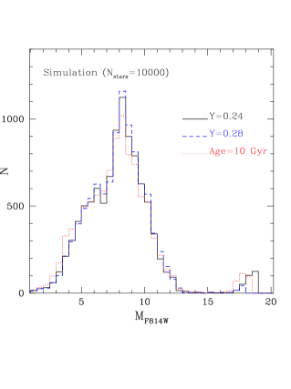
Figure 7: Theoretically predicted luminosity function for the models at Age=13 Gyr and with Z=0.0002 and two different helium abundance. A power law with exponent $\alpha$=–0.5 was used as a mass function. Also the LF at Age=10 and with Y=0.24 is shown for comparison.

The mass-luminosity relation (MLR) is essential for the comparison with the data, as it enters in the conversion of the (assumed) mass function into the luminosity function (LF).
Any change of slope of the MLR will be reflected in the luminosity function, defined as dN/dL=dN/dM $\times$ dM/dL. Where the MLR presents an inflection point, the LF has a relative maximum or minimum. As the luminosity decreases along the MS, there are two inflection points, responsible for two main peaks in the LF (see Fig.7): the first, at M_F814W $\sim$ 6 mag, is due to the transition between pure MS models and models that suffer the effects of evolution (and are more luminous in the MS due to the hydrogen consumption). Therefore, the corresponding peak in the LF is a function of age, and, we will see, of Y. After a small range of homologous models, the MLR steepens progressively due to the onset of molecular absorption in the stellar envelope; this produces a gradual increase in the LF. When models become fully convective, at $\sim$0.35M_⊙, the MLR relation begins to flatten again, and the presence of this inflection point results in the large peak at M_F814W $\sim$ 8 mag, present in all the GC LFs (D’Antona, 1998) and shown in Fig. 7.
Finally, at masses M $\sim$0.12M_⊙, the MLR relation flattens even more. This is due to the onset of degeneracy in the core of the star (D’Antona, 1998), and this latter decrease in the LF is dependent on the EOS. The HR diagram does not show the minute features of the MLR derivative, but it shows two “kinks”, the first one corresponding to the onset of molecular hydrogen dissociation in the envelope (Copeland et al., 1970) and the second to the onset of degeneracy.
In Fig. 5 we show the dependence of the MLR on the metallicity and helium content at 10 Gyr. Y influences mostly the evolved part of MS and the location of the very low masses, where degeneracy sets in and the second MS kink is located. At the MS end, decreasing the mass, the higher helium models remain more luminous and hotter. These features will affect the low luminosity LF, that will decrease more slowly with decreasing luminosity for larger Y. At the largest MS luminosities, the larger is Y, the smaller is the slope of the MLR of those models that partially burn their hydrogen during a Hubble time, with respect to the case of Y=0.24. This is an obvious feature of the evolutionary models: the larger Y produces larger MS luminosities and faster MS evolution.
The quantitative results concerning the lowest luminosities will also depend on the EOS, as we can easily understand by comparing the MLR relations obtained using EOS+OPAL and EOS+SCH tables (Fig. 6). For masses larger than 0.1M_⊙ the models using EOS+SCH are slightly more luminous, as a consequence of the differences in $\nabla_{\rm ad}$, but the trend is reversed closer to degeneracy. Obviously this variation in the slope of the MLR will produce a different shape in the peak of the LF, and in particular we expect a stronger peak when EOS+SCH are used.
An interesting theoretical feature of the models at the boundary between low mass stars and brown dwarfs is shown in Fig. 6. This figure refers to the Z=0.0002 case, for which an extended atmospheric grid is available.

Table 1: Hydrogen burning minimum mass (HBMM) for Z=0.0002 and Z=0.0006, [$\alpha$/Fe]=0, and different Y.

	Y=0.24	Y=0.28	Y=0.32	Y=0.40
Z=0.0002	0.088M⊙	0.083M⊙	0.079M⊙	0.072M⊙
Z=0.0006	0.085M⊙	0.081M⊙	0.077M⊙	0.069M⊙

In between the HBMM —the smallest mass that stabilizes in MS, in a configuration in which the total luminosity is provided by the proton–proton (p–p) reactions in the core— and the pure brown dwarfs —that never ignite the p–p chain— there is a small range of masses for which nuclear burning contributes to the stellar luminosity for even several billion years, but in the end these objects finally cool as brown dwarfs. This is a common occurrence in population I (the transition masses defined in D’Antona & Mazzitelli, 1985), where the MS merges without discontinuities into the brown dwarf cooling sequences. On the contrary, the MS of the population II has a much sharper drop, because the much smaller opacities put the HBMM at minimum luminosity a factor $\sim$10 larger, so that the transition masses cover a very small mass range. There is then a “luminosity gap” between the end of the MS and the luminosity at which the smaller brown dwarfs are able to slow their cooling down to the typical age of population II stars (10–12 Gyr). Fig. 6 translates into possible LF. In Fig.7 LFs for 10 and 13 Gyr are plotted, assuming a power law MF with exponent $\alpha$=–0.5. At 13 Gyr, the low mass brown dwarfs should emerge as a small peak at M_F814W $\sim$18, corresponding to near infrared magnitudes $\sim$30 at the distance of NGC 6397. The peak is $\sim$1 mag brighter if the age is 3 Gyr smaller. We regard this prediction as an educated guess on the possibility that the dimmest luminosities regime is populated not only by white dwarfs (Richer et al. 2008) but also by very cool brown dwarfs. However, dynamical models indicate that these objects should be preferentially stripped from the cluster. Since there is a strong difference in these two populations, as the cool white dwarfs would be located at a color M_F606W-M_F814W $\sim$1-1.2mag, while the cool brown dwarfs will not be visible in the F606W band, having M_F606W-M_F814W $\sim$5.5-7mag only future observations with even more capable telescopes should clarify the question.

5 $\alpha$-enhanced models, FG and SG populations, CNO enrichment

Table 2: Descriptions of the chemistry of the models calculated for this work.

Name	Description	Z	[C/Fe]	[N/Fe]	[O/Fe]	Reference
Z=0.0006
CNOx1s	Solar-scaled	0.0006	0.00	0.00	0.00	GS1999
CNOx1a	[$\alpha$/Fe]=0.4	0.0006	0.00	0.00	0.40	GS1999
Z=0.0002
CNOx1s	Solar-scaled	0.0002	0.00	0.00	0.00	GS1999
CNOx1a	[$\alpha$/Fe]=0.40	0.0002	0.00	0.00	0.40	GS1999
CNO$\uparrow$	total(CNO)=1.6	0.0003	0.00	1.40	0.20	this work

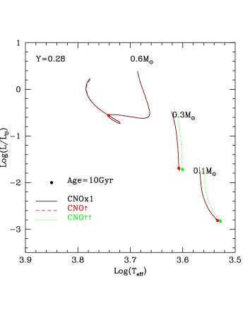
Figure 8: We show the comparison between the diagram to the standard CNO tracks at different masses(full line) and the “peculiar” ones calculated (dashed and dotted line) with the evolution of the same mass.

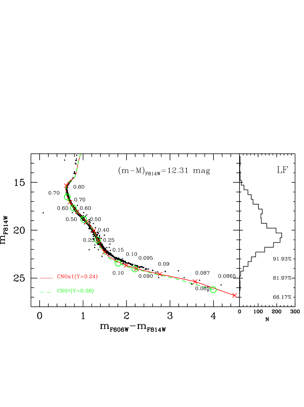
Figure 9: Left panel Main Sequence of NGC 6397 from Richer et al. (2008). Also shown are the best fit isochrones for FG (red) and SG (green) populations. Numbers indicate stellar masses (up-FG,down-SG) of same models (crosses-FG, open circle-SG) in M_⊙ units. Right panel: NGC 6397 MS Luminosity Function from data; for three low luminosities are reported the completeness fraction taken from Table 4 of Richer et al. (2008).

Comparison with low metallicity cluster stars requires use of models with $\alpha$-enhanced mixtures, for which we adopt [$\alpha$/Fe]=0.4. As discussed only up to $\sim$30$\%$ of stars of NGC 6397 can belong to the FG, the majority show indeed the Na–O anticorrelation, and many stars have very high Nitrogen content. Therefore we need also models to represent the SG. We will assume that it may differ both in helium content and in total CNO content from the standard FG. A resonable assumption for CNO is that we assume an overbundace of N by about 1.4 dex, and a variation of –0.2 dex for O, leaving carbon unchanged (A. Bragaglia, private comunication). The total “metallicity” Z in mass fraction for this CNO-enhanced mixture (CNO$\uparrow$) is now Z=0.0003. We used the OPAL Web tool to compute on purpose radiative opacities for this mixture. For T$\leq$15000K we still use the opacities by Ferguson et al. (2005) as lower temperature opacities do not affect the structure of the models we are considering. We compute on purpose radiative opacities for this mixture. All models are computed for helium mass fraction Y=0.24 and Y=0.28 and summarized in Table 2.
In general, as discussed in the analysis by Ventura et al. (2009), the largest differences between standard and CNO–enhanced mixtures are found in the ionization zone of the CNO elements, but in this case the differences are very small since the variation is not very large, and the initial abundances are very small. As a result, pratically no differences are found in effective temperature and luminosity of the models (see Fig.8).
Another possible hypothesis is that Oxygen in the SG is basically not very different from the FG value, as most of the Carretta et al. (2009a) measurements for O are only upper limits. In this case, the CNO abundance becomes even larger. In this case, we adopt as boundary conditions the grid [M/H]=–1.5. (CNO$\uparrow$$\uparrow$ models, see Table 2). As reported in Fig.8 also in this case the differences are very small but for masses of about 0.3M_⊙ the temperature are little smaller.

6 Comparison with the data of NGC 6397

We analyse both the CMD diagram and the luminosity function simulations.

6.1 Color-Magnitude diagram

In Fig. 9 we compare the models with the deep photometry of NGC 6397 by Richer et al. (2008). We plotted the isochrone that allows the best fit of both the low main sequence and the TO for the labelled value of distance modulus and reddening, with [Fe/H]=-1.99 dex (Carretta et al., 2009c) and [$\alpha$/Fe]=0.4 (solid line–red in the electronic version) and with an age of 12 Gyr which is comparable with the age obtained from the White Dwarf Cooling Sequence of NGC 6397 by Hansen et al. (2007). The distance modulus in F814W photometric band is compatible with the true distance modulus (=12.03 mag) and E(F606W-F814W)(=0.20 mag) reported in literature (see for example Table 3 of Richer et al., 2008).
As already found by Richer et al. (2008), below 0.20 M_⊙ the isochrone and the data do not match perfectly, however the data appear to terminate at about the magnitude predicted by models. We then confirm the suggestion of Richer et al. (2008) that they have observed the termination of the hydrogen burning sequence.
In Fig. 9 we also show (dashed line-green in the electronic version) the position of the isochrone obtained with models computed with Y=0.28 and CNO$\uparrow$ using the same distance modulus and age used for the FG isochrone. The two isochrones are very similar except around m_F814W=23 mag where they deviate and the FG isochrone is a little brighter. This aspect is important to understand if the tightness of the MS at this interval of magnitude depends on observational error only or is the consequence of the presence of a second generation made of stars with higher helium abundance and CNO enhancement. We select data within three different intervals of half magnitude below the MS turnoff, and rectify their colors by subtracting the color of their best-fit line, as shown in Fig. 10, left and medium panels. We do not consider the possible presence of binaries, as Davis et al. (2008) have shown that NGC 6397 has a primordial binary fraction of only $\sim$1$\%$. The histogram of the color displacements from the best fit line, shown in the right panels, are fitted with a gaussian profile with the labelled $\sigma_{obs}$.
In the same panel, for each interval of magnitude we report the color displacements for synthetic populations (assuming the distance modulus for NGC 6397 reported in Fig.9 ) under the hypothesis that the 30 $\%$ of all stars are primordial (standard helium and CNO abundance), and the restant 70 $\%$ is composed by a mixture of SG population with CNO$\uparrow$ and helium respectively up to Y=YUP=0.25, 0.26 and 0.28. As expected, the largest difference between $\sigma$ is obtained in the third interval of magnitude. From the values of dispersion reported we obtain that a SG made of stars with an helium dispersion of $\Delta$Y=0.02 is compatible with the tightness of the MS of NGC 6397.
In the case of CNO$\uparrow$$\uparrow$ models (see Section 5) the isochrone calculated for Y=0.28 overlaps exactly on the FG’s one. In this case the observational spread of MS at low magnitude may suggest an even larger spread of helium between FG and SG.

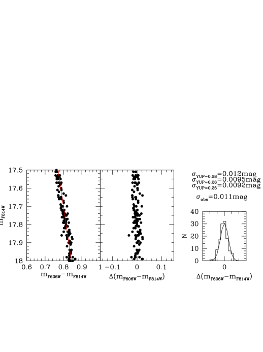
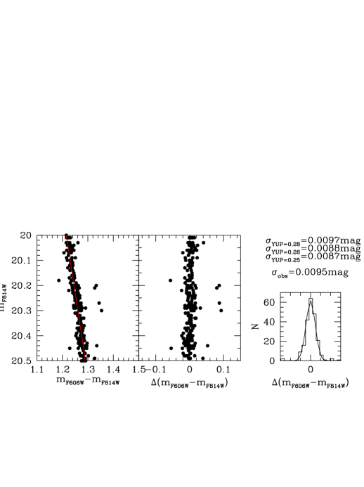
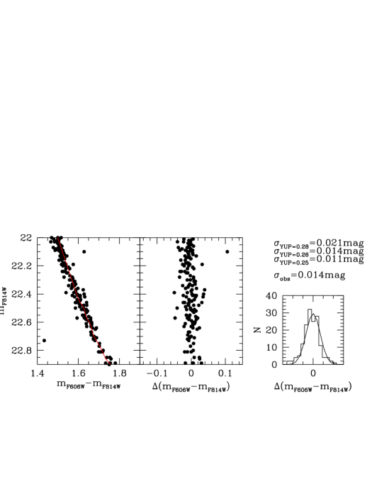
Figure 10: a) In each row a little portion of the MS of NGC 6397 is shown on the leftmost side, while in the middle panel the magnitude m_F814W is reported versus the color distance from the best–fit line. On the right panel we show the histogram of the color displacements, fitted with the best fit gaussian curve for the data. We also report the $\sigma$ of the best fit gaussian curve obtained for of synthetic population made of 30 $\%$ of stars belonging to FG and the restant 70 $\%$ made of stars of SG with different YUP.

.

6.2 Luminosity function

We now compare the observed luminosity function to the theoretical simulations. We use the magnitudes in F814W filter and derive synthetic populations from models at different ages, in the plausible range from 9 to 14 Gyr.
The mass-luminosity relation from our models was discussed in Section 4.1; now we discuss the choice of the mass function (MF). At the beginning we consider this cluster as formed by an unique population in order to define a method to compare theoretical and observational luminosity function. Due to the dynamical evolution of the cluster, the present MF is not the initial one. NGC 6397 has a collapsed core (Djorgovski & King, 1986), as it has evolved past the potentially catastrophic phase of core collapse, and is dynamically old. In particular it has been shown that NGC 6397 exhibits mass segregation, which certainly has affected the MF (Hurley et al., 2008). Silvestri et al. (1998) have shown, adopting their own low mass models and those by Baraffe et al. (1997), that the bulk of the MF can be described by a unique power law of the form dN/dM=k M^α with index ${\alpha}$=–0.5. Richer et al. (2008) found that ${\alpha}$=–0.13 gives the highest $\chi^{2}$ when comparing the models with their data of NGC 6397. They found an even better result when a lognormal distribution is used, which have the advantage to truncate the LF at the extreme low mass end but the disadvantage to introduce a new parameter.

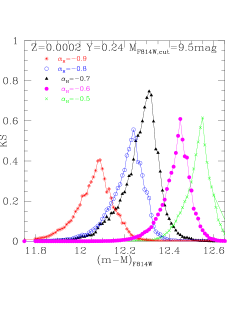
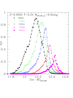
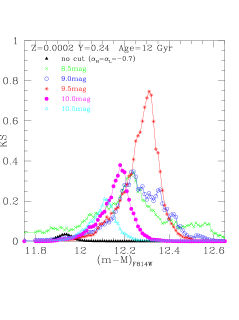
Figure 11: Distribution of KS with distance modulus for the labelled value of Z and Y and for different $\alpha_{H}$ ((upper-panel)), different ages (medium-panel) and M_F814W,cut (down-panel) (see text). In all cases a double power law was used with $\alpha_{L}$=–0.1. In the medium and down panels $\alpha_{H}$=–0.7 as inferred by the upper panel is used.

A similar result was obtained by De Marchi, Paresce & Pulone (2000)which suggested that no single power law distribution is compatible with the MS of NGC 6397; in particular they found that the MF is less steep for M$\leq$0.3M_⊙.
We simulate the synthetic populations using a power law MF with two different slopes above ($\alpha_{H}$) and below ($\alpha_{L}$) a cutoff magnitude in the range M_F814W,cut=8.5-10.5 mag (here we consider a single MF as a particular case with $\alpha_{H}$=$\alpha_{L}$.); this cutoff magnitude, for the chosen distance modulus, corresponds to a “cutoff mass”. At a fixed age, MLR gives the magnitudes of each extracted mass, according to the chosen MF, which depends by four parameter ($\alpha_{H}$, $\alpha_{L}$, M_F814W,cut and distance ). We simulate photometric errors considering gaussian errors for the magnitudes of each extracted mass in order to reproduce the width of the upper main sequence. In addition we have taken into consideration the uncertainties in completeness, by multiplying the random extractions in a given interval of masses for the completeness fractions given in Table 4 of Richer et al. (2008) and determined with the artificial star test described in Anderson et al. (2008).
We have then used the Kolmogorov-Smirnov test to compare the observed luminosity function of NGC 6397 with the theoretical one, which depends on the MF used to extract masses ($\alpha_{H}$,$\alpha_{L}$M_F814W,cut), on age and distance modulus. This statistical method has the advantage of being non-parametric and without making assumptions about the distribution function of the data, it returns the probability that two arrays of data values are drawn from the same distribution. The scalar KS (varying between 0 and 1) which give the significance level of the KS statistic i.e. the probability with which we can accept the null hypothesis. KS=1 means that the simulated and observed data follow the same function.
Another great advantage of this statistical method is that the two arrays of data does not need to have the same number of elements; this means that we can build our synthetic populations with a greater number of stars then the real stars from which we made the observed LF, making the results independent from the random extraction. We have studied the dependence of KS numbers as a function of distance modulus for each of the four free parameter (age, $\alpha_{H}$,$\alpha_{L}$ and M_F814W,cut) used to build the synthetic population and then we have compared the results in order to choice the best fit parameter. In particular as done by Richer et al. (2008) for their $\chi^{2}$ method both $\alpha_{H}$ and $\alpha_{L}$ were allowed to range from -1 and 1 in 200 steps considering. We have explored the case of a single MF as a particular case of this situation ($\alpha_{H}$=$\alpha_{L}$). We find that the best combination of power law exponents for, respectively, higher and lower masses, are $\alpha_{H}$=–0.7 and $\alpha_{L}$=–0.1. The upper panel of Fig. 11, where for example are shown the variation of KS with distance modulus for different selected $\alpha_{H}$, justify our choice. We also note that the distance modulus for which we have the higher probability is about the same distance modulus for which we have the best comparison between isochrones and CMD (see Fig.9), confirming the validity of our method. The same result is obtained using models with higher helium abundance. For these values, in Fig. 11 we also report KS as a function of distance modulus for different ages (medium panel) and for different cutoff magnitudes (lower panel). In the bottom panel, also the case of a single power law with index –0.7 is shown (black triangles): we see that a unique power law does not give a good match to the observed LF. Notice however that for higher masses this value is very different from the one obtained by Richer et al. (2008) (=–0.13). However we want too stress that this our result is consistent with their consideration that a lognormal function produces a better ${\chi}^{2}$ values than the best fitting single power law MF. In fact when a lognormal function is used one has two adjustable parameters as in our case. Concerning the age, as shown in medium panel of Fig. 11, the best agreement with observations is obtained for an age of 14-13 Gyr, but if we also consider the best distance moduli and take into account the CMD we can choose 12 Gyr together with M_F814W,cut=9.5 mag, corresponding to $M$$\sim$0.18M_⊙.
In Fig. 12 we report the NGC 6397 MS LF compared with the best fitting double power law mass functions. The overall agreement is satisfactory. Only at M_F814$\geq$12mag ($\sim$ M=0.090M_⊙), the observed stars are fewer then predicted; this may mean that the MF is even flatter at these lowest masses, due to more effective evaporation, but it may also be due to some deficiency in the models.

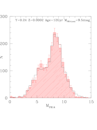
Figure 12: Comparison between observed and calculated distribution of MS stars of NGC 6397 for the labelled values of the parameters. The power law used is the same of Fig. 11. The error bars take into account the Poisson’s error and incompleteness corrections.

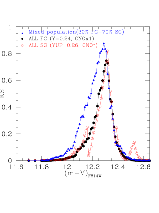
Figure 13: Distribution of KS with distance modulus for different synthetic populations.

In Fig. 13 we also show the distribution of KS in the case that 30$\%$ of stars belong to FG (Y=0.24 and CNOx1a) and 70$\%$ to the SG (YUP=0.26 and CNO$\uparrow$) which give the best match of the widht of the MS (see Fig. 10) and in the case that all stars belong to SG. The conclusion is that, since comparable KS, and reliable distance moduli are obtained in all cases, as from the widht of MS also from the luminosity function we cannot exclude that the cluster contains either a mixture of stars with different helium, or a single helium abundance for all stars.

7 Conclusions

We have computed new models for the main sequence down to the hydrogen burning minimum mass, adopting two different version of an updated equation of state and made simulations of the luminosity functions for different choices of the mass function and the initial helium content. The results are compared with the recent observations of the MS of NGC 6397 by Richer et al. (2008). Using a Kolmogorov Smirnov test to compare observed and simulated LF we found that a double power law for the mass function well reproduces the observed luminosity function in F814W photometric band. However, both the models for simple or mixed population according the spectroscopic data provide a good fit of LF. A stronger results is obtained from the analysis of the width of MS from which we find that in any case any helium variations must be confined within $\Delta$Y=0.02 in the case of CNO overabundance predicted by a mixing between 50$\%$ of pristine gas and 50$\%$ of gas eject by 5M_⊙AGB stars as suggested by Ventura $\&$ D’Antona (2009). Instead we find that a arger spread ( 0.02$\leq$$\Delta$Y$\leq$0.04) in helium between primordial and intermediate generation is compatible with the widht of main sequence when CNO$\uparrow$$\uparrow$ models are considered.

The complete sets of isochrones transformed for ACS filters F814W and F606W, calculated for this work, are available upon request to the authors and will be soon inserted on WEB at site http://www.mporzio.astro.it/$\%$7Etsa/

References

- Anderson et al. (2008) Anderson, J., King, I., Richer, H. B. et al. , 2008, AJ, 125,2114
- Alexander et al. (1997) Alexander, D.R., Brocato,E., Cassisi,S., Castellani, V., Ciacio, F., Degl’Innocenti, 1997, A&Am 317, 90-98
- Angulo et al. (1999) Angulo et al. , 1999, NuPhA., 656, 3A
- Baraffe et al. (1997) Baraffe, I. , Chabrier, G., Allard, F & Hauschildt, P H. 1997, A&A, 327, 1054
- Bedin et al. (2005) Bedin, L. R. et al. 2005, MNRAS, 357,1038
- Bessel (1990) Bessel, M., 1990, PASP, 102, 1181
- Bonifacio et al. (2002) Bonifacio, P., et al. 2002, A&A, 390, 91
- Caloi & D’Antona (2005) Caloi, V. & D’Antona, F. 2005, A&A, 121, 95
- Canuto, Goldman & Mazzitelli (1996) Canuto, V.M., Goldman, I., & Mazzitelli, I., 1996, ApJ, 473, 550
- Canuto & Mazzitelli (1991) Canuto, V. M. & Mazzitelli, I., 1991, AJ, 370, 295
- Cassisi et al. (2000) Cassisi, S.; Castellani, V.; Ciarcelluti, P.; Piotto, G.; Zoccali, M., 2000, MNRAS, 315, 679
- Cassisi et al. (2007) Cassisi, S.; Potekhin, A. Y.; Pietrinferni, A.; Catelan, M.; Salaris, M., 2007, ApJ, 661, 1094C
- Carretta et al. (2004) Carretta, E., Bragaglia, A., & Cacciari, C., 2004, ApJL, 610, L25
- Carretta et al. (2005) Carretta, E., Gratton, R. G., Lucatello, S., Bragaglia, A., & Bonifacio, P., 2005, A&A, 433, 597
- Carretta et al. (2006) Carretta, E., Bragaglia, A., Gratton, R. G., Leone, F., Recio-Blanco, A., & Lucatello, S. 2006, A&A, 450, 523
- Carretta et al. (2009a) Carretta, E., Bragaglia, A., Gratton, R. G., Lucatello, S., Catanzaro, G., Leone, F., Bellazzini, M., Claudi, R., D’Orazi, V., Momany, Y., et al, 2009a, A&A, 505, 117
- Carretta et al. (2009b) Carretta, E., Bragaglia, A., Gratton, R. G., & Lucatello, S., 2009b, A&A, 505, 539
- Carretta et al. (2009c) Carretta, E., Bragaglia, A., Gratton, R., D’Orazi, V.,. Lucatello, S., 2009c, (arXiv:0910.0675)
- Castelli & Kurucz (2004) Castelli & Kurucz, 2004, astroph 04050087 per l’ultimo aggiornamento modelli
- Catelan et al. (1998) Catelan M., Borissova J., Sweigart A.V., & Spassova N. 1998, ApJ, 494, 265
- Coc et al. (2004) Coc, A., Vangioni-Flam, E., Descouvemont, P., Adahchour, A., & Angulo, C. 2004, ApJ, 600, 544
- Copeland et al. (1970) Copeland, H.; Jensen, J. O.; Jorgensen, H., 1970, A&A, 5,12
- Chabrier & Baraffe (1997) Chabrier, G. & Baraffe, I., 1997, A&A, 1997
- Davis et al. (2008) Davis, D. S., Richer, H. B., Anderson, J.; Brewer, J., Hurley, J., Kalirai, J. S., Rich, R. M., Stetson, P. B., 2008, AJ, 135, 2155D
- D’Antona & Mazzitelli (1985) D’Antona, F. & Mazzitelli I., 1985, ApJ, 296, 502D
- D’Antona (1987) D’Antona, F. 1987, ApJ, 320, 653
- D’Antona (1998) D’Antona, F., 1998, The Stellar Initial Mass Function (38th Herstmonceux Conference), 142, 157
- D’Antona et al. (2002) D’Antona, F., Caloi, V., Montalbán, J., Ventura, P., & Gratton, R. 2002, A&A, 395, 69
- D’Antona & Caloi (2004) D’Antona, F., & Caloi, V. 2004, 611, 871
- D’Antona & Caloi (2008) D’Antona, F., & Caloi, V. 2008, MNRAS, 390, 693
- Decressin et al. (2007) Decressin, T., Meynet, G., Charbonnel, C., Prantzos, N., & Ekström, S. 2007a, A&A, 464, 1029
- De Marchi, Paresce & Pulone (2000) De Marchi, G., Paresce, F. & Pulone L., 2000, ApJ,530, 342
- de Mink et al. (2009) de Mink, S. E., Pols, O. R., Izzard, R., & Yoon, S.-C. 2009, A&A, in press
- D’Ercole et al. (2008) D’Ercole, A., Vesperini, E., D’Antona, F., McMillan, S. L. W., & Recchi, S. 2008, MNRAS, 391, 825
- Di Criscienzo, Ventura & D’Antona (2008) Di Criscienzo, M., Ventura, P.& D’Antona, F., 2008, A&A, accepted (arXiv0812.3838C)
- Djorgovski & King (1986) Djorgovski, S. & King, I. R., ApJ, 305, L61
- Dotter (2007) Dotter, A., 2007, PhD Thesis
- Dotter et al. (2007) Dotter , A., Chaboyer, B., Jevremovic, D., Baron, E., Ferguson, J. W., Sarajedini, A. & Anderson, J., 2007, AJ, 134, 376
- Ferguson et al. (2005) Ferguson J. W., Alexander D. R., Allard F. et al., 2005, ApJ, 623, 585
- Fontaine et al. (1977) Fontaine, G., Graboske, H. C., Jr., & van Horn, H. M. 1977, ApJS, 35, 293
- Gratton et al. (2001) Gratton, R. G., Bonifacio, P., Bragaglia, A., et al., 2001, A&A, 369, 87
- Gratton et al. (2003) Gratton, R. G. et al., 2003, A&A, 408, 529G
- Grevesse & Sauval (1999) Grevesse, N. & Sauval, A. J., 1999, A, 347, 348G
- Hauschildt, Allard & Baron (1999) Hauschildt, P. H., Allard, F., & Baron, E., 1999, ApJ, 512, 377
- Heiter et al. (2002) Heiter U., Kupka F., van’t Veer-Menneret C., Barban C., Weiss W.W., Goupil M.-J., Schmidt W., Katz D., Garrido R., 2002, A&A 392, 619-636
- Hansen et al. (2007) Hansen, B., Anderson, J., Brewer, J. et al. , 2007, ApJ, 671, 380
- Hurley et al. (2008) Hurley, R. J., etc…, 2008, AJ, 135.2129
- Iglesias & Rogers (1996) Iglesias C. A. & Rogers F. J., 1996, ApJ, 464, 943
- Irwin (2004) Irwin, A., 2004, Technical Report http://freeeos.sourceforge.net/
- Johnson & Bolte (1998) Johnson J.A., & Bolte M. 1998, AJ, 115, 693
- King et al. (1998) King, I. R., Anderson, J., Cool, A. M., & Piotto, G. 1998, ApJ, 492, L37
- Korn et al. (2007) Korn, A. J., Grundahl, F.,Richard, O., Mashonkina, L., Barklem, P. S., Collet, R., Gustafsson, B., & Piskunov, N. 2007, ApJ, 671, 402
- Lee et al. (1994) Lee Y.-W., Demarque P., & Zinn R. 1994, ApJ, 423, 248
- Lind et al. (2009) Lind, K., Primas, F., Charbonnel, C., Grundahl, F., Asplund, M.,2009A&A,503,545L
- Kroupa, Tout & Gilmore (1993) Kroupa, P., Tout, C. A. & Gilmore, G., 1993, MNRAS, 262, 545
- Kroupa (2002) Kroupa, P., 2002, Science, 295,82
- Magni & Mazzitelli (1979) Magni, G., & Mazzitelli, I. 1979, A&A, 72, 134
- Milone et al. (2008) Milone, A. P., et al., 2008, ApJ, 673, 241
- Montalban, D’Antona & Mazzitelli (2000) Montalban, J., D’Antona, F. & Mazzitelli, I., 2000, A&A, 360,935
- Montalbán et al. (2001) Montalbán, J., Kupka, F., D’Antona, F., & Schmidt, W. 2001, A&A, 370, 982
- Montalbán et al. (2004) Montalbán, J., D’Antona, F., Kupka, F., & Heiter, U. 2004, A&A, 416, 1081
- Paresce, De Marchi & Romaniello (1995) Paresce, F., De Marchi, G. & Romaniello, M., 1995, ApJ, 440. 216
- Pasquini et al. (2008) Pasquini, L., Ecuvillon, A., Bonifacio, P., & Wolff, B. 2008, A&A, 489, 315
- Piotto et al. (2007) Piotto, G., et al.,2007, ApJ Letters, 661, L53
- Potekhin et al. (1999) Potekhin, A. Y.; Baiko, D. A.; Haensel, P.; Yakovlev, D. G., 1999, A&A, 346, 345P
- Pumo et al. (2008) Pumo, M. L., D’Antona, F., & Ventura, P. 2008, ApJ, 672, L25
- Ramírez & Cohen (2002) Ramírez, S. V., & Cohen, J. G. 2002, AJ, 123, 3277
- Rey et al. (2001) Rey S.C., Yoon S.J., Lee Y.W., Chaboyer B., & Sarajedini A. 2001, AJ, 122, 3219
- Richer et al. (2006) Richer, H. B., et al., 2006, Science, 313, 936
- Richer et al. (2008) Richer, H. et al., 2008, AJ, 135,2141
- Rogers et al. (1996) Rogers, F. J., Swenson, F. J., & Iglesias, C. A. 1996, ApJ, 456, 902
- Sarajedini et al. (2007) Sarajedini,A. et al., 2007, AJ, 133,1658
- Saumon, Chabrier & van Horn (1995) Saumon, D., Chabrier, G., van Horn H.M., 1995, ApJS 99, 713
- Silvestri et al. (1998) Silvestri, F., Ventura, P., D’Antona, F., Mazzitelli, I., 1998, A&A, 334, 953
- Sirianni et al. (2005) Sirianni, M., et al. 2005, PASP,117,1049
- Stolzmann & Blöcker (2000) Stolzmann W., Blöcker T., 2000, A&A, 361, 1152
- Vandenberg & Clem (2003) Vandenberg, D. A. & Clem, 2003, AJ, 126, 778
- Ventura et al. (2001) Ventura, P., D’Antona, F., Mazzitelli, I., & Gratton, R. 2001, ApJ Letters, 550, L65
- Ventura, D’Antona & Mazzitelli (2007) Ventura P., D’Antona, F. & Mazzitelli I., 2007, Ap&SS, 420
- Ventura et al. (2009) Ventura, P.; Caloi, V.; D’Antona, F.; Ferguson, J.; Milone, A.; Piotto, G. P., 2009, MNRAS, 399, 934
- Ventura & D’Antona (2009) Ventura, P. & D’Antona, F., A&A, 499, 835