The Ratio of Luminous to Faint Red Sequence Galaxies in X-ray and Optically Selected Low-Redshift Clusters

Abstract

We study the ratio of luminous-to-faint red sequence galaxies in both optically and X-ray selected galaxy clusters in the poorly studied redshift range $0.05\leq z<0.19$. The X-ray selected sample consists of 112 clusters based on the ROSAT All-Sky Survey, while the optical sample consists of 266 clusters from the Sloan Digital Sky Survey. Our results are consistent with the presence of a trend in luminous-to-faint ratio with redshift, confirming that downsizing is continuous from high to low redshift.
After correcting for the variations with redshift using a partial Spearman analysis, we find no significant relationship between luminous-to-faint ratio and X-ray luminosity of the host cluster sample, in contrast to recent suggestions. Finally, we investigate the stacked colour-magnitude relations of these samples finding no significant differences between the slopes for optically and X-ray selected clusters. The colour-magnitude slopes are consistent with the values obtained in similar studies, but not with predictions of theoretical models.

1 INTRODUCTION

It is still unclear how galaxies evolve over the Hubble time and the picture is complicated because galaxy properties also depend on environment and mass. In fact, although these dependencies have been extensively studied, it is still an open question as to how they are related to the evolution we see. An excellent probe of this evolution is the colour-magnitude relation (CMR) of early-type galaxies in clusters and groups, first noted by Visvanathan & Sandage (1977) and interpreted as a correlation between galaxy mass and mean stellar metallicity (Kodama & Arimoto, 1997). The morphology of the CMR is observed to evolve with redshift and its origin can be explained either through concurrent formation of elliptical galaxies in cluster cores in a high redshift monolithic collapse (Kodama & Arimoto, 1997) or, alternatively, through the hierarchical formation of elliptical galaxies via merging over cosmic time (Kauffmann & Charlot, 1998).
The reliability and the utility of the CMR as a probe of galaxy evolution has also been highlighted by the fact that it is an extremely good tool for the identification of galaxy structures like clusters and groups (see e.g. Gladders et al., 1998; Koester et al., 2007; Swinbank et al., 2007; Capozzi et al., 2009). Evaluating the relative number of faint and luminous red-sequence galaxies (RSGs) in clusters as a function of redshift (De Lucia et al., 2004, 2007; Stott et al., 2007; Gilbank & Balogh, 2008) and environment (Tanaka et al., 2005), is an effective method with which to investigate how galaxies evolve towards the CMR. The tools used to quantify the evolution of the red sequence are the faint-end slope of the red-sequence luminosity function and the ratio of the number of luminous to faint galaxies (lum/faint or, alternatively, giant to dwarf, g/d) on the CMR. There is a current debate concerning which of these two tools is best for undertaking these kinds of studies. For instance, Andreon (2008) argued that the use of the faint-end slope is preferable, since it is a measure of the lum/faint ratio, it is easier to deal with from a statistical point of view and has the advantage of using all the data available. On the other hand, Gilbank & Balogh (2008) pointed out that the dwarf to giant (d/g) ratio is just a luminosity function reduced to two bins and avoids the complication of having to fit an analytic function, which usually involves degeneracies between the fitted parameters.

Previous studies carried out to investigate the lum/faint ratio as a function of redshift have provided conflicting results. Some of them (Barkhouse et al., 2007; Stott et al., 2007; De Lucia et al., 2007; Gilbank et al., 2008; Hansen et al., 2009) showed results consistent with an increasing trend of the lum/faint ratio with redshift, while other studies (Tanaka et al., 2005; Andreon, 2008) indicated that the cluster lum/faint ratio may not evolve with redshift. Tanaka et al. (2005), using three clusters at different redshifts (0, 0.55 and 0.89) found a discordant result only for their $z\sim 0$ cluster, while Andreon (2008), studying 28 clusters at $0.02<z<1.3$ individually, concluded there is no evolution with z. A quite different scenario is the one found by Lu et al. (2009). In their study of 127 Canada-France-Hawaii Telescope Legacy Survey (CFHTLS) rich clusters with $0.17\leq z\leq 0.36$, in comparison with Coma cluster and a sub-sample of 22 groups with $0.08<z<0.09$ taken from the group catalogue by Yang et al. (2007), they found no strong evolution of the d/g ratio (or, similarly, of the faint end of the luminosity function) over the redshift window $0.2\lesssim z\lesssim 0.4$. On the other hand, they also report an increase of a factor of $\sim 3$ from $z\sim 0.2$ to $z\sim 0$.

Several studies have investigated the dependence of the lum/faint ratio on the mass of the host systems, by looking for trends with cluster richness, velocity dispersion or X-ray luminosity. Unfortunately these studies have also led to contradictory results. Hansen et al. (2009) and Gilbank et al. (2008) found that the faint-end slope of the cluster red-sequence luminosity function depends on cluster richness for $z\lesssim 0.5$, such that low-mass clusters have higher g/d ratios than richer systems. According to the findings of De Lucia et al. (2007), at intermediate redshifts (0.4-0.8), the lum/faint ratios of clusters with velocity dispersion larger than $600\ {\rm{km\ s^{-1}}}$ appear to be larger than those measured for clusters at the same redshift but with lower velocity dispersion. However, De Lucia et al. (2007) pointed out that the error bars and the cluster-to-cluster variations were too large to draw any definitive conclusions regarding this point. On the other hand, Gilbank & Balogh (2008), using data from three different cluster samples all at $z\sim 0.5$ (De Lucia et al., 2007; Stott et al., 2007; Gilbank et al., 2008), suggested that the g/d ratio is relatively insensitive to mass or selection method over the mass range covered by the analysed clusters. They also suggested that the evolution of the cluster g/d ratio is not due to a systematically changing mass limit with redshift. However, their findings are probably the result of a sample built largely from only massive clusters. In fact, only when comparing clusters with large differences in mass (e.g., De Lucia et al., 2007; Gilbank et al., 2008 and generally with optically selected samples) is a trend likely to be seen. Turning to the studies involving clusters investigated individually, where the cluster-to-cluster scatter is larger than cases where at least tens of clusters per redshift bin are used, Koyama et al. (2007) analysed three X-ray selected clusters. They studied how the faint-end slope of the luminosity function varied with cluster X-ray luminosity ($L_{\rm X}$), finding quite a steep trend. However, this trend, as mentioned by Koyama et al. themselves, is largely based on a sample of inadequate size, given the large intrinsic scatter. Finally, Andreon (2008), using a sample of 28 X-ray selected clusters, found no correlation between lum/faint ratio and either $L_{\rm X}$ or velocity dispersion, obtaining the same result utilizing the faint-end slope of the luminosity function.

Our work aims to study the evolution of red galaxies in optically and X-ray selected galaxy clusters using data from the Sloan Digital Sky Survey Data Release 6 (SDSS DR6), in order to investigate how the lum/faint ratio varies between different cluster samples (optical and X-ray) and to investigate possible trends with cluster mass and redshift. To parametrize the build up of the CMR, we focus our attention on the lum/faint ratios and the colour-magnitude relations obtained for two cluster samples, one optically selected from SDSS data and the other X-ray selected from the ROSAT All-Sky Survey data (RASS). We decided to use the lum/faint ratio as an estimate of the relative number of luminous and faint RSGs, since this is independent on the form of the luminosity function. We perform our study of the lum/faint ratio in a poorly studied redshift interval ($0.05\leq z<0.19$) (few studies, e.g. Barkhouse et al., 2009 and Lu et al., 2009 have investigated similar redshift windows), as most of the previous studies have focused either on the intermediate and high redshift regime ($0.4\lesssim z\lesssim 1.0$) or on Coma-like redshifts ($z\sim 0.02$).

The paper is structured as follows: in Sect. 2 we describe the cluster samples and the data used in the analysis, while Sect. 3 is dedicated to the data analysis. Sects. 4 and 5 are focused on the stacked CMRs and on the dependence of the lum/faint ratio with redshift, richness, cluster centric distance and $L_{\rm X}$, while in Sects. 6 and 7 we present and discuss the results. Finally, in Sect. 8 we draw our conclusions.
Throughout this paper we make use of magnitudes in the AB photometric system and assume a standard cosmology with $H_{0}=70\ {\rm km\ s^{-1}\ Mpc^{-1}}$, $\Omega_{m}=0.3$ and $\Omega_{\lambda}=0.7$.

Figure 1: Sky distribution of eBCS (Ebeling et al., 1998; Ebeling et al., 2000) and Bahcall et al. (2003) cluster samples (black and cyan dots, respectively) superimposed on the SDSS DR6 footprint (grey background). An Aitoff projection in equatorial coordinates is used. The eBCS sample (from which our eBCS subsample is extracted) is made of 310 X-ray selected clusters covering a redshift range of $0.02\lesssim z\lesssim 0.42$. The Bahcall et al. (2003) cluster sample (from which our optical subsamples B and HB are extracted) is made of 799 optically selected clusters covering a redshift range of $0.05<z<0.3$.

2 SAMPLE SELECTION & DATA

To perform our study, we utilize two cluster samples composed of X-ray and optically selected systems, respectively; their sky distribution, superimposed on the SDSS DR6 footprint, and the redshift distribution are shown in Figs. 1 and 2, respectively.

The X-ray selected cluster sample contains 112 clusters with $0.05\leq z<0.19$ falling into the SDSS DR6 footprint, included in the homogeneously selected extended Brightest Cluster Sample (eBCS, Ebeling et al., 1998; Ebeling et al., 2000). This sample is made up of two cluster catalogues both selected from the RASS data in the northern hemisphere ($\delta\geq 0\ {\rm deg}$) and at high Galactic latitudes ($|b|\geq 20\ {\rm deg}$): (i) a 90 per cent flux-complete sample (called the ROSAT Brightest Cluster Sample, BCS) consisting of the 201 X-ray brightest clusters in the RASS data, with measured redshifts $z\leq 0.3$ and fluxes higher than $4.4\times 10^{-12}\ {\rm erg\ cm^{-2}\ s^{-1}}$ in the $0.1-2.4\ {\rm keV}$ band; (ii) a low-flux extension of the BCS comprising 107 X-ray clusters of galaxies with measured redshifts $z\leq 0.42$ and total fluxes between $2.8\times 10^{-12}$ and $4.4\times 10^{-12}\ {\rm erg\ cm^{-2}\ s^{-1}}$ in the $0.1-2.4\ {\rm keV}$ band (the latter value being the flux limit of the original BCS).
X-ray fluxes have been computed using an algorithm tailored for the detection and characterization of X-ray emission from galaxy clusters (Ebeling et al., 2000) and the fluxes are accurate to better than 15 per cent ($1\sigma$ error). The nominal completeness of the eBCS sample, defined with respect to a power-law fit to the bright end of the BCS $\log{N}-\log{S}$ distribution (see Fig. 2 in Ebeling et al., 2000), is 75 per cent, compared with 90 per cent for the high-flux BCS.
We use the fluxes published in Ebeling et al. (1998); Ebeling et al. (2000) to calculate cluster X-ray luminosities according to the cosmological model used in this work.

Sample	slope	$\mathbf{z\ bin_{1}}$	$\mathbf{\rm{\bf lum_{1}}}\|\mathbf{\rm{\bf faint_{1}}}$	$\mathbf{\rm{\bf lum/faint_{1}}}$	$\mathbf{z\ bin_{2}}$	$\mathbf{\rm{\bf lum_{2}}}\|\mathbf{\rm{\bf faint_{2}}}$	$\mathbf{\rm{\bf lum/faint_{2}}}$
eBCS	$-0.036^{+0.001}_{-0.001}$	0.08	$25\|45\$	$0.47\pm 0.01$	0.15	$34\|56\$	$0.60\pm 0.02$
B	$-0.035^{+0.003}_{-0.002}$	0.09	$12\|22\$	$0.46\pm 0.02$	0.16	$13\|22\$	$0.52\pm 0.02$
HB	$-0.032^{+0.002}_{-0.003}$	0.08	$13\|25\$	$0.41\pm 0.02$	0.15	$14\|25\$	$0.43\pm 0.02$

Table 1: Values of stacked CMR slope (see Fig. 3), average number of luminous and faint RSGs per redshift bin and background corrected lum/faint ratio (see Fig. 4) per redshift bin for the analysed cluster samples. The lum/faint ratio calculated in the background fields is always comprised between 0.19 and 0.22. The error values of the slopes correspond to the 95 per cent confidence interval as measured on the bootstrap distributions.

The optically selected cluster sample is the one presented by Bahcall et al. (2003) containing 799 clusters of galaxies in the redshift range $z=0.05-0.3$ and selected from $\sim 400\ {\rm deg^{2}}$ of early SDSS commissioning data along the celestial equator. Clusters have been found through the application of two independent identification algorithms: a colour-magnitude red-sequence maxBCG technique (Koester et al., 2007) and a hybrid matched filter method (hereafter HMF, Kim et al., 2002). These two algorithms focus on different properties of galaxy clusters. The maxBCG uses a brightest cluster galaxy (BCG) likelihood based on luminosity and colour applied to each SDSS galaxy weighted by the number of nearby galaxies located within the CMR appropriate to E and SO galaxies. The algorithm therefore selects clusters dominated by bright red galaxies. In contrast the HMF uses a model Plummer density profile and a Schechter luminosity function (Schechter, 1976) with typical parameters observed for galaxy clusters and is sensitive to the galaxy population fainter than $L^{\ast}$. The use of both maxBCG and HMF selected clusters enables us to include determinations of the CMR for representative cluster selection algorithms based on galaxy colour and density profile. The optical sample contains clusters with richness $\Lambda\geq 40$ (HMF richness) and $N_{gal}\geq 13$ (maxBCG richness), which translates into a mean cluster velocity dispersion of $\sigma_{r}\gtrsim 400\ {\rm{kms^{-1}}}$.
We refer to the original papers for a detailed description of these two algorithms.

For our analysis we utilize the SDSS DR6 public archive, which covers $9,583\ {\rm deg^{2}}$ of the celestial sphere in 5 bands (ugriz).

Figure 2: Redshift distribution of the analysed clusters taken from eBCS (Ebeling et al., 1998; Ebeling et al., 2000) and Bahcall et al. (2003) cluster samples.

3 Analysis

For the clusters in all samples we extract photometric data from the SDSS DR6 data base. We exclude clusters located at the borders of the DR6 footprint and select only clusters in the redshift range $z=0.05-0.19$, where the highest z is chosen to remain within the magnitude completeness level of SDSS. So, we are finally left with 112 (eBCS sample) and 266 (optical sample) clusters. We split the optical sample into two subsamples according to the selection method used: B subsample (181 clusters) containing maxBCG clusters; HB subsample (156 clusters) made of HMF clusters. These two subsamples partially overlap (71 B clusters are included in the HB subsample).
In our analysis we use the dereddened model magnitudes from SDSS, corrected for AB offsets. To perform k corrections we always utilize the software developed by Blanton & Roweis (2007) for creating template sets based on stellar population synthesis models from a set of heterogeneous photometric and spectroscopic galaxy data. The technique, suitable for estimating k corrections for ultraviolet, optical and near infrared observations in the redshift range $0<z<1.5$, is based on the non-negative matrix factorization method, which is akin to principal component analysis. The templates are fitted to data from Galaxy Evolution Explorer (GALEX), SDSS, Two-Micron All Sky Survey (2MASS), the Deep Extragalactic Evolutionary Probe (DEEP) and the Great Observatories Deep Survey (GOODS). We refer to the original paper for further details. We always use the values of Poggianti (1997) to correct for passive evolution.

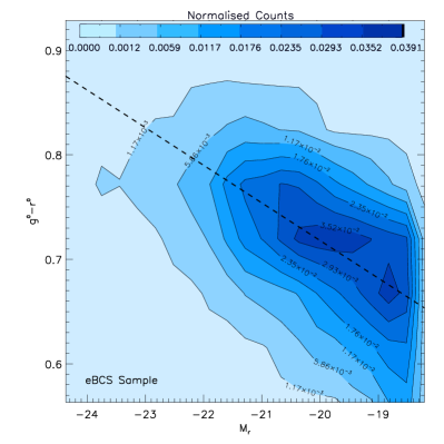
Figure 3: Density maps of the stacked g-r vs. $M_{\rm r}$ colour-magnitude diagrams for eBCS (upper left panel), B (upper right panel) and HB (lower panel) samples. All counts per bin (of sides 0.3 in magnitude and 0.05 in colour) are normalized to the value of the total counts. Isodensity contour levels are superimposed and colour coded (the lighter the colour, the less counts) according to the colour bar in the plots. The best-fitting CMR (dashed line) is superimposed.

4 Colour-Magnitude Relation

We obtain the stacked g-r vs. r CMR for all the analysed samples (Fig. 3), using red galaxies within $1\ {\rm Mpc}$ from the cluster centroids in the cluster’s rest-frame. We first apply a k correction and calculate distances assuming all galaxies are at their cluster’s mean redshift. Then we perform a biweight fit (Beers et al., 1990) on the stacked colour-magnitude diagram using all galaxies with $M_{r}\leq-21$ (this limit is chosen in order to avoid excess noise in the CMR). From this, we obtain an estimate of the slope and the zero-point of the stacked CMR. The biweight fit is performed iteratively using only those galaxies located within $0.2\ {\rm mag}$ of the previous CMR best-fitting line.
To correct for passive evolution, we use the trends given by Poggianti (1997) for the redshift range used in this study ($0.05\leq z<0.19$). Over this interval, the correction is virtually linear and is almost independent of the morphological type. The correction is calculated by means of a linear interpolation between the values given by Poggianti and converted to the r band. Only galaxies within $\pm 0.1\ {\rm mag}$ of the CMR best-fitting line are corrected for passive-evolution, to minimize contamination by blue galaxies. Subsequently, we perform the last biweight fit using only passive-evolution corrected galaxies (Fig. 3) to obtain a final CMR best-fitting line. To measure the accuracy of the best-fitting CMR parameters, we adopt a bootstrap technique and resample, with replacement, the clusters constituting the stacked colour-magnitude distribution 1000 times. By carrying out the same biweight fit we derive the marginalized 2-$\sigma$ confidence levels on the measured parameters from their bootstrap distributions. We perform this analysis on all the cluster samples (eBCS, B, BH). The final results for the CMR slope are reported in Tab. 1.

5 Luminous to Faint Ratios

Following the approach used by De Lucia et al. (2007), we split the galaxies on the red sequence into luminous (or giant) and faint (or dwarf) galaxies for each cluster. De Lucia et al. (2007) classify all galaxies having $M_{\rm{V}}<-20$ as luminous and those galaxies with $-20<M_{\rm{V}}<-18.2$ as faint; these limits are valid for galaxies whose magnitudes have been corrected for passive evolution to z = 0. The Johnson V band magnitude can be computed from SDSS photometry using the following relation:

$$V=r+0.44*(g-r)-0.02,$$ (1)

which has an accuracy better than 0.05 mag (Fukugita et al., 1996). We use this transformation to convert the De Lucia et al. magnitude limits from V to r band, utilizing the colour $g-r=0.77$ computed by Fukugita et al. (1995) for an elliptical galaxy at z = 0. After this transformation, we obtain a faint and a bright absolute magnitude limit of $M_{\rm{r}}=-18.52$ and $M_{\rm{r}}=-20.32$ respectively. To calculate the number of faint and luminous galaxies on the colour-magnitude relation of our clusters, we perform a biweight fit (Beers et al., 1990) on the apparent colour-magnitude diagram (g-r vs. r) of each cluster to determine an individual best-fitting CMR, using only galaxies within $1\ {\rm Mpc}$ of the cluster centroids.
Hereafter RSGs refer to galaxies within $\pm 0.3\ {\rm mag}$ of each individual CMR best-fitting line. To determine the number of faint and luminous RSGs, we need to transform the faint and luminous absolute magnitude limits previously discussed, into apparent magnitudes (hereafter $m_{\rm{faint}}$ and $m_{\rm{lum}}$). We perform this transformation using a mean k correction value calculated by averaging all the galaxies within $1\ {\rm Mpc}$ of the cluster centroids and applying a passive-evolution correction inferred as in Sect. 4. At this point, we determine the number of faint ($m_{\rm{lum}}\leq m_{\rm{r}}\leq m_{\rm{faint}}$) and luminous ($m_{\rm{r}}<m_{\rm{lum}}$) RSGs per cluster within $0.75\ {\rm Mpc}$ of their centroids.
Note that the choice of a radial distance of $0.75\ {\rm Mpc}$ is taken in order to be consistent with the analysis performed by De Lucia et al. (2007).
The canonical photometric completeness limit of SDSS is defined as the 95 per cent detection repeatability for point sources (g=22.2; r=22.2, as reported on SDSS website). However, the extended profile of early-type galaxies outside the point spread function may result in incompleteness at a brighter magnitude limit. In order to estimate the completeness level, we use Cross et al. (2004), who studied the completeness of SDSS Early Data Release by comparing galaxy number counts as a function of surface brightness, using the overlapping region of the deeper Millennium Galaxy Catalogue. For galaxies with $\mu_{50_{\rm r}}\lesssim 24.6$ the completeness is $>95$ per cent, while for galaxies with $24.6\lesssim\mu_{50_{\rm r}}\lesssim 25.6$ it reduces to $\sim 90$ per cent. Using the same definition of surface brightness of Cross et al. (2004), for our data in the highest redshift interval ($0.15<z<0.19$) this translates to losing a fraction of faint galaxies with $24.6\lesssim\mu_{50_{\rm r}}\lesssim 25.6$ corresponding to the 0.5 per cent of the total number of faint galaxies. Therefore, we think the effect of incompleteness is negligible and does not affect our results.

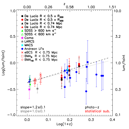
Figure 4: Luminous-to-faint ratios as function of redshift [$\log({\rm lum/faint})$ vs. $\log(1+z)$] obtained using the mean background method. De Lucia et al. (2007) values: $R<0.5\times R_{200}$ (black and red plain dots), $R<0.74\ {\rm{Mpc}}$ (black and red plain triangles), SDSS clusters with $\sigma_{\rm{r}}>600\ {\rm{km\ s^{-1}}}$ (plain green triangle), SDSS clusters with $\sigma_{\rm{r}}<600\ {\rm{km\ s^{-1}}}$ (open green triangle), Coma cluster (magenta plain star). Stott et al. (2007) values: LARCS (grey plain star), MACS (cyan plain star). Blue full dots represents Andreon (2008) values. Red asterisks, crosses and plain squares represent our values for eBCS, HB and B samples respectively. Red symbols have been inferred through a statistical approach, while black ones have been derived through the application of photometric redshifts. The best-fitting line obtained through a weighted fit carried out excluding values inferred through individual cluster measurements is plotted (dashed black line). The dotted grey line is obtained when the single cluster measurements are included (in both cases clusters from Andreon (2008) with $z>1$ are excluded, see the text). The errors on the slopes are evaluated through a jackknife technique.

5.1 Background Subtraction

We utilize two approaches to evaluate the numbers of background galaxies contaminating the estimates of faint and luminous RSGs. The first one makes use of 17 control fields (De Filippis et al., 2009, in preparation), randomly selected within the SDSS footprint, within which, after an a posteriori check, no large local structures are found (Tab. 2, total area of $16.36\ {\rm deg^{2}}$). We determine the number of faint and luminous galaxies within $\pm 0.3\ {\rm mag}$ from the cluster CMR in each background region and after normalising them for the area, we calculate a weighted mean of the obtained values. The second approach, utilizes a local background, i.e. an annular region between 2 and 3 Mpc. The numbers of faint and luminous galaxies are determined in the same way as the mean background approach. Comparing the final background subtracted distributions of lum/faint ratios for the two methods we obtain very similar results within $1\sigma\sim 0.03$ and therefore in what follows we present the results only for the mean background method.

bgID	RA (degrees)	Dec (degrees)	radius (arcmin)
BG00001	180.0	54.0	21.0
BG00002	170.0	53.0	35.0
BG00003	120.0	12.0	60.0
BG00004	120.0	14.0	22.0
BG00005	120.0	20.0	27.0
BG00006	120.0	22.0	19.0
BG00007	120.0	26.0	23.0
BG00008	125.0	24.0	21.0
BG00009	125.0	26.0	21.0
BG00010	130.0	24.0	55.0
BG00011	130.0	20.0	20.0
BG00012	140.0	22.0	47.0
BG00013	140.0	20.0	24.0
BG00014	240.0	42.0	23.0
BG00015	230.0	40.0	37.0
BG00016	230.0	52.0	40.0
BG00017	315.0	0.0	28.0

Table 2: Control fields used for the background subtraction (De Filippis et al., 2009, in preparation).

5.2 Dependence on Redshift, Radius, Richness and $\mathbf{L_{X}}$

To study the relationship between lum/faint ratios and redshift we subdivide clusters in two redshift bins. In each of these bins, we then calculate a weighted mean of their ratios (Tab. 1). A potential problem is that, below $z\sim 0.1$, the $4000\ {\rm\AA}$ break is beginning to slip to the extreme blue edge of the g filter (at our minimum redshift of 0.05, the Balmer break falls at $\sim 4200\ {\rm\AA}$ whereas the g filter’s waveband starts approximately at $4000\ {\rm\AA}$), potentially biasing our estimates of the ratios in the lowest redshift bin. We test this possibility by recalculating the ratios in this redshift bin using the u-r filter combination. For the eBCS sample, for instance, we obtain a value of ${{\rm lum/faint}_{1}}=0.46\pm 0.02$, very similar to the value obtained for the same sample using the g-r colour, which is ${{\rm lum/faint}_{1}}=0.47\pm 0.01$.
We compare our results (Fig. 4) together with other literature estimates over the redshift range $0.02<z<1.3$.
We also investigate the presence of a trend of the lum/faint ratio with cluster-centric distance, since, as highlighted recently by Barkhouse et al. (2009), the use of a fixed physical aperture, instead of one scaled to the cluster’s virial radius, may cause the lum/faint ratios to be over estimated for more massive clusters. However, our adopted radius of $0.75\ {\rm Mpc}$ covers a fraction of the virial radius in $0.3\lesssim\frac{0.75\ {\rm Mpc}}{r_{\rm vir}}\lesssim 0.5$ for the eBCS sample, over which the lum/faint ratio should not evolve significantly (Fig. 2 of Barkhouse et al., 2009). For similar reasons, we do not expect these issues to significantly affect the optical sample either. However, since our methodology of estimating the lum/faint ratio and the one used by Barkhouse et al. (2009) might not be directly interchangeable, we further investigate its trend with cluster-centric distance. In order to highlight differences, we test the change of the lum/faint ratio with radius by recalculating its values using an aperture of $1.5\ {\rm Mpc}$ (corresponding to $0.6\lesssim\frac{1.5}{r_{\rm vir}}\lesssim 1$ for the eBCS sample). We find no significant differences in the values of the lum/faint ratio (e.g., for the B sample, in order of increasing z: 0.47, 0.52).
In addition, we study the relation between lum/faint ratio and cluster richness looking for correlations between lum/faint and lum RSGs and between lum and faint RSGs. For this purpose we use both the full scatter plots and the ones obtained for each redshift bin. When performing Spearman’s rank correlation tests on these plots, no significant correlation is found (r values are always about 0.4 for lum/faint vs. lum correlation and 0.5 for lum vs. faint correlation).
Finally, in order to further investigate the dependence of the lum/faint ratio on cluster mass, we study it as a function of $L_{\rm X}$ for the eBCS sample. We subdivide this sample according to z and $L_{\rm X}$ in order to obtain approximately equally populated volume limited bins (Fig. 5). We then analyse the ratio as a function of $L_{\rm X}$ in each redshift bin. Our results are shown in Fig. 6, where a mass scale is also shown, inferred by using the $M_{\rm 200}-L_{\rm X}$ relation of Popesso et al. (2005).

6 Results

Our study of the lum/faint ratio yields statistical results for all three of our samples which are consistent with those found by De Lucia et al. (2007) for SDSS clusters (Fig. 4). We test the correlation of lum/faint ratio with z [in terms of $\log({\rm lum/faint})$ and $\log(1+z)$] by performing a Spearman rank correlation test on only the values based on cluster samples (De Lucia et al., 2007; Stott et al., 2007 and this work). We find a rank correlation coefficient of $0.89$ with a two sided significance of its deviation from zero of $4\times 10^{-8}$. We also perform a weighted fit on the same points plotted in Fig. 4 (dashed line), obtaining a slope of $1.2\pm 0.1$. The error is obtained through a jackknife technique, in order to probe the stability of the trend. In determining the best fit, we prefer to exclude the lum/faint ratio values obtained for individual clusters (the values of Andreon, 2008 and of De Lucia et al., 2007 for the Coma cluster), because of the scatter that individual clusters may introduce. In addition, the highest redshift clusters ($z>1$) included in the sample by Andreon (2008) have been observed with filters that do not bracket the $4000\ {\rm{\AA}}$ break as adequately as the remaining lower redshift clusters, leading to a potential source of contamination of blue galaxies on the red sequence. In fact, excluding them, 12 of the 13 remaining points seem to be in agreement with an increasing trend of the lum/faint ratio with z. Including the values of Andreon (2008) (clusters at $z<1$) and Coma, the trend with z is shallower but still present (slope value$=1.1\pm 0.1$, dotted line in Fig. 4). Accordingly, our low-z samples support the general trend interpreted as evidence of downsizing in the CMR, i.e. relatively more luminous galaxies at high z compared to their lower luminous counterparts. The presence of downsizing is in accordance with Barkhouse et al. (2007); Stott et al. (2007); De Lucia et al. (2007); Gilbank et al. (2008); Hansen et al. (2009); Lu et al. (2009), but is in contrast to the results of Tanaka et al. (2005) and Andreon (2008). The Lu et al. (2009) analysis was carried out in a similar redshift window to our work here. They estimated the d/g ratio using a model CMR calibrated on Coma. This technique gives d/g ratios $40-60$ per cent lower than our values. However, these values can be reconciled as this difference reduces to 25 per cent when a similar colour cut is used to the one presented here.

Turning to the lum/faint ratio as a function of $L_{\rm X}$, we initially find a possible trend, according to which the lum/faint ratio increases with $L_{\rm X}$ (Fig. 6), and, as a consequence, with cluster mass. However, the trend seen between the lum/faint ratio and $L_{\rm X}$ could be the result of the correlations between $L_{\rm X}$ and z and between lum/faint ratio and z (see Figs. 4 and 5). To test this possibility, we compute the partial Spearman correlation coefficients using the unbinned data. These coefficients are of the form $r_{{}_{\rm AB,C}}$, where

$$r_{{}_{\rm AB,C}}=\frac{r_{{}_{\rm AB}}-r_{{}_{\rm AC}}r_{{}_{\rm BC}}}{[(1-{r_{{}_{\rm AC}}}^{2})(1-{r_{{}_{\rm BC}}}^{2})]^{1/2}},$$ (2)

and $r_{{}_{\rm AB}}$, etc., are the Spearman’s rank correlation coefficients. Assuming that $r_{{}_{\rm AB,C}}[(N-3)/(1-{r_{{}_{\rm AB,C}}}^{1/2})]$ (where N represents the number of points) is distributed like a Student’s t-statistic, the significance of the partial rank correlation coefficients may be calculated to compute the probability, $P(r_{{}_{\rm AB,C}})$, of obtaining a partial rank correlation coefficient with absolute value as large as $|r_{{}_{\rm AB}}|$, or larger, under the null hypothesis that the correlation between A and B results solely from correlations between A and C and between B and C. The results of this test are reported in Tab. 3, where we see that the correlation between lum/faint ratio and $L_{\rm X}$ at fixed z is negligible ($r_{{}_{\rm AB,C}}=0.02$) and is consistent with arising only from the correlations between $L_{\rm X}$ and z and between lum/faint ratio and z. This is in accordance with the results of Gilbank & Balogh (2008) and Andreon (2008). However it must be said that, similarly to Gilbank & Balogh (2008), the lack of a trend between lum/faint ratio and $L_{\rm X}$ could be due the small range in cluster mass examined (predominantly high mass systems).

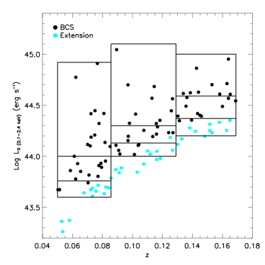
Figure 5: eBCS clusters. Cluster binning in equally populated z and $L_{\rm X}$ bins. Black full dots represent BCS clusters (Ebeling et al., 1998) while cyan ones stand for extension clusters (Ebeling et al., 2000)

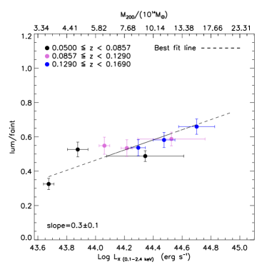
Figure 6: eBCS clusters. Luminous to faint ratios as function of $\log(L_{\rm X})$. The values reported in the plot are the average values of the lum/faint ratios and of $\log(L_{\rm X})$ obtained in the z and $L_{\rm X}$ bins shown in Fig. 5. A mass scale is also shown, inferred using the $M_{\rm 200}-L_{\rm X}$ relation of Popesso et al. (2005). The best-fitting line (dashed line), whose slope is displayed at the lower left corner of this plot, is reported. The error on the slope is evaluated through a jackknife technique.

The biweight fit performed on the stacked colour-magnitude diagrams of the cluster samples studied in this work, produces estimates of the CMR slope consistent among themselves within $2\sigma$. The values shown are about $-0.034$, in accordance with other studies based on observations (e.g. Stott et al., 2009). Despite this, as reported in similar studies, a discrepancy is seen when the CMR slopes are compared with the findings inferred through theoretical models. In fact, our values are not consistent with any of those obtained through the model by T. Kodama (see Kodama & Arimoto, 1997 for the description of the model) in the SDSS bands for several galaxy formation redshifts. This is probably due to the fact that our slope values are obtained for stacked CMRs, containing several and possibly diverse clusters, while this model is calibrated to the CMR of the Coma cluster.

$\mathbf{r}_{{}_{\rm AB,C}}$	$\mathbf{r}_{{}_{\rm AC,B}}$	$\mathbf{r}_{{}_{\rm BC,A}}$
0.02 ($\sim 45\%$)	0.15 ($\sim 2.5\%$)	0.66 ($<0.05\%$)

Table 3: Results of partial Spearman rank correlation tests for eBCS cluster sample. The tests are performed for lum/faint ratios (A), $\log(L_{X})$ (B) and z (C). In brackets is reported the probability of obtaining a partial rank correlation coefficient with absolute value as large as, for instance, $|r_{{}_{\rm AB}}|$, or larger, under the null hypothesis that the correlation between A and B results solely from correlations between A and C and between B and C.

7 Discussion

Tab. 1 shows that the lum/faint ratios between optical and X-ray clusters vary by as much as $30$ per cent within a single redshift bin, which, on its own, goes some way to explain the variation in the literature values at low redshift. The HB sample gives the lowest lum/faint ratio of the three samples at all redshifts, which is easily explained as the selection algorithm for this sample is based on the cluster density profile fit, in contrast to the B and eBCS, which are based on the presence of bright red galaxies and BCGs; the close correlation between cluster X-ray brightness, used to select the eBCS, and BCG magnitude has been known for some time (e.g. Edge, 1991; Collins & Mann, 1998).

The degree of evolution in the lum/faint ratio at high redshift is still somewhat confused. Measurement of this ratio has now been made in the highest redshift X-ray cluster known (J2215-1735) at $z=1.46$ (Hilton et al., 2009). However, in contrast to the Andreon clusters at $z>1$ previously discussed, J2215 has a lum/faint ratio of $2.2\pm 0.9$ when transformed onto the De Lucia system, a value consistent with the prediction of $\simeq 1.3$ based on a simple extrapolation of our best-fitting line in Fig. 4.

The evidence for evolution in the lum/faint ratio seen in Fig. 4 results from the deficit of faint galaxies on the red sequence in comparison to clusters observed at lower redshifts. Taken at face value, this is consistent with higher mass galaxies ending their star formation earlier than in their low mass counterparts; a process dubbed as downsizing (Cowie et al., 1996). However the question still remains as to the process by which the CMR becomes populated with RSGs and in particular whether the dominant mechanism is through merging or the stripping of spiral and irregular galaxies transforming them into passive S0s; an idea that is supported by the decrease in S0 galaxies along with the increasing fraction of spiral and irregular galaxies with redshift (Dressler et al., 1997; Smith et al., 2005; Postman et al., 2005).

Our partial Spearman results offer at least one possible clue; the lack of an underlying correlation between lum/faint ratio and $L_{\rm x}$ over our redshift range suggests that at least the late-time build up of the CMR is not related to processes associated with the hot intra cluster medium, such as ram pressure stripping or other mechanisms that depend on cluster mass, like tidal stripping or harassment (Wake et al., 2005; Mei et al., 2009; Stott et al., 2007); however the large variation in the lum/faint ratio for massive clusters at $z\geq 1$ previously mentioned, indicates that this issue is far from settled. Furthermore, our partial Spearman results highlight the importance of appropriate statistical analyses in determining the significance of possible correlation trends, particularly when faced with flux-limited samples.

Turning to the possible role of mergers, since the fraction of massive early-type galaxies in clusters has been shown to remain consistently high out to $z=0.8$, the evolution seen in magnitude-limited samples may be dominated by fainter (sub-$M^{\ast}$ in the stellar mass) galaxies undergoing merging (van der Wel et al., 2007; Holden et al., 2007). An important recent development possibly related to this is the discovery of early-type massive compact ($\simeq 1$kpc) galaxies at $z\simeq 2$ (e.g. Trujillo et al., 2006; Toft et al., 2007; van Dokkum et al., 2009). The dearth of such objects in local samples (Taylor et al., 2009) implies that these galaxies must undergo a rapid size evolution, growing by a factor $\simeq 4-5$ since $z=2-3$. Among the models that have been proposed the currently favoured mechanism driving this growth is also through minor merging with sub-$M^{\ast}$ galaxies (e.g. Naab et al., 2009). Although most attention has focused on high redshift compact galaxies in the field, if the merging explanation is correct it should also apply to ellipticals in clusters. It therefore remains to be seen if a single sub-$M^{\ast}$ population in clusters can explain both the build up onto the CMR and the rapid size evolution of ellipticals. On the other hand, it needs to be stressed that the local dearth of these early-type massive compact galaxies and their rapid size evolution are still a controversial issue. In fact, Valentinuzzi et al. (2009) claimed that such objects might exist also locally in clusters, while Hopkins et al. (2010) suggested different mechanisms driving a more modest size evolution. Finally, but not less important, Muzzin et al. (2009) pointed out the estimated masses of these objects may be extremely uncertain.

We plan future investigations of the CMR using statistical samples of clusters over a wide redshift range from the serendipitous XCS cluster sample based on $XMM-Newton$ (Sahlén et al., 2009; Hilton et al., 2009) whose flux limit ($3.5\times 10^{-13}\ {\rm erg\ cm^{-2}\ s^{-1}}$) is an order of magnitude lower than the eBCS sample used here, which will enable trends with $L_{\rm X}$ to be reliably determined over a broad redshift range and allow us to investigate the CMR evolution in more detail in the redshift range $z=1-2$.

8 Conclusions

We study the lum/faint ratio of RSGs for a large sample of optically (266) and X-ray (112) selected galaxy clusters in the sparsely covered regime ($0.05\leq z<0.19$) using data from the SDSS DR6 to investigate how this ratio varies between different cluster samples (optical and X-ray) and to investigate possible trends with cluster mass and redshift, reported by other authors.

• Independent of the method used, we find values of the lum/faint ratio consistent with those found by De Lucia et al. (2007) for SDSS clusters, and a correlation with redshift [$\log({\rm lum/faint})=(1.2\pm 0.1)\log(1+z)$], confirming a continuous trend in downsizing to low redshift.
  

• From a partial Spearman rank correlation test, we find no trend of lum/faint ratio with $L_{\rm X}$ when correlations between $L_{\rm X}$ and z and between lum/faint ratio and z are removed, in agreement with the suggestion of Gilbank & Balogh (2008) and Andreon (2008). This may be due to the narrow cluster mass range investigated.
  

• The CMR slopes are $\sim-0.034$ for all the samples and consistent within $2\sigma$ of each other. These are similar to the values obtained in similar observational studies using similar rest-frame colours (e.g. Stott et al., 2009); however they are inconsistent with the ones inferred through the theoretical model by Kodama & Arimoto (1997). This may be due to the fact that this model is calibrated to the CMR of the Coma cluster, while we obtain slopes for stacked CMRs, containing several and possibly diverse clusters.

Acknowledgments

The authors thank the referee for his/her valid comments.
We thank Dr. G. De Lucia, for having kindly provided her data. We also thank Dr. T. Kodama for providing access to his models.
The authors acknowledge Dr. E. De Filippis for having provided the list of the control fields for the background subtraction and thank Dr. M. Hilton for helpful conversations.
DC expresses his gratitude to Dr. E. De Filippis, Dr. M. Paolillo, Prof. G. Longo and Dr. R. D’Abrusco, of the Department of Physical Sciences at the University of Napoli Federico II, for the valuable discussions. DC also thanks Dr. Cristiano Porciani for the useful suggestions.
Funding for the Sloan Digital Sky Survey (SDSS) and SDSS-II has been provided by the Alfred P. Sloan Foundation, the Participating Institutions, the National Science Foundation, the U.S. Department of Energy, the National Aeronautics and Space Administration, the Japanese Monbukagakusho, the Max Planck Society and the Higher Education Funding Council for England. The SDSS Web site is http://www.sdss.org/.

References

- Andreon (2008) Andreon S., 2008, MNRAS, 386, 1045
- Bahcall et al. (2003) Bahcall N. A., et al., 2003, ApJS, 148, 243
- Barkhouse et al. (2007) Barkhouse W. A., Yee H. K. C., López-Cruz O., 2007, ApJ, 671, 1471
- Barkhouse et al. (2009) Barkhouse W. A., Yee H. K. C., López-Cruz O., 2009, ApJ, 703, 2024
- Beers et al. (1990) Beers T. C., Flynn K., Gebhardt K., 1990, AJ, 100, 32
- Blanton & Roweis (2007) Blanton M. R., Roweis S., 2007, AJ, 133, 734
- Capozzi et al. (2009) Capozzi D., De Filippis E., Paolillo M., D’Abrusco R., Longo G., 2009, MNRAS, 396, 900
- Collins & Mann (1998) Collins C. A., Mann R. G., 1998, MNRAS, 297, 128
- Cowie et al. (1996) Cowie L. L., Songaila A., Hu E. M., Cohen J. G., 1996, AJ, 112, 839
- Cross et al. (2004) Cross N. J. G., Driver S. P., Liske J., Lemon D. J., Peacock J. A., Cole S., Norberg P., Sutherland W. J., 2004, MNRAS, 349, 576
- De Filippis et al. (2009, in preparation) De Filippis E., et al., 2009, in preparation
- De Lucia et al. (2004) De Lucia G., et al., 2004, ApJ Let., 610, L77
- De Lucia et al. (2007) De Lucia G., et al., 2007, MNRAS, 374, 809
- Dressler et al. (1997) Dressler A., et al., 1997, ApJ, 490, 577
- Ebeling et al. (2000) Ebeling H., Edge A. C., Allen S. W., Crawford C. S., Fabian A. C., Huchra J. P., 2000, MNRAS, 318, 333
- Ebeling et al. (1998) Ebeling H., Edge A. C., Bohringer H., Allen S. W., Crawford C. S., Fabian A. C., Voges W., Huchra J. P., 1998, MNRAS, 301, 881
- Edge (1991) Edge A. C., 1991, MNRAS, 250, 103
- Fukugita et al. (1996) Fukugita M., Ichikawa T., Gunn J. E., Doi M., Shimasaku K., Schneider D. P., 1996, AJ, 111, 1748
- Fukugita et al. (1995) Fukugita M., Shimasaku K., Ichikawa T., 1995, PASP, 107, 945
- Gilbank & Balogh (2008) Gilbank D. G., Balogh M. L., 2008, MNRAS, 385, L116
- Gilbank et al. (2008) Gilbank D. G., Yee H. K. C., Ellingson E., Gladders M. D., Loh Y.-S., Barrientos L. F., Barkhouse W. A., 2008, ApJ, 673, 742
- Gladders et al. (1998) Gladders M. D., Lopez-Cruz O., Yee H. K. C., Kodama T., 1998, ApJ, 501, 571
- Hansen et al. (2009) Hansen S. M., Sheldon E. S., Wechsler R. H., Koester B. P., 2009, ApJ, 699, 1333
- Hilton et al. (2009) Hilton M., et al., 2009, ApJ, 697, 436
- Holden et al. (2007) Holden B. P., et al., 2007, ApJ, 670, 190
- Hopkins et al. (2010) Hopkins P. F., Bundy K., Hernquist L., Wuyts S., Cox T. J., 2010, MNRAS, 401, 1099
- Kauffmann & Charlot (1998) Kauffmann G., Charlot S., 1998, MNRAS, 294, 705
- Kim et al. (2002) Kim R. S. J., et al., 2002, AJ, 123, 20
- Kodama & Arimoto (1997) Kodama T., Arimoto N., 1997, A&A, 320, 41
- Koester et al. (2007) Koester B. P., et al., 2007, ApJ, 660, 221
- Koyama et al. (2007) Koyama Y., Kodama T., Tanaka M., Shimasaku K., Okamura S., 2007, MNRAS, 382, 1719
- Lu et al. (2009) Lu T., Gilbank D. G., Balogh M. L., Bognat A., 2009, MNRAS, pp 1293–+
- Mei et al. (2009) Mei S., et al., 2009, ApJ, 690, 42
- Muzzin et al. (2009) Muzzin A., van Dokkum P., Franx M., Marchesini D., Kriek M., Labbé I., 2009, ApJ Let., 706, L188
- Naab et al. (2009) Naab T., Johansson P. H., Ostriker J. P., 2009, ApJ Let., 699, L178
- Poggianti (1997) Poggianti B. M., 1997, A&AS, 122, 399
- Popesso et al. (2005) Popesso P., Biviano A., Böhringer H., Romaniello M., Voges W., 2005, A&A, 433, 431
- Postman et al. (2005) Postman M., et al., 2005, ApJ, 623, 721
- Sahlén et al. (2009) Sahlén M., et al., 2009, MNRAS, 397, 577
- Schechter (1976) Schechter P., 1976, ApJ, 203, 297
- Smith et al. (2005) Smith G. P., Treu T., Ellis R. S., Moran S. M., Dressler A., 2005, ApJ, 620, 78
- Stott et al. (2009) Stott J. P., Pimbblet K. A., Edge A. C., Smith G. P., Wardlow J. L., 2009, MNRAS, pp 304–+
- Stott et al. (2007) Stott J. P., Smail I., Edge A. C., Ebeling H., Smith G. P., Kneib J.-P., Pimbblet K. A., 2007, ApJ, 661, 95
- Swinbank et al. (2007) Swinbank A. M., et al., 2007, MNRAS, 379, 1343
- Tanaka et al. (2005) Tanaka M., Kodama T., Arimoto N., Okamura S., Umetsu K., Shimasaku K., Tanaka I., Yamada T., 2005, MNRAS, 362, 268
- Taylor et al. (2009) Taylor E. N., Franx M., Glazebrook K., Brinchmann J., van der Wel A., van Dokkum P. G., 2009, ArXiv e-prints
- Toft et al. (2007) Toft S., et al., 2007, ApJ, 671, 285
- Trujillo et al. (2006) Trujillo I., et al., 2006, ApJ, 650, 18
- Valentinuzzi et al. (2009) Valentinuzzi T., et al., 2009, ArXiv e-prints
- van der Wel et al. (2007) van der Wel A., et al., 2007, ApJ, 670, 206
- van Dokkum et al. (2009) van Dokkum P. G., Kriek M., Franx M., 2009, Nature, 460, 717
- Visvanathan & Sandage (1977) Visvanathan N., Sandage A., 1977, ApJ, 216, 214
- Wake et al. (2005) Wake D. A., Collins C. A., Nichol R. C., Jones L. R., Burke D. J., 2005, ApJ, 627, 186
- Yang et al. (2007) Yang X., Mo H. J., van den Bosch F. C., Pasquali A., Li C., Barden M., 2007, ApJ, 671, 153