Nonlinear force-free modelling: influence of inaccuracies in the measured magnetic vector.

Abstract

Context. Solar magnetic fields are regularly extrapolated into the corona starting from photospheric magnetic measurements that can suffer from significant uncertainties.

Aims. Here we study how inaccuracies introduced into the maps of the photospheric magnetic vector from the inversion of ideal and noisy Stokes parameters influence the extrapolation of nonlinear force-free magnetic fields.

Methods. We compute nonlinear force-free magnetic fields based on simulated vector magnetograms, which have been produced by the inversion of Stokes profiles, computed from a 3-D radiation MHD simulation snapshot. These extrapolations are compared with extrapolations starting directly from the field in the MHD simulations, which is our reference. We investigate how line formation and instrumental effects such as noise, limited spatial resolution and the effect of employing a filter instrument influence the resulting magnetic field structure. The comparison is done qualitatively by visual inspection of the magnetic field distribution and quantitatively by different metrics.

Results. The reconstructed field is most accurate if ideal Stokes data are inverted and becomes less accurate if instrumental effects and noise are included. The results demonstrate that the non-linear force-free field extrapolation method tested here is relatively insensitive to the effects of noise in measured polarization spectra at levels consistent with present-day instruments.

Conclusions. Our results show that we can reconstruct the coronal magnetic field as a nonlinear force-free field from realistic photospheric measurements with an accuracy of a few percent, at least in the absence of sunspots.

1 Introduction

Except for a few individual cases, e.g., in newly developed active regions (Solanki et al., 2003), we cannot measure the full magnetic vector in the solar corona at high resolution directly and we have to rely on extrapolations from photospheric measurements. Wiegelmann et al. (2005b) compared the direct magnetic field measurements by Solanki et al. (2003) with extrapolations from the photosphere. This work revealed the importance of field aligned electric currents for an accurate magnetic field reconstruction and the need for photospheric vector magnetograms as boundary data. The photospheric data suffer from a number of inadequacies, however, whose influence on the quality of the extrapolations needs to be studied in detail. Firstly, the magnetic field in the photosphere is far from being force-free, (see, e.g., Metcalf et al., 1995), which leads to significant errors if used directly for a force-free magnetic field extrapolation (see Metcalf et al., 2008, for details). These can, however, be greatly reduced by appropriate preprocessing (Wiegelmann et al., 2006b). Another well known problem is that the noise level of the magnetic field transverse to the line of sight is typically more than one order of magnitude higher than for the longitudinal component deduced from the Stokes parameters of Zeeman split spectral lines. An additional complication arises for vector magnetic field measurements made far away from the disk center, where the vertical and line-of-sight field are far apart (see Gary & Hagyard, 1990, for details). In this case one has to use also the transverse field to derive the vertical field. Venkatakrishnan & Gary (1989) showed that the increased noise by using the transverse field is tolerable for heliocentric distances of less than $50^{\circ}$. For our investigations we assume that the observations are made close to the disk center, where the vertical magnetic field is almost identical with the line-of-sight field and the horizontal component is almost identical with the transverse field. Consequently our results are not directly applicable to regions observed for heliocentric distances of larger than about $50^{\circ}$, where the noise in the transverse field influences significantly the accuracy of the vertical field. Furthermore, high resolution vector magnetographs such as Hinode/SOT have a limited field of view, which often does not allow deriving the horizontal magnetic field in an entire active region. The influence of these effects on the accuracy of non-linear force-free extrapolations have recently been investigated in DeRosa et al. (2009). Less often considered are effects introduced by the fact that the extraction of the field from the Stokes parameters is intrinsically uncertain. E.g., the measured Stokes profiles are formed in a highly dynamic atmosphere with a complex thermal and magnetic structure, while the normally applied inversion methods impose rather restrictive assumptions (e.g. Milne-Eddington atmosphere, Auer et al., 1977). In addition, due to the spatially fluctuating height of formation of the lines, the obtained magnetic vector refers to different heights in the atmosphere at different locations. For extrapolation methods one has to assume a single, often planar, height as the boundary condition. Finally, instrumental limitations impose restrictions, such as limited spatial and spectral resolution, spectral sampling (in particular for filter instruments) and noise.

Here we investigate how the extrapolated coronal magnetic field is influenced by noise and other instrumental artifacts (spatial resolution, limited spectral sampling), as well as the general limitations of the inversion of the measured Stokes profiles. To do so we use the results of 3D radiation MHD simulations. We compute synthetic lines from the data cubes of the relevant physical quantities, add noise and apply the influence of typical instrument parameters. Finally we invert these artificial measurements to derive synthetic vector magnetograms, which are then used as boundary conditions for a nonlinear force-free magnetic field extrapolation. We compare the reconstruction from ideal data, taken directly from the MHD simulations, with extrapolations starting from data containing instrumental effects and noise of different levels of severity. Our aim is to investigate how different instrumental effects and noise influence a nonlinear force-free magnetic field extrapolation. Besides testing generally the influence of reduced spatial resolution of the photospheric magnetic field data, we also consider to what extend the properties of specific high resolution space instruments affect the quality of the extrapolations. The two instruments we consider are the Spectro-Polarimeter (SP) on the Solar Optical Telescope (SOT) on the Hinode spacecraft (Shimizu, 2004; Tsuneta et al., 2008) and the Polarimetric and Helioseismic Imager (PHI) to fly on the Solar Orbiter mission. Instruments with lower spatial resolution, such as the Helioseismic Magnetic Imager (HMI) were not considered, since the number of pixels across the MHD simulation box are then rather small, making a meaningful test more improbable.

2 Method

2.1 Setup of the test case

We start with 3-D radiation MHD simulations resulting from the MURAM code (see Vögler et al., 2005, for details). The particular snapshot considered here has been taken from a bipolar run and harbours equal amounts of magnetic flux of both polarities. The configuration has an average field strength of $150$ G at the spatially averaged continuum optical depth $\langle\tau_{5000}\rangle=1$ at $5000$ Å. The horizontal dimensions of the simulation domain are $6\times 6{\rm Mm}$ and $1.4{\rm Mm}$ in the vertical direction. The original resolution is $20{\rm km}$ in the horizontal directions and $14{\rm km}$ in the vertical direction. Similar snapshots have also been used by Khomenko et al. (2005b) for the investigation of magnetoconvection of mixed-polarity quiet-Sun regions and compared with measured Stokes profiles by Khomenko et al. (2005a).

Due to the limited height-range of the MHD simulation we first extrapolate the field from the magnetic vector obtained from the simulations at a fixed geometric height (see Fig. 1). This height, $Z_{\rm ref}$, must be chosen with care since the extrapolation starting from the magnetic field vector at $Z_{\rm ref}$ is employed as a reference against which all others are compared. In order to avoid introducing a bias it must correspond to a suitably weighted average height of formation of the spectral line used for inversion, e.g. Fe I $6173.3$ Å. Since different regions in the MHD-simulation may have different formation height ranges, we have chosen a criterion to select the reference height which is obtained by finding the highest correlation between the magnetic field strength taken directly from the MHD simulation and from inversion of the Stokes profiles obtained under ideal conditions (very high spectral and spatial resolutions and no noise).

This extrapolation is used as reference, with which other extrapolations are compared. These later ones use magnetic vector maps that are obtained from the inversion of synthetic Stokes profiles.

Two spectral lines are considered, the very widely used Fe I $6302.5$ Å (Landé factor $g=2.5$) line, employed by the Advanced Solar Polarimeter and the spectropolarimeter on the Hinode spacecraft and the Fe I $6173.3$ Å ($g=2.5$), which has been selected for the Helioseismic and Magnetic Imager (HMI) on the Solar Dynamics Observatory (SDO) and for the Polarimetric and Helioseismic Imager on the Solar Orbiter mission (SO/PHI). For both $Z_{\rm ref}$ was found to lie approximately at $150$ km above $\langle\tau_{5000}\rangle=1$.

Next, using the STOPRO code (Solanki, 1987; Frutiger et al., 2000), we compute the Stokes parameters of these widely used spectral lines. We restrict ourselves to considering the situation at solar disk center. These synthetic data are then either directly inverted, or after degrading the data by introducing noise, lowering the spatial and/or the spectral resolution, etc. A list of all the considered cases is presented in Table 1 and discussed in Sect. 3. The inversion is carried out for each spectral line individually. The inverted magnetic field vector is then taken as the starting point for a non-linear force-free extrapolation.

For comparison we also compute a potential field from the results of the MHD-simulations at $Z_{\rm ref}$, which requires only the vertical component of the photospheric magnetic field. In addition, we compute nonlinear force-free extrapolations with the horizontal spatial resolution reduced by a factor of two and four, respectively, compared to the original MHD model.

2.2 Description of the inversion code

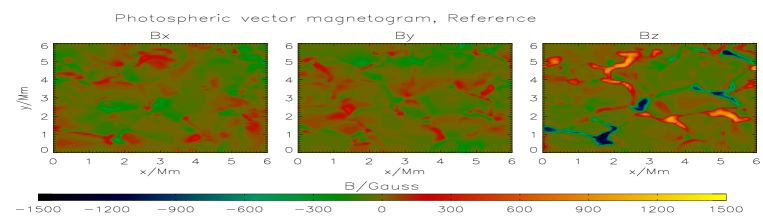
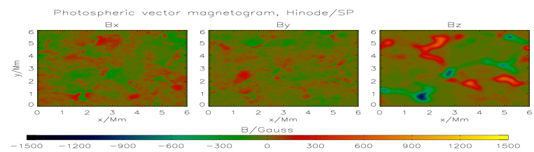
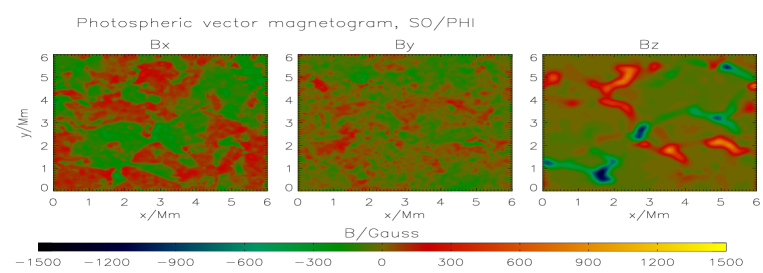
Figure 1: $B_{x},B_{y},B_{z}$ maps at a fixed reference height $Z_{\rm ref}$ approximately 150 km above the average $<\tau_{5000}>=1$. The top panel contains the original maps from the MHD data, which are used as a reference. The second panel shows the results of an inversion with Filter and noise. The third and bottom panel correspond to simulated inversions from Hinode/SP and SO/PHI, respectively. For a quantitative comparison see Table 1.

The inversion code HeLIx developed by Lagg et al. (2004) is based on fitting the observed Stokes profiles with synthetic ones obtained from an analytic solution of the Unno-Rachkovsky equations (Unno, 1956; Rachkowsky, 1967) in a Milne-Eddington atmosphere (see e.g. Landi degl’Innocenti, 1992). These synthetic profiles are functions of the magnetic field strength $|B|$, its inclination and azimuth (with respect to the line of sight), the vertical velocity, the Doppler width, the damping constant, the ratio of the line center to the continuum opacity, and the slope of the source function with respect to optical depth. We assume the filling factor to be unity. Any possible magnetic fine structure within one pixel consisting of a field-free and a magnetic area is smeared out, and the inversion returns the magnetic field vector averaged over the considered pixel. Since the extrapolations are performed on the same pixel scale as the inversions, the extrapolations must be fed with the pixel-averaged magnetic field vector. Setting the filling factor to unity already during the inversion process enhances its robustness and reliability. The atmospheric parameters that ensure the minimum of the merit function are obtained using a very reliable genetic algorithm (Charbonneau, 1995). The genetic algorithm has been extensively tested with synthetic spectra from MHD simulations and the result compared with response-function-averaged physical parameters (e.g. magnetic field strength, inclination, azimuth, line-of-sight velocity). The results of the test indicate that the genetic algorithm retrieves the global minimum of the merit function with high reliability. The parameter sets are chosen to, e.g., mimic the effects of the Hinode/SOT and the future SO/PHI instruments, respectively.

2.3 Hinode SOT Spectro-polarimeter

The spectropolarimeter (SP; Lites et al., 2007) is part of the focal-plane package of the $50cm$ Solar Optical Telescope (SOT) onboard the Hinode spacecraft. It observes the line pair Fe I $6302.5$ and $6301.5$ Å. Here we restrict ourselves to $6302.5$ Å. The spatial resolution at the diffraction limit of the telescope’s primary mirror is about 0.32” at $6302.5$ Å, which corresponds to 230 km on the Sun. The size of a detector pixel corresponds to approximately 110 km on the Sun in the spatial direction. The spectral resolution is $30$ mÅ and the spectral sampling is $21$ mÅ. We used Gaussians for spectral and spatial smearing. The noise has been added to the Stokes profiles as photon noise $F\times 1/\sqrt{I_{c}}$, where $F$ is a white noise with a Gaussian distribution and $I_{c}$ is the continuum intensity. The chosen standard deviation of $F$ was $10^{-3}$, which corresponds to the typical noise level for modern spectropolarimetric observations (e.g. Hinode/SP data). Noise is included in a similar way wherever we mention that noise has been added to the data. More subtle instrumental effects such as scattered light, or a slight defocus (e.g. Danilovic et al., 2008), are not considered.

2.4 SO/PHI magnetograph

The Solar Orbiter Polarimetric and Helioseismic Imager (SO/PHI), a vector magnetograph, will be one of the main instruments on the ESA-NASA Solar Orbiter mission. Of its two telescopes, the High Resolution Telescope (HRT) is of primary importance for the present investigation (due to the small horizontal extent of the MHD simulations). The spectral line chosen for SO/PHI, Fe I $6173.3$ Å, combines high Zeeman sensitivity with spectral purity, needed for simultaneous vector magnetic field and helioseismology studies. We describe the point spread function (PSF) by a Gaussian with FWHM$=150$ km. The obtained arrays of Stokes parameters are rebinned to a spatial pixel size of $80$km. We then convolve the Stokes profiles in the spectral dimension with a Fabry-Pérot type filter with ${\rm FWHM}=100$ mÅ. Since SO/PHI will be a filtergraphic instrument, we decrease the number of spectral samples per line by taking 5 positions in the line and one in the continuum at the positions (from line center at rest): -0.3Å, -0.15Å, -0.075 Å, 0 Å, +0.075 Å, +0.15 Å. At that stage we add noise and perform the inversion of the Stokes profiles.

2.5 Extrapolation of the vector magnetogram into the atmosphere

To compute a 3D-nonlinear force-free magnetic field from the result of the HeLIx inversion code we carry out the following steps:

• If needed, transform $B,\,\theta$ and $\phi$, which are output from the inversion code, to $B_{x},\,B_{y},\,B_{z}$ on the photosphere, which requires a resolution of the $180^{\circ}$ ambiguity in $\phi$. (See section 2.5.1.)

• Preprocess the vector magnetogram ($B_{x},\,B_{y},\,B_{z}$), assuming that it refers to the same geometric height at every spatial pixel. (See Sect. 2.6.1.)

• Compute a nonlinear force-free coronal magnetic field from the preprocessed vector magnetogram. (See Sect. 2.6.2.)

• Compare the result with the reference field.

We explain these steps in the following.

2.5.1 Removal of the $180^{\circ}$ ambiguity.

For the purpose of the present investigation we have chosen to remove the $180^{o}$ ambiguity by minimizing the angle to the exact solution. This possibility does, of course, not exist for real data and other methods for the ambiguity inversion would need to be tried. The performance of different ambiguity removal techniques has been studied with synthetic data by Metcalf et al. (2006). They found that the best available technique managed to get $100\%$ of the points correctly. Recently the influence of noise and spatial resolution on the quality of the different ambiguity removal techniques has been investigated by Leka et al. (2009). We have therefore not considered specific ambiguity removal techniques. An investigation of their efficiency and influence is outside the scope of this paper.

Table 1: Influence on the photospheric field for different cases.

Case studied	$C_{Bx}$	$C_{By}$	$C_{Bz}$	$C_{\rm vec}$	$<|J_{z}|>$	$<|B_{z}|>$
Reference	$1$	$1$	$1$	$1$	$0.059$	$103.5$
Inversion of synthetic profiles (tests)
Full resolution, no noise and full profiles
$6302.5$ Å	$0.89$	$0.88$	$0.97$	$0.96$	$0.065$	$96.7$
$6173.3$ Å	$0.89$	$0.88$	$0.97$	$0.96$	$0.065$	$95.9$
Full resolution, with noise and full profiles
$6302.5$ Å	$0.87$	$0.86$	$0.97$	$0.95$	$0.086$	$97.6$
$6173.3$ Å	$0.88$	$0.88$	$0.97$	$0.95$	$0.070$	$96.5$
Full resolution, with Filters $(5+1\lambda)$ values
$6173.3$ Å no noise	$0.86$	$0.85$	$0.97$	$0.95$	$0.084$	$96.0$
$6173.3$ Å w. noise	$0.72$	$0.70$	$0.97$	$0.90$	$0.213$	$96.7$
Hinode/SP
no noise	$0.80$	$0.77$	$0.84$	$0.82$	$0.047$	$79.4$
$10^{-3}$ noise	$0.76$	$0.71$	$0.84$	$0.81$	$0.067$	$80.7$
SO/PHI
no noise	$0.79$	$0.68$	$0.85$	$0.82$	$0.078$	$84.5$
$10^{-3}$ noise	$0.67$	$0.53$	$0.85$	$0.73$	$0.184$	$85.2$

2.6 Effects in the photosphere

In Table 1 and in figure 1we investigate how the different instrument effects and noise influence the vector field in the photosphere. The first line corresponds to the MHD reference field. The field has an average electric current density of $\langle|J_{z}|\rangle=0.059A/m^{2}$ and a vertical magnetic field strength of $\langle|B_{z}|\rangle=103.5G$. Positive and negative values of these quantities are balanced. In the table we compute the correlation relative to this reference case for the horizontal fields $C_{Bx},\,C_{By}$, the vertical field $C_{Bz}$ and the 2D-vector correlation in the photosphere $C_{\rm vec}$ and provide the average absolute values $\langle|B_{z}|\rangle$ and $\langle|J_{z}|\rangle$. For all full spatial resolution cases (upper part of the table) the correlation for the different cases is $0.97$ for the vertical magnetic field strength and the average field strength is underestimated by a few percent. Noise and instrument effects seem to have a relative small effect on the vertical field. The effect of a reduced resolution (lower part of the figure, Hinode/SP and SO/PHI cases) on the horizontal photospheric magnetic fields $B_{x},\,B_{y}$ and the derived vertical current density $J_{z}$ is significantly higher. While for full profiles the correlation in the horizontal fields is in the range of $0.85-0.88$, the combined effect of filter and noise reduces the correlation to only $0.70$ and spurious, non-physical electric currents, which results in an overestimation of $J_{z}$ by a factor of about $3$.

2.6.1 Preprocessing

The magnetic field in the photosphere is not necessarily force-free (because of the finite $\beta$ plasma in the photosphere, see Gary, 2001) and the horizontal components ($B_{x}$ and $B_{y}$) of current vector magnetographs have large uncertainties. Aly (1989) defined a number of integral relations to evaluate if a measured photospheric vector magnetogram is consistent with the assumption of a force-free field. These integral relations (numerator in Eq. 1) have been used to define a dimensionless parameter $\epsilon_{\mbox{force}}$ as

$$\frac{|\int_{S}B_{x}B_{z}\;dx\,dy|+|\int_{S}B_{y}B_{z}\;dx\,dy|+|\int_{S}(B_{x}^{2}+B_{y}^{2})-B_{z}^{2}\;dx\,dy|}{\int_{S}(B_{x}^{2}+B_{y}^{2}+B_{z}^{2})\;dx\,dy}$$ (1)

and force-free extrapolation codes require $\epsilon_{\mbox{force}}\ll 1$ on the boundary. (One gets $\epsilon_{\mbox{force}}=0$ if the integral relations are fulfilled exactly).

For the synthetic magnetograms investigated in table 1 we find $\epsilon_{\mbox{force}}=0.57\pm 0.19$ in the photosphere. Wiegelmann et al. (2006b) developed a preprocessing procedure to drive the observed non force-free data towards boundary conditions suitable for a force-free extrapolation. As a result of the preprocessing we get a boundary-data set which is consistent with the assumption of a force-free magnetic field. After applying the preprocessing-routine we get force-free consistent boundary conditions with $\epsilon_{\mbox{force}}=(2.6\pm 0.2)\cdot 10^{-4}$. The preprocessing affects mainly the horizontal magnetic field components. The correlation of original and preprocessed field for the investigated cases is $C_{Bz}=0.99\pm 0.006$ for the vertical component $B_{z}$. For the horizontal components we find a correlation of $C_{Bx}=0.91\pm 0.05$ and $C_{By}=0.90\pm 0.05$, respectively.

2.6.2 Extrapolation of nonlinear force-free fields.

Force-free coronal magnetic fields have to obey the equations

$$(\nabla\times{\bf B})\times{\bf B} = {\bf 0},$$ (2)

$$\nabla\cdot{\bf B} = 0.$$ (3)

We define the functional

$$L=\int_{V}\;w\;\left[\;B^{-2}\,|(\nabla\times{\bf B})\times{\bf B}|^{2}+\;|\nabla\cdot{\bf B}|^{2}\right]\;d^{3}x,$$ (4)

where $w$ is a weighting function. It is obvious that (for $w>0$) the force-free equations (2-3) are fulfilled when L is equal to zero (Wheatland et al., 2000). We minimize the functional (4) numerically as explained in detail by Wiegelmann (2004). The program is written in C and has been parallelized with OpenMP. Wiegelmann & Neukirch (2003) and Schrijver et al. (2006) tested the program with exact nonlinear force-free equilibria of Low & Lou (1990), while Wiegelmann et al. (2006a) tested it with another exact equilibrium developed by Titov & Démoulin (1999). The code has been applied to vector magnetograph data from the German Vacuum Tower Telescope (VTT) by Wiegelmann et al. (2005a, b) and to data from the Solar Flare Telescope (SFT) by Wiegelmann et al. (2006b). Here we use an updated version of the optimization approach, including a multi-scale approach which has been described and tested by Metcalf et al. (2008) and applied to Hinode data by (Schrijver et al., 2008).

Table 2: Various figures of merit of the 3D reconstruction for different cases.

Case studied	$C_{\rm vec}$	$\epsilon$	$C_{\rm 100km}$	$C_{\rm 400km}$	$C_{\rm 800km}$
Reference	$1$	$1$	$1$	$1$	$1$
Potential	$0.68$	$0.62$	$0.72$	$0.84$	$0.97$
MHD cases with reduced resolution
Pixel Size 40km	$0.99$	$0.93$	$0.99$	$1.00$	$1.00$
Pixel Size 80km	$0.93$	$0.79$	$0.94$	$0.96$	$0.99$
Inversion of synthetic profiles (tests)
Full resolution, no noise and full profiles
$6302.5$ Å	$0.92$	$1.06$	$0.93$	$0.98$	$1.00$
$6173.3$ Å	$0.93$	$0.99$	$0.93$	$0.98$	$0.99$
Full resolution, with noise and full profiles
$6302.5$ Å	$0.93$	$1.04$	$0.93$	$0.98$	$1.00$
$6173.3$ Å	$0.93$	$1.05$	$0.93$	$0.98$	$0.99$
Full resolution, with Filters $(5+1\lambda)$ values
$6173.3$ Å no noise	$0.92$	$1.06$	$0.92$	$0.98$	$0.99$
$6173.3$ Å w. noise	$0.91$	$1.10$	$0.89$	$0.97$	$0.99$
Hinode/SP
no noise	$0.85$	$0.66$	$0.85$	$0.96$	$0.99$
$10^{-3}$ noise	$0.84$	$0.62$	$0.84$	$0.95$	$0.99$
SO/PHI
no noise	$0.84$	$0.75$	$0.85$	$0.96$	$0.99$
$10^{-3}$ noise	$0.81$	$0.76$	$0.78$	$0.90$	$0.98$

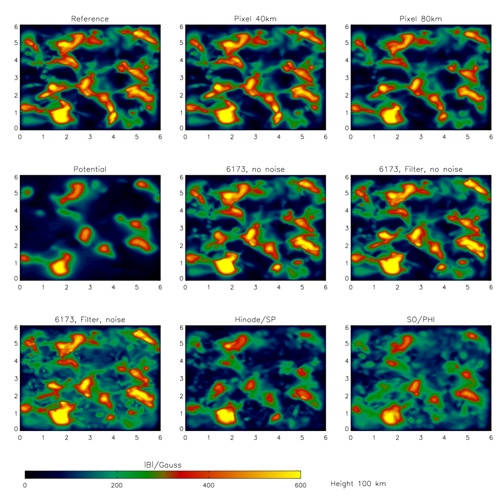
Figure 2: $|{\bf B}|$ for the reference field and extrapolated from inversion of synthetic profiles. The plots display $|{\bf B}|$ at a height of $100km$ above the reference height (See Sect. 2.1 for a definition). The figure shows, from top-left to bottom-right, the ideal reference solution (indicated as Reference); extrapolations starting from the MHD output after reducing its spatial resolution (Pixel 40km and Pixel 80km, respectively); a potential field reconstruction (Potential); a reconstruction from a full resolution spectropolarimeter in the $6173.3$ Å line without noise and inverting the full profiles (6173, no noise); reconstructions starting from inversions of full resolution filter magnetograms without and with noise (Filter, no noise and Filter, noise, respectively); and finally two cases with specifications adapted to those of two space-borne instruments, the spectropolarimeter on Hinode (Hinode/SP) and the Polarimetric and Helioseismic Imager on Solar Orbiter (SO/PHI). x and y axis are in Mm.

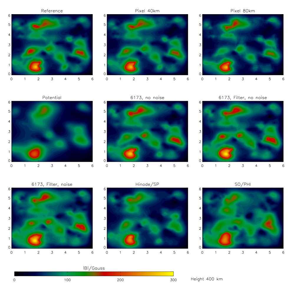
Figure 3: Same as Fig. 2, but $400km$ above the reference height.

2.7 Figures of merit

Schrijver et al. (2006) introduced several figures of merit to compare the results of magnetic field extrapolation codes (a 3D-vector field ${\bf b}$) with a reference solution ${\bf B}$.

• Vector correlation:

  $$C_{\rm vec}=\sum_{i}{\bf B_{i}}\cdot{\bf b_{i}}/\left(\sum_{i}|{\bf B_{i}}|^{2}\sum_{i}|{\bf b_{i}}|^{2}\right)^{1/2},$$ (5)

  where $i$ corresponds to all grid points in the entire 3D computational box.

• Total magnetic energy of the reconstructed field ${\bf b}$ normalized by the energy of the reference field ${\bf B}$:

  $$\epsilon=\frac{\sum_{i}|{\bf b_{i}}|^{2}}{\sum_{i}|{\bf B_{i}}|^{2}}.$$ (6)

• We also compute the linear Pearson correlation $C$ of the total magnetic field strength $|B|$ at the heights 100km, 400km and 800km above the reference height, $Z_{ref}$, respectively.

Two vector fields agree perfectly if $C_{\rm vec}$, $\epsilon$ and the Pearson correlation coefficients are unity.

3 Results

Table 2 contains the different quantitative measures which compare the different reconstructed field from synthetic observations with the reference field (extrapolations from ideal data). Column 2 contains the vector correlation $C_{\rm vec}$, column 3 the normalized magnetic energy $\epsilon$, and columns 4-6 the linear Pearson correlation $C$ of the total magnetic field strength $|B|$ at the heights 100km, 400km and 800km above the reference height, $Z_{ref}$, respectively.

Figs 2 and 3 show contourplots of the magnetic field strength $|{\bf B}|$ at $100$ km and $400$ km above $Z_{ref}$ respectively.

3.1 MHD cases

In the first $4$ images of Figs 2 and 3 we compare the nonlinear force-free 3D magnetic field reconstructed from ideal data (extracted from the MHD simulations at $Z_{ref}$, called Reference in Table 2 and in Figs. 2, 3) with a potential field extrapolation also starting from ideal data (Potential) and nonlinear force-free computations starting from magnetic field maps obtained from the inversion of synthetic Stokes profiles and MHD cases. Potential fields are often calculated in addition to NLFFF, because they contain the minimum energy for given vertical boundary conditions and the free energy of a NLFF-field above that of a potential field has relevance for coronal eruptions.

As seen in Table 2 and in Figs. 2 and 3 the computations with reduced spatial resolution of $40$ km pixels show almost perfect agreement, while $80$ km pixels still provide an excellent correspondence. The correlation with the reference field is better higher in the atmosphere, which is not surprising since small-scale field structures at the lower boundary do not propagate very high and the larger scales are less affected by the binning to larger horizontal pixels. The magnetic energy is underestimated because small scale fields and currents at low heights, which contribute significantly to the total magnetic energy, are not resolved here.

3.2 Dependence on spectral line, noise and spectral sampling

The remaining images in Figs. 2 and 3 and the remaining entries in Table 2 apply to extrapolations starting from magnetic maps obtained from inversions of synthetic spectral lines. The first $3$ of these images (marked 6173 no noise, Filter no noise, Filter noise in Figs. 2 and 3) and the whole middle part of Table 2 are test cases for which we move step-by-step away from ideal conditions (i.e. $\mathbf{B}$ obtained directly from the MHD simulations) towards more realism, i.e. introducing various instrumental effects.

The first such step is to invert the synthetic line profiles directly, without any further manipulation (ideal spectropolarimeter). This step introduces uncertainties due to the inversion process per se (e.g. by the fact that asymmetric Stokes profiles are fit assuming purely symmetric or antisymmetric ones), the fact that the line samples a range of heights, and the dependence of the line formation height on the type of solar feature.

The inversion of Stokes spectra expected from an ideal spectropolarimeter leads to an agreement with the reference within a few percent for the vector correlation and we can estimate the magnetic energy with an accuracy of one percent for the $6173.3$ Å line. The magnetic energy is an important quantity because it tells us how much free energy is maximally available for eruptive phenomena like flares and coronal mass ejections. The high accuracy achieved in this case is particularly encouraging since it shows that applying a simple Milne-Eddington inversion to the often highly asymmetric profiles (sometimes showing multiple lobes in Stokes V) gives sufficiently accurate results and that the fluctuating height at which the magnetic field is obtained does not significantly influence the extrapolations (note that the situation may be different in a sunspot with its rather deep Wilson depression). This result implies that most of the inaccuracies in the extrapolations are due to limitations in the instrumentation and not because it is in principle not possible to extract the information from the observations.

As Table 2 shows there is little to choose between the two $g=2.5$ Zeeman triplets $\lambda 6302.5$ Å line and $\lambda 6173.3$ Å. The field extrapolated from the magnetic field maps derived from either of them correlate very well with the reference field. Using the $\lambda 6173.3$ Å lines leads to a slightly better estimate of the magnetic energy, but all in all the necessity of using the Zeemann effect in a spectral line by itself only leads to errors of a few percent . The addition of noise at a level of $10^{-3}$ of the continuum intensity $I_{c}$, which is typical of modern spectropolarimetric observations, has only a small effect. Note that by adding an equal amount of photon noise to all Stokes parameters we are producing a much lower S/N ratio in the linearly polarized $Q$ and $U$ profiles than in Stokes $V$ due to the smaller signal in the former. The influence of noise of a given amplitude also depends heavily on the magnetic flux in the box for which we extrapolate. With $\langle B\rangle\approx 150$ G the chosen snapshot corresponds to an average plage region. We expect that the same amount of noise will have a considerably stronger effect when applied to the weaker Stokes profiles present in the quiet sun.

It is of particular interest if measurements in limited wavelength bands and at reduced wavelength resolution, typical of filter polarimeters (filter magnetographs), are acceptable for extrapolations. One advantage of such instruments is that they allow time series of a whole region to be recorded at high cadence. Of particular relevance for magnetic extrapolations is the fact that filter polarimeters record the Stokes vector over the full field of view. This overcomes the main shortcoming of spectropolarimeters, namely that they need to scan a region step by step, so that by the time the second footpoint of a loop is scanned the first may have evolved considerably. These advantages of filter instruments come at the price of a reduced spectral resolution and limited spectral sampling. An extensive series of tests by one of us (L. Yelles) using various MHD simulation snapshots has shown that observations at 5 wavelength points in the line plus one at the continuum should be adequate to obtain the magnetic field vector reliably.

The computations carried out here suggest that this is also true for the magnetic field extrapolated from vector magnetograms obtained from filter instruments. According to Table 2 and Figs. 2 and 3 the application of $100$ mÅ broad filters to 5 locations in the Fe I $6173.3$ Å line and additionally to a nearby continuum position gives an extrapolated nonlinear force-free field that differs only slightly from the results obtained with the full line profile. The magnetic energy is overestimated by at most $6\%$ for a filter width $<100$ mÅ and at least 5 sampling points in the line and one in the nearby continuum.

Noise has a somewhat larger effect on filter polarimeter measurements than on spectropolarimetric ones, as can be judged from Table 2. In particular, the magnetic energy is affected, being more than $2\times$ less accurate than for spectropolarimetric measurements. If we take the effect of photometric noise of $10^{-3}I_{c}$ in all Stokes parameters into account we overestimate the magnetic energy by $10\%$. The somewhat higher magnetic energy for these cases is probably a result of stronger currents in the photosphere, which are created by a less accurate computation of the horizontal photospheric field during the inversion. The total vertical magnetic field $\int|B_{z}|\;dxdy$ in the photosphere is underestimated by $7\%$ after inversion of a set of filter images (irrespective of whether noise is applied or not). The total vertical current $\int\left|\frac{\partial B_{y}}{\partial x}-\frac{\partial B_{x}}{\partial y}\right|\;dxdy$ is overestimated by $42\%$ and $262\%$ without and with noise, respectively. Most of these spurious currents produced by spectral line inversions fluctuate on very small scales so that they either are noise, or behave like that. Consequently, they are not transported into the corona. The preprocessing routine takes care of this problem and most of the spurious currents vanish. After preprocessing the total current is overestimated by $2\%$ and $9\%$ for inversions without and with noise, respectively.

3.3 Hinode-like cases

Finally, as discussed in this and the following subsection, we add more realism into the synthetic observations by employing parameters that are appropriate to high resolution instruments. In this section we consider the important case of the spectropolarimeter on Hinode (see also Section 2.3).

Taking a finite spatial resolution (pixel size 110 km) and spectral smearing into account naturally leads to less accurate results (rows marked Hinode/SP in Table 2). We find that we cannot reconstruct the magnetic energy accurately for these cases, because small scale magnetic fields are not adequately resolved. We get, however, a reasonable estimate of the correct magnetic field in higher layers of the atmosphere. For the most involved case (Hinode-like spectropolarimeter with a noise of $10^{-3}I_{c}$ and a pixel size of 110 km) we find an error of $16\%,\,5\%$ and $1\%$ at the heights 100, 400 and 800 km above $Z_{\rm ref}$, respectively. The limited resolution avoids accurate reconstructions of low-lying small scale features, but gets the higher lying field approximately correctly. At heights above 400 km even the most involved and noisy nonlinear force-free reconstruction considered here has an accuracy, which is three times better than with a potential field reconstruction starting from a perfectly known lower boundary.

3.4 SO/PHI-like cases

We consider instrumental effects appropriate to the PHI instrument on Solar Orbiter such as the finite spectral resolution and sampling by a Fabry-Perot interferometer, finite spatial resolution of approximately 160 km (pixel size 80 km) on the Sun and photon noise at a level of $10^{-3}\times\frac{1}{\sqrt{I_{c}}}$. Details are given in Sect. 2.4. The extrapolated magnetic field displays a very similar spatial distribution as that based on the inversion of ideal line profiles. On the whole, the influence of degrading the spatial resolution to a pixel size of $80$ km (denoted as Filter+Noise in Figs. 2, 3) introduces a similar level of inaccuracy in the extrapolated field as the uncertainties in $B_{x},B_{y},B_{z}$ at the lower boundary introduced by instrumental effects and the inversion of the line profiles. But even for this most involved cases, with comparatively low resolution, instrument effects and noise, the agreement with the reference is better than a potential field computed from ideal data at the lower boundary. The better correspondence of $\epsilon$ with the reference value than for Hinode is likely due to the somewhat higher spatial resolution expected for PHI. This suggests that for accurate estimates of the magnetic energy it is more important to achieve high spatial resolution than completely accurate line profiles. The field at 100 km above $Z_{\rm ref}$ and partly at 400 km is better reproduced for Hinode/SP-like parameters than for the SO/PHI case. Obviously, for this it is better to have the full line profile (in particular when noise is included).

4 Conclusions

We have investigated how strongly inaccuracies in the lower magnetic boundary, introduced by measurement and analysis errors of the Stokes profiles influence the computation of nonlinear force-free coronal magnetic fields.

We find that instrument effects and noise influence the horizontal component of the photospheric magnetic field vector stronger than the vertical field. We find that non-linear force-free fields extrapolated from ideal data and from the inversion of Stokes profiles deviate more strong at low heights. In particular, a limited spatial resolution influences the lowest layers the strongest. Higher in the atmosphere we found a very good agreement (correlation better than $0.98$) with extrapolations from ideal data. We find that for an accurate estimation of the magnetic energy a high spatial resolution is more important than a high spectral resolution.

These basic findings apply to magnetic vector maps obtained from both, spectropolarimetric data, such as provided by Hinode/SP, and filter magnetographs, such as to be provided by SO/PHI or SDO/HMI.

Figure 4: Scatter plot displaying how errors in the photosphere affect the accuracy of the 3D magnetic field reconstruction. Shown is the 3D vector correlation against the 2D vector correlation in the photosphere. The solid line corresponds to a linear fit and the dotted line corresponds to identical 2D and 3D correlations.

Finally, we would like to determine how errors in the photosphere influence the quality of the 3D reconstruction. For this aim we show a scatter plot in Fig. 4 to compare the 2D-vector correlation in the photosphere (Table 1) with the 3D vector correlation of the reconstructed coronal magnetic field (Table 2). The solid line in Fig. 4 shows a linear fit to the data points and the dotted line corresponds to equal 2D and 3D correlations. As one can see from this figure the relation between the accuracy of the photospheric and coronal field is linear, but not identical. In particular, the correlation of the full 3D field drops off more slowly than the photospheric correlation, so that extrapolations based on a filter instrument with noise (which gives the least accurate photospheric field) are more accurate than the vector magnetograms they are based on.

It would be interesting to repeat this study on larger spatial scales, reaching sizes typical of observed vector magnetograms, as soon as the corresponding radiative MHD-simulations become available (with a similar grid size as the simulations employed here). There is also a need to investigate quiet Sun regions, coronal holes and active regions separately. In particular, our results may not apply when considering extrapolations starting from regions containing sunspots due to their much larger Wilson depression and rather different temperature structure, which influence the line formation height and the line formation in general. We have also not considered subtle, but possibly important effects such as the evolution of the field during the scan of an active region by the slit of a spectropolarimeter, or the evolution of a line profile during the spectral scan of a filter instrument.

One might also consider investigating the lower layers of the solar atmosphere, where the plasma is not force-free, in more detail and taking non-magnetic forces into consideration for the magnetic field extrapolation. A first step in this direction has recently been taken by Wiegelmann & Neukirch (2006), who developed a magnetohydrostatic extrapolation code. For an application to data we require, however, more information regarding the nature of the non-magnetic forces (e.g., pressure gradients and gravity).