Weakly chiral networks and 2D delocalized states in a weak magnetic field

Abstract

We study numerically the localization properties of two-dimensional electrons in a weak perpendicular magnetic field. For this purpose we construct weakly chiral network models on the square and triangular lattices. The prime idea is to separate in space the regions with phase action of magnetic field, where it affects interference in course of multiple disorder scattering, and the regions with orbital action of magnetic field, where it bends electron trajectories. In our models, the disorder mixes counter-propagating channels on the links, while scattering matrices at the nodes describe exclusively the bending of electron trajectories. By artificially introducing a strong spread in the scattering strengths on the links (but keeping the average strength constant), we eliminate the interference and reduce the electron propagation over a network to a classical percolation problem. In this limit we establish the form of the    disorder – magnetic field    phase diagram. This diagram contains the regions with and without edge states, i.e. the regions with zero and quantized Hall conductivities. Taking into account that, for a given disorder, the scattering strength scales as inverse electron energy, we find agreement of our phase diagram with levitation scenario: energy separating the Anderson and quantum Hall insulating phases floats up to infinity upon decreasing magnetic field. From numerical study, based on the analysis of quantum transmission of the network with random phases on the links, we conclude that the positions of the weak-field quantum Hall transitions on the phase diagram are very close to our classical-percolation results. We checked that, in accord with the Pruisken theory, presence or absence of time reversal symmetry on the links has no effect on the line of delocalization transitions. We also find that floating up of delocalized states in energy is accompanied by doubling of the critical exponent of the localization radius. We establish the origin of this doubling within classical-percolation analysis.

I Introduction

I.1 Levitation scenario

Scaling theory of localization AALR predicts that evolution with size, $L$, of the conductivity, $\sigma$, (in the units of $e^{2}/2\pi\hbar$) of a 2D sample is governed only by the value of $\sigma$, regardless of the type of disorder in the sample, i.e.,

$$\frac{\partial\sigma}{\partial\ln L}=\sigma\cdot\beta(\sigma).$$ (1)

Together with initial condition, $\sigma{\big{|}}_{L\sim l}=\sigma_{0}=k_{\scriptscriptstyle F}l$, where $k_{\scriptscriptstyle F}$ is the Fermi momentum, and $l$ is the transport mean free path, Eq. (1) suggests that, in zero magnetic field, where $\beta(\sigma)=-2/(\pi\sigma)$, localization radius of electron states is given by

$$\ln\Bigl{(}\frac{\xi_{o}}{l}\Bigr{)}=\frac{\pi\sigma_{0}}{2}=\frac{\pi}{2}k_{\scriptscriptstyle F}l.$$ (2)

With increasing magnetic field, when $\beta(\sigma)$ crosses from the orthogonal to the unitary form, $\beta_{u}(\sigma)=-1/(\pi\sigma)^{2}$, the localization radius crosses over from $\xi_{o}$ to $\xi_{u}$, given by

$$\ln\Bigl{(}\frac{\xi_{u}}{l}\Bigr{)}=\pi^{2}\sigma_{0}^{2}=\pi^{2}(k_{\scriptscriptstyle F}l)^{2}.$$ (3)

Crossover takes place when weak localization is suppressed, i.e., when the magnetic flux through the vector area spanned by the electron travelling diffusively over the area $\sim\xi_{o}^{2}$, is of the order of the flux quantum. With vector area being $\sim\xi_{o}l$, we get the following estimate for crossover magnetic field

$$\omega_{c}\tau=\frac{l}{\xi_{o}}\sim\exp\left(-\frac{\pi}{2}k_{\scriptscriptstyle F}l\right),$$ (4)

where $\omega_{c}$ is the cyclotron frequency, and $\tau$ is the scattering time.

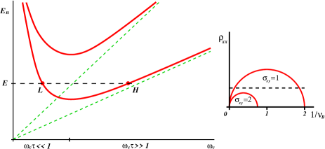
Figure 1: (Color online) Left: Energy position of two lowest delocalized states, $E_{0}$ and $E_{1}$, as a function of magnetic field, $\omega_{c}$, as predicted in Ref. Khmelnitskii, . At a given $E$, delocalization transition occurs at low field (point $L$) and at high field (point $H$). Right: Same dependencies, replotted in the axis inverse filling factor vs. zero-field resistivity, constitute a part of the global phase diagram Ref. Kivelson, . Depending on $\rho_{xx}^{0}$, the system undergoes a sequence of transitions, $0\rightarrow 1\rightarrow 0$ or $0\rightarrow 1\rightarrow 2\rightarrow 1\rightarrow 0$.

The origin of the crossover Eq. (4) is that the paths, which interfere in a zero field, acquire field-induced random Aharonov-Bohm phases. Justification for considering exclusively the phase action of magnetic field is that in high-mobility samples with $k_{\scriptscriptstyle F}l\gg 1$ the crossover field is so weak that its orbital action can be neglected. It is a very delicate fact that, after the crossover, this orbital action causes a drastic change of the eigenstates even for classically weak magnetic fields, $\omega_{c}\tau\ll 1$. This conclusion was drawn by Khmelinitskii Khmelnitskii from the analysis of the renormalization group flows Khmelnitskii ; pru83 . Originally, these equations were derived to describe quantization of the Hall conductivity in a strong-field limit, $\omega_{c}\tau\gg 1$,

$$\frac{\partial\sigma_{xx}}{\partial\ln L}=-\frac{1}{2\pi^{2}\sigma_{xx}}-\sigma_{xx}^{2}{\cal D}e^{-2\pi\sigma_{xx}}\cos(2\pi\sigma_{xy}),$$ (5)

$$\frac{\partial\sigma_{xy}}{\partial\ln L}=-\sigma_{xx}^{2}{\cal D}e^{-2\pi\sigma_{xx}}\sin(2\pi\sigma_{xy}),$$ (6)

where $\sigma_{xx}$ and $\sigma_{xy}$ are, respectively, the diagonal and non-diagonal components of the conductivity tensor, and ${\cal D}$ is a dimensionless constant. First term of Eq. (5) is the same as in Eq. (1) with unitary $\beta(\sigma)$. It originates from interference: two paths corresponding to the same scatterers but different sequences of scattering events interfere even in the presence of Aharonov-Bohm phases. Second term reflects the orbital action of magnetic field (Lorentz force); by curving electron trajectories it tends to destroy the interference. Quantum Hall transition between $\sigma_{xy}{\big{|}}_{L\rightarrow\infty}=n$ and $\sigma_{xy}{\big{|}}_{L\rightarrow\infty}=n+1$ takes place when the “phase” and “orbital” terms compensate each other. Khmelnitskii’s treatment Khmelnitskii is equivalent to solving Eqs. (5), (6) together with classical Drude initial condition,

$$\sigma_{xx}{\big{|}}_{L\sim l}=\frac{\sigma_{0}}{1+(\omega_{c}\tau)^{2}},\qquad\sigma_{xy}{\big{|}}_{L\sim l}=\frac{\sigma_{0}\,(\omega_{c}\tau)}{1+(\omega_{c}\tau)^{2}},$$ (7)

which yields the positions of delocalized states

$$E_{n}=\hbar\omega_{c}\left(n+\frac{1}{2}\right)\left[1+\frac{1}{(\omega_{c}\tau)^{2}}\right].$$ (8)

As shown in Fig. 1 for $n=0,\,1$, the high-field part, $\omega_{c}\tau\gg 1$, of $E_{n}$ follows the centers of Landau levels, while the low-field part, $E_{n}\tau\approx(n+1/2)(\omega_{c}\tau)^{-1}$, “floats up” as $\omega_{c}\tau\rightarrow 0$. Such a behavior of critical values of $k_{\scriptscriptstyle F}l=E_{\scriptscriptstyle F}\tau$ in vanishing field is usually called levitation of delocalized states Lev_1 . More specifically, it is expected that, upon increasing magnetic field above the crossover Eq. (4), localization radius, $\xi(\omega_{c})$, diverges in the vicinity of discrete values $\omega_{c}\tau=(n+1/2)(k_{\scriptscriptstyle F}l)^{-1}$, changing from unitary $\xi_{u}$ to infinity and returning back to $\xi_{u}$. Recasting Eq. (8) into the dependence, $\rho^{0}_{xx}=\sigma_{0}^{-1}$, versus the inverse filling factor, $\nu^{-1}_{\scriptscriptstyle B}=\omega_{c}/(2E_{\scriptscriptstyle F})$, yields a system of semicircles

$$\rho_{xx}^{2}+\left(\frac{1}{\nu_{\scriptscriptstyle B}}-\frac{1}{n+1/2}\right)^{2}=\frac{1}{(n+1/2)^{2}},$$ (9)

shown in Fig. 1 inset, which is a part of the global phase diagram Kivelson . This diagram suggests that for high enough $\rho^{0}_{xx}$, i.e., for strong disorder, the resistance $\rho_{xx}(\omega_{c})$ grows monotonically. Upon decreasing $\rho^{0}_{xx}$, below a certain threshold value, Fig. 1 (e.g., by applying the gate voltage) $\rho_{xx}(\omega_{c})$ exhibits two quantum Hall peaks. For $\rho^{0}_{xx}$ smaller than the second threshold, Fig. 1, $\rho_{xx}(\omega_{c})$ exhibits four peaks, and so on. By now, such a behavior (two peaks in $\rho_{xx}(\omega_{c})$ dependence for small enough $\rho^{0}_{xx}$) was reported in a number of experimental papers Refs. Jiang92, ; Jiang93, ; Jiang93PRL, ; Jiang95PRL, ; Jiang95, ; Jiang98, ; Kravchenko95, ; Wang94, ; Hughes94, ; ShaharLev, . On the other hand, theoretical numerical studies xiong01 ; liu96 ; yang96 ; sheng97 ; sheng98 ; sheng00 ; koschny01 ; Wen ; wan01 ; Sch aimed at revealing levitation on a microscopic level, are less conclusive Huckestein00 . The only established fact is the tendency Shahbaz95 ; Kagalovsky95 ; kagalovsky97 ; Gramada96 ; Haldane97 ; Fogler98 ; Schulz for floating up of delocalized states upon decreasing $\omega_{c}$ in the strong-field domain, where Landau levels are still well-defined. This tendency is due to disorder-induced mixing of the neighboring well-resolved Landau levels.

I.2 Network models

First numerical verification KramMac of one-parameter scaling Eq. (1) was performed within the Anderson model Anderson58 . Physically, this model corresponds to realizations of disorder in which scatterers have random strength, while positional disorder is eliminated by placing scatterers on the lattice. In other words, the phase acquired by electron between two subsequent scattering acts is assumed to be the same. Important is that the minimal model Anderson58 , in which disorder is characterized by a single dimensionless parameter, spread of the site energies in the units of bandwidth, captures all features of a generic random potential.

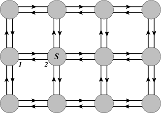
Figure 2: In non-chiral network model, confining potential restricts electron motion to the links. All the scattering matrices $S$ at the nodes are the same. Positional disorder is emulated by randomness of phases acquired on the links. Depending on symmetry class, the phases between the points 1 and 2 are either the same or different.

Another minimal description of disorder is at the core of scattering approach to localization introduced by B. Shapiro Shapiro . Microscopic realization of the network Ref. Shapiro, requires restricting the electron motion by a confining potential, as illustrated in Fig. 2. This confining potential ensures that there are only four possible outcomes of scattering, which takes place at the nodes. In contrast to Anderson model, all scatterers at the nodes of network are assumed identical, while positional disorder is maximally strong. This is achieved by assuming that phases, accumulated between the neighboring nodes, are completely random. Within the network model description, a physical parameter, $(k_{F}l)^{-1}$, is emulated by $1-T$, where $T$ is the transmission of the node. One of the apparent successes of the network model description of disordered systems was the demonstration SO of the zero-field localization-delocalization transition in 2D system with spin-orbit scattering. Formal origin of this transition is the change of sign of $\beta(g)$ in Eq. (1) in the presence of spin-orbit scattering HikLar

Network-model approach is especially well suited for the description of the quantum Hall transition in a strong magnetic field. As was pointed out by Chalker and Coddington CC (CC), in this case, unlike zero magnetic field, the links of the network acquire a natural physical meaning, namely, they coincide with equipotential lines Kazarinov ; Iordansky ; Trugman of the bare smooth (on the scale of magnetic length) random potential. This is due to the field-induced quenching of kinetic energy of electron, rather than due to artificially imposed confining potential. In addition, in strong magnetic field, the motion along each link, representing the drift of the Larmour circle, is unidirectional. Nodes in the of the CC network also have a transparent meaning: they represent saddle points of the random potential, where equipotentials come as close as magnetic length. Various aspects of the Quantum Hall transition, relevant to experiment wei90 ; pan97 ; schaijk00 ; koch91 ; Tsui05 ; Tsui09 ; Cobden96 ; hohls02 ; peled02 , e.g., divergence of the localization radius (scaling CC ; Kivelson93 ; Ohtsuki09 ), critical statistics of energy levels klesse , mesoscopic conductance fluctuations Jovanovic96 ; Fisher97 , point-contact conductance zirnbauer99 , were studied theoretically using the CC model KramOhtsKet .

Testing the levitation scenario microscopically requires to construct a minimal weakly chiral network model, which captures the physics encoded in the system Eq. (5), namely competition between interference-induced localization and orbital-induced curving asymmetry in the scattering to the “left” and to the “right”. Construction of such a network and study of its localization properties is the objective of the present paper. On the physical grounds, the desired description should contain only two parameters, $k_{\scriptscriptstyle F}l$ and $\omega_{c}\tau$. Short communication on the results reported below can be found in Ref. We, .

II Reformulation of non-chiral network model

We achieve the goal of constructing a minimal weakly-chiral network model in two steps. First we reformulate the standard non-chiral network model Fig. 2 by separating each node into the regions with backscattering and left-right scattering. As a second step we incorporate weak chirality in the form of imbalance between scattering to the left and scattering to the right.

In a standard non-chiral network model Fig. 2 the scattering at the node is described by $4\times 4$ unitary scattering matrix. This matrix can be parameterized by three independent numbers, e.g., as follows:

$$S=\left(\begin{array}[]{cccc}r&-d_{1}&-t&-d_{2}\\ d_{1}&r&d_{2}&-t\\ t&-d_{2}&r&d_{1}\\ d_{2}&t&-d_{1}&r\end{array}\right),$$ (14)

where reflection, $r$, transmission, $t$, and deflection coefficients, $d_{1}$, $d_{2}$, are all real and satisfy the flux conservation condition

$$r^{2}+t^{2}+d_{1}^{2}+d_{2}^{2}=1.$$ (15)

Isotropy requires that $d=d_{1}=d_{2}$, so that the scatterer is characterized by only two independent parameters, say $t$ and $d$. The model belongs to the orthogonal symmetry class if the phase, $\varphi_{12}$, accumulated upon propagation $1\rightarrow 2$ between the scatterers $1$ and $2$, Fig. 2, is equal to the phase, $\varphi_{21}$, accumulated upon propagation $2\rightarrow 1$. Otherwise, it belongs to the unitary class.

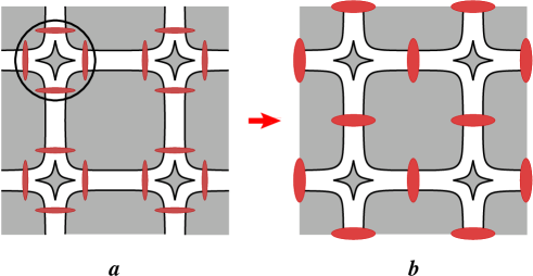
Figure 3: (Color online) Construction of weakly chiral network model. a: Node scattering matrix is decomposed into four ”reflectors” and a ”junction”. b: Final network model upon combining two reflectors on a given link into one reflector.

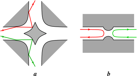
Figure 4: (Color online) a: Microscopic realization of the junction matrix Eq. (18). The junction is defined by the confinement potential (shaded area); rhomboidal scatterer at the center ensures that each incident wave is deflected only to the left or to the right. b: Scattering on a link, described by matrix Eq. (32), can be modelled with a point contact.

Full localization of the eigenstates in 2D, predicted by the scaling theory AALR , manifests itself in vanishing transmission of the network for all sets of $t$ and $d$. The degree of localization is governed by the conductance SO

$$k_{\scriptscriptstyle F}l=\frac{1}{2}\,\frac{t^{2}+d^{2}}{1-t^{2}-d^{2}}.$$ (16)

If $d$ and $t$ are small, localization is strong (within one plaquette). Conversely, for $t$ close to $1$, electron changes the direction of propagation after $\sim(1-t^{2})^{-1}\gg 1$ scattering acts, which corresponds to high conductance, $k_{\scriptscriptstyle F}l\gg 1$, and exponentially large localization radius. It is important to mention one particular case, namely, $t\ll 1$ and $d\approx 1/\sqrt{2}$. According to Eq. (16), this case of almost complete deflection, with weak reflection and transmission, should correspond to strong localization. This is, however, not the case. In fact, the states become progressively delocalized as $d$ approaches the value $1/\sqrt{2}$. This conclusion can be drawn from Ref. Bocquet, , where the corresponding limit of the network model has been studied. Since the case $d\approx 1/\sqrt{2}$ will play an important role in our construction later on, we discuss a seeming contradiction to the scaling in this case in Appendix.

Note in passing, that the parametrization Eq. (14) reflects the Born scattering (for $d_{1}=d_{2}$), where the probabilities of deflection, forward, and backward scattering are independent of the direction of incidence. This is certainly not the general case of potential scattering. In fact, one can relax the condition $d_{1}=d_{2}$ for a given node and ensure global isotropy by requiring that the scattering to the left and to the right are equally probable on average (over the nodes).

Our reformulation of the network model is illustrated in Fig. 3. We start with specifying scattering matrices at the nodes of Fig. 2 as systems of four ”reflectors” and one junction, Fig. 3. Each reflector mixes only two channels on the corresponding link, so that its scattering matrix

$${\cal P}_{0}=\left(\begin{array}[]{cc}\sqrt{1-p_{0}}&\sqrt{p_{0}}\\ \\ -\sqrt{p_{0}}&\sqrt{1-p_{0}}\end{array}\right)$$ (17)

is $2\times 2$, where $p_{0}$ is the power reflection coefficient. The junction, Fig. 4, does not transmit or reflect incoming waves, but rather scatters them either to the left or to the right with equal probability, $1/2$. The corresponding $4\times 4$ scattering matrix has the form

$${\cal S}_{0}=\left(\begin{array}[]{cccc}0&-\frac{1}{\sqrt{2}}&0&-\frac{1}{\sqrt{2}}\\ \frac{1}{\sqrt{2}}&0&\frac{1}{\sqrt{2}}&0\\ 0&-\frac{1}{\sqrt{2}}&0&\frac{1}{\sqrt{2}}\\ \frac{1}{\sqrt{2}}&0&-\frac{1}{\sqrt{2}}&0\\ \end{array}\right).$$ (18)

It is important to demonstrate that the combination of a junction and four reflectors which is characterized by a single parameter, $p_{0}$, corresponds to the effective node of the scattering matrix with appropriate symmetry. Let us denote with $\phi_{i}$ the phase accumulated between the junction and reflector on the link $i$, $i=1,..,4$, Fig. 3a. For potential scattering with time-reversal symmetry preserved, the phase accumulated between the reflector and the junction is the same $\phi_{i}$, as for propagation between the junction and reflector. Then the effective node scattering matrix assumes the form

$${\cal S}=\left(\begin{array}[]{cccc}R^{1}_{2,4}&-D_{1,2}&T_{4,2}&D_{1,4}\\ \\ D_{2,1}&R^{2}_{3,1}&D_{2,3}&T_{3,1}\\ \\ T_{2,4}&-D_{3,2}&R^{3}_{4,2}&D_{3,4}\\ \\ D_{4,1}&T_{1,3}&-D_{4,3}&R^{4}_{1,3}\end{array}\right),$$ (26)

where the deflection, transmission, and reflection coefficients are defined as

$$D_{i,j}=\frac{\sqrt{2}(1-p_{0})}{\cal N}\bigl{(}e^{i(\phi_{i}+\phi_{j})}+p_{0}e^{i(2\psi-\phi_{i}-\phi_{j})}\bigr{)},$$ (27)

$$T_{i,j}=2i\frac{\sqrt{p_{0}}(1-p_{0})}{\cal N}\sin(\phi_{i}-\phi_{j})e^{2i\psi},$$ (28)

$$R^{i}_{j,k}=\frac{\sqrt{p_{0}}}{\cal N}\Bigl{[}\bigl{(}e^{2i\phi_{i}}+p_{0}e^{2i(\psi-\phi_{i}-\phi_{j}-\phi_{k})}\bigr{)}\bigl{(}e^{2i\phi_{j}}+e^{2i\phi_{k}}\bigr{)}$$

$$\hskip 56.9055pt+2+2p_{0}e^{2i\psi}\Bigr{]}.$$ (29)

In Eqs. (27)-(29), $\psi=\sum\phi_{i}$ is the net phase; normalization factor is defined as

$${\cal N}=2+2p^{2}_{0}e^{2i\psi}+p_{0}(e^{2i\phi_{1}}+e^{2i\phi_{3}})(e^{2i\phi_{2}}+e^{2i\phi_{4}}).$$ (30)

One can check that the matrix Eq. (26) is unitary. For arbitrary phases, $\phi_{i}$, it does not reduce to the form Eq. (14) with equal reflection, transmission, and deflection probabilities for all directions of incident channels. Global isotropy is restored upon averaging over $\phi_{i}$. For example, if we choose a particular set, $\phi_{1}=\phi_{2}=\pi/4$, $\phi_{3}=\phi_{4}=-\pi/4$, the matrix Eq. (26) assumes the form

$$\hat{{\cal S}}_{0}=\frac{1}{1+p^{2}_{0}}\left(\begin{array}[]{cccc}-\sqrt{p_{0}}(1+p_{0})&-\frac{i}{\sqrt{2}}(1-p_{0})^{2}&-i\sqrt{p_{0}}(1-p_{0})&-\frac{1}{\sqrt{2}}(1-p^{2}_{0})\\ \\ \frac{i}{\sqrt{2}}(1-p_{0})^{2}&-\sqrt{p_{0}}(1+p_{0})&\frac{1}{\sqrt{2}}(1-p^{2}_{0})&-i\sqrt{p_{0}}(1-p_{0})\\ \\ -i\sqrt{p_{0}}(1-p_{0})&-\frac{1}{\sqrt{2}}(1-p^{2}_{0})&-\sqrt{p_{0}}(1+p_{0})&-\frac{i}{\sqrt{2}}(1-p_{0})^{2}\\ \\ \frac{1}{\sqrt{2}}(1-p^{2}_{0})&-i\sqrt{p_{0}}(1-p_{0})&\frac{i}{\sqrt{2}}(1-p_{0})^{2}&-\sqrt{p_{0}}(1+p_{0})\\ \end{array}\right).$$ (31)

This choice favors deflection $|d_{2}|$ over deflection $|d_{1}|$. The asymmetry between $|d_{2}|$ and $|d_{1}|$ is compensated by realization in which $\phi_{1}=\phi_{2}=-\pi/4$, $\phi_{3}=\phi_{4}=\pi/4$; for this realization, $|d_{1}|$ and $|d_{2}|$ switch places. It is seen from Eq. (26) that presence of reflectors eliminates the singular character of junction matrix ${\cal S}_{0}$ by restoring finite forward and backward scattering probabilities. In other words, the use of the matrix Eq. (26) instead of node matrix Eq. (14) would reveal full localization of electron states at any $p_{0}$. However, for small $p_{0}$, the parametric space of matrices Eq. (26) is restricted to small transmission and reflection, $|t|^{2}\sim|r|^{2}\sim p_{0}$, the domain where the mean free path Eq. (16) is $\sim 1$. Despite what Eq. (16) predicts, we will get large values of localization length, $\xi(p_{0})$, in the domain $p_{0}\ll 1$.

We complete our reformulation of the non-chiral network model by observing that the random phases on the links between two neighboring reflectors can be incorporated into $\phi_{i}$. This allows one to combine the two reflectors on the same link into a single effective $2\times 2$ scatterer on this link, as it is shown in Fig. 3b. The corresponding effective scattering matrix,

$${\cal P}=\left(\begin{array}[]{cc}\sqrt{1-p}&\sqrt{p}\\ \\ -\sqrt{p}&\sqrt{1-p}\end{array}\right),$$ (32)

has the same form as Eq. (17) with

$$p=\frac{4p_{0}}{(1+p_{0})^{2}}.$$ (33)

The resulting network consisting of junctions at nodes and effective scatterers on the links is shown in Fig. 3b. On the microscopic level, the node ${\cal S}_{0}$ corresponds to the junction with confinement shown in Fig. 4a, while the link matrix ${\cal P}$ corresponds to point-contact confinement, Fig. 4b.

III Orbital action of a weak magnetic field

As was discussed in the Introduction, weak magnetic field in which delocalization transition takes place, is already strong enough to drive random phases on the links of the network Fig. 3b into the unitary class. We also need to incorporate the Lorentz-force effect of magnetic field. For free electrons, the Lorentz force curves their trajectories. In the network Fig. 3b it affects the properties of junctions only, leading to imbalance between deflection to the left and deflection to the right. Note, that general properties of a four-terminal junction in magnetic field were previously studied in Refs. Ravenhall, ; Baranger, ; Beenakker, for various forms of confinement potential in relation to experiments Timp87 ; Roukes87 ; Chang88 ; Ford88 ; Simmons88 on the Hall quantization in narrow channels.

In order to incorporate orbital action of magnetic field into the general network Fig. 2, one has to place a weakly chiral $S$-matrix into each node. A possible form of such $S$-matrix is

$$S_{ch}=\left(\begin{array}[]{cccc}r_{1}&d_{2}&t_{3}&D_{4}\\ D_{1}&r_{2}&d_{3}&t_{4}\\ t_{1}&D_{2}&r_{3}&d_{4}\\ d_{1}&t_{2}&D_{3}&r_{4}\end{array}\right),$$ (38)

where the complex coefficients have absolute values

$$|r_{i}|=r,\quad|D_{i}|=D,\quad|d_{i}|=d,\quad|t_{i}|=t;$$

$$r^{2}+D^{2}+d^{2}+t^{2}=1.$$ (39)

If magnetic field whirls electrons, say, to the right, one has $D>d$. For example, one can choose the following realizations of the above chiral matrix

$$S_{ch}=\!\left(\begin{array}[]{cccc}r&-d-ib_{-}&t&d+ib_{+}\\ d+ib_{+}&r&-d+ib_{-}&t\\ t&-d+ib_{+}&-r&-d+ib_{-}\\ d+ib_{-}&t&d-ib_{+}&-r\end{array}\right)\!,$$ (44)

provided that $r$, $d$, $t$, and $b_{\pm}$ are positive real numbers ($t>r$) with

$$\frac{b_{-}}{b_{+}}=\frac{t-r}{t+r},\quad r^{2}+t^{2}+2d^{2}+b^{2}_{+}+b^{2}_{-}=1.$$ (46)

We see that the difference between the scattering probabilities to the right and to the left is $|b_{+}|^{2}-|b_{-}|^{2}$. This difference is non-zero, as follows from first identity in Eq. (46). Note that for the particular choice Eq. (38), the ratio, $r/t$, ”controls” the magnetic field strength. Indeed, for $r=0$ we have $b_{+}=b_{-}$.

In general, dimensionless Hall resistance of a junction is expressed via field-dependent elements of the matrix Eq. (14) as follows Ravenhall ; Baranger ; Beenakker

$$R_{H}=\frac{2(d_{1}^{2}-d_{2}^{2})}{(2t^{2}+d_{1}^{2}+d_{2}^{2})^{2}+(d_{1}^{2}-d_{2}^{2})^{2}}.$$ (47)

Note that for the weakly chiral matrix Eq. (44) $R_{H}$ is the same for all directions of incidence. Naturally, the degree of bending action of magnetic field is represented by the difference, $(|d_{1}|^{2}-|d_{2}|^{2})$. The advantage of our reformulation of the network model, described in Sec. II, is that controlled chirality can be incorporated into the network in a natural way upon replacement of the non-chiral matrix ${\cal S}_{0}$, Eq. (18), by

$${\cal S}=\left(\begin{array}[]{cccc}0&-{\scriptstyle\sqrt{1-q}}&0&{\scriptstyle-\sqrt{q}}\\ {\scriptstyle\sqrt{q}}&0&{\scriptstyle\sqrt{1-q}}&0\\ 0&{\scriptstyle-\sqrt{q}}&0&{\scriptstyle\sqrt{1-q}}\\ {\scriptstyle\sqrt{1-q}}&0&{\scriptstyle-\sqrt{q}}&0\end{array}\right).$$ (48)

The matrix ${\cal S}$ is parameterized by a single number, $q=d_{1}^{2}$, which varies between $q=0$ and $q=1$. The Hall resistance is expressed via $q$ as follows:

$$R_{H}=\frac{2q-1}{q^{2}+(1-q)^{2}}.$$ (49)

It is an odd function of

$$\left(\frac{1}{2}-q\right)\propto\omega_{c},$$ (50)

i.e., the difference $(1/2-q)$ can be viewed as a quantitative measure of the magnetic field strength. Concluding this section, the link matrix ${\cal P}$, Eq. (32), parameterized by single parameter, $p$, and the node matrices ${\cal S}$, Eq. (48), parameterized by single parameter, $q$, fully define a minimal network model, Fig. 3b. The advantage of this network is that the disorder and the magnetic field can be ”tuned” independently by changing $p$ and $q$, respectively. We will call this model a p-q model. Localization properties of this model are studied below.

IV p-q model: limit of strong disorder

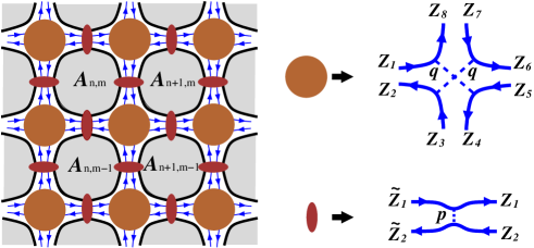
Figure 5: (Color online) Left: In two-channel p-q model, electron motion is restricted to the spaces between forbidden regions $A_{n,m}$. The centers of forbidden regions form a square lattice. Point contacts on the links describe the backscattering by disorder; bend-junctions at the nodes describe the orbital action of magnetic field. Right: Scattering matrices of the junction and of the point contact.

In order to get a qualitative insight into the phase diagram of the quantum p-q model, we start with artificial limit of strong disorder. To define the strong disorder, note that in the original p-q model the values of $p$ and $q$ are the same for all junctions and point contacts. In other words, distribution functions of the parameters $p$ and $q$ are

$$f(p_{i})=\delta(p_{i}-p),\quad f(q_{j})=\delta(q_{j}-q).$$ (51)

By a strong disorder we mean the following distribution of $p$ and $q$,

$$f(p_{i})=p\,\delta(1-p_{i})+(1-p)\delta(p_{i}),$$ (52)

$$f(q_{j})=q\,\delta(1-q_{j})+(1-q)\delta(q_{j}),$$

so that scattering by the point contact and deflection at the junction are still $p$ and $q$ on average. However, unlike Eq. (51), the point contact reflects fully in $p$ percent of cases, and transmits fully in the rest $(1-p)$ percent of cases. Similarly, according to Eq. (52), the junction deflects only to the right in $q^{2}$ percent of cases, deflects only to the left in $(1-q)^{2}$ percent of cases; in the remaining $2q(1-q)$ percent of cases the deflection takes place both to the left and to the right depending on incoming channel.

In considering a strong disorder, our motivation stems from the original CC model, in which the nodes of the network are chiral saddle points. If we introduce disorder in the transmission of saddle points similar to Eq. (52), then, at critical energy, $50\%$ of saddle points will fully transmit, and $50\%$ will fully reflect. For such a disorder, quantum-mechanical interference becomes irrelevant. However, the state will remain critical Kivelson93 , separating the phases with $\sigma_{xy}$ differing by $1$. In this limit of strong disorder, quantum delocalization is replaced by classical percolation transition occurring at the same energy. Our expectation, which will be later supported by numerical simulations, is that similar to CC model, considering the limit of strong disorder of the p-q model will yield the positions of classical delocalization transitions, which coincide with the positions of quantum delocalized states in the original p-q model.

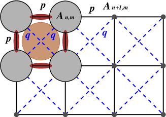
Figure 6: (Color online) Limit of strong disorder. The centers of forbidden regions, $A_{n,m}$ and $A_{n,m-1}$, are connected by the p- bond, while the centers of forbidden regions, $A_{n-1,m-1}$ and $A_{n,m}$, are connected by a q- bond. Electron delocalization reduces to the percolation on the lattice consisting of p- and q- bonds.

The realization with $p_{i}=1$ corresponds to a ”closed” point contact, which reflects incoming waves from both directions. Classically, presence of such a reflecting barrier can be interpreted as a bond installed between the neighboring forbidden regions, $A_{n,m}$ and $A_{n+1,m}$, of confining potential, Fig. 5. Below we will refer to this bond as a p- bond. Similarly, we introduce q- bonds, installed between the forbidden regions, $A_{n,m}$ and $A_{n\pm 1,m\pm 1}$ in Fig. 5. Then, deflection only to the right corresponds to two crossed q- bonds, deflection only to the left corresponds to the situation when all four forbidden regions $A_{n,m}$, defining the junction, are disconnected. One right-diagonal q- bond describes the situation when the junction deflects the fluxes incident from the left and from the right channels to the left, and fluxes incident from the up and down to the right. Similarly, one left-diagonal q- bond signifies reflection from the left and right channels to the right, while the up and down channels are deflected by the junction to the left. Thus we arrive at the percolation problem of connectivity of the forbidden regions $A_{n,m}$ via p- and q- bonds, see Fig. 6. Some limits of this problem are transparent. For example, for small $p$ and $q$, the $A_{n,m}$ regions are mostly disconnected. Also, for $p>1/2$, global connectivity exists for any $q$. It is intuitively clear that adding small portion of q- bonds facilitates connectivity and shifts the position of percolation transition from $p=1/2$ to lower values of $p$. Quantitatively, we will search for the boundaries of percolation transition on the $p,q$ plane by employing the real-space renormalization group approach to the 2D percolation Stenley .

IV.1 Real-space renormalization-group analysis of the percolation problem

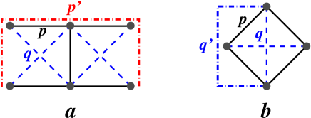
Figure 7: (Color online) a: Illustration of the real-space renormalization-group procedure. The connectivity of a superbond defined by five p- bonds is enhanced by q- bonds, Eq. (59). b: Percolation picture at small $p$. p-bonds ”assist” the connectivity of q- bonds, Eq. (61).

The original approach of Ref. Stenley, applies when $q=0$, i.e., when only p- bonds connecting the sites of $A_{n,m}$ square lattice are present. Within this approach, five p- bonds are replaced by one superbond, as shown with full lines in Fig. 7a. Probability, $p^{\prime}$, that superbond is present, is expressed via probability that p- bond is present, as

$$p^{\prime}\!\! = \!\!P_{5}(p)+P_{4}(p)+P_{3}(p)+P_{2}(p)+P_{1}(p)+P_{0}(p),$$ (53)

$$= \!\!f_{0}(p),$$

where $P_{n}(p)$ is the partial probability that the superbond is present when $n$ original bonds are present. A simple counting of variants yields

$$P_{5}(p)=p^{5},\quad P_{4}=5p^{4}(1-p),\quad P_{3}=8p^{3}(1-p)^{2},$$

$$P_{2}(p)=2p^{2}(1-p)^{3},\quad P_{1}=0,\quad P_{0}=0.$$ (54)

Remarkable feature of the transformation Eq. (53) is that its fixed point, $p^{\prime}=p$, coincides with the exact bond percolation threshold, $p=1/2$, on the square lattice. The q- bonds, shown with dashed lines in Fig. 7. We will incorporate them into renormalization group transformation assuming that their role is the enhancement of connectivity of the superbond. This enhancement occurs differently depending on how many original bonds are present. For example, if all five or four bonds are present, the connectivity of superbond is guaranteed even without any q- bonds, so that $P_{5}$ and $P_{4}$ are not affected by q- bonds. When three p- bonds are present, there are two variants when superbond does not connect. Then the probability that it connects in the presence of q- bonds is given by

$$P_{3}(p,q)=P_{3}(p)+2p^{3}(1-p)^{2}\bigl{[}2q(1-q)+q^{2}\bigr{]}.$$ (55)

The second term is the product of probabilities that p- connectivity is absent and that q- bonds restore it. The factor in the square brackets accounts the fact that restoration can happen by installing one q- bond (two variants) as well as two q- bonds (one variant). The expression for $P_{2}(p,q)$ has a similar structure,

$$P_{2}(p,q)=P_{2}(p)+p^{2}(1-p)^{3}\bigl{[}2\cdot 4\bigr{(}2q(1-q)+q^{2}\bigl{)}\bigr{]}.$$ (56)

Overall, there are ten configurations when two p- bonds of the superbond are present. Out of these ten, there are two variants when the superbond connects; in the remaining eight variants the superbond does not connect. The factor in the square brackets in Eq. (56) describes the probability that in these eight variants q- bonds make the superbond connect. Note that the $q$ dependence of the second term in Eq. (55) is the same as in the case of $P_{2}(p,q)$. This reflects the fact that in both cases installing either one or two q- bonds restore connectivity. If there is only one p- bond, it can be either ”vertical” (one variant) or horizontal (four variants). In the first case, probability of restoring connectivity is a product of the probabilities that it is restored both ”to the left” and ”to the right” from the p- bond. If the p- bond is horizontal, there are three q- bonds that might participate in the restoration of the connectivity. This yields

$$P_{1}(p,q)=p(1-p)^{4}\bigl{[}(2q(1-q)+q^{2}\bigl{)}^{2}$$

$$+4\bigl{(}q(1-q)^{2}+3q^{2}(1-q)+q^{3}\bigr{)}\bigr{]}.$$ (57)

Finally, $P_{0}(p,q)$ is the probability that the superbond connects via q- bonds only. All four q- bonds can participate in restoration, see Fig. 7a. In particular, the connectivity can go through the upper middle site, lower middle site, or both, resulting in

$$P_{0}(p,q)=(1-p)^{5}\bigl{[}2q^{2}(1-q)^{2}+4q^{3}(1-q)+q^{4}\bigr{]}$$ (58)

The net probability that the superbond connects is the sum of $P_{5}(p)+P_{4}(p)$ and Eqs. (55)- (58), namely

$$f(p,q)=f_{0}(p)+2p^{3}(1-p)^{2}\bigl{[}2q-q^{2}\bigr{]}$$ (59)

$$+8p^{2}(1-p)^{3}\bigl{[}2q-q^{2}\bigr{]}$$

$$+p(1-p)^{4}\bigl{[}4q+8q^{2}-8q^{3}+q^{4}\bigr{]}+(1-p)^{5}\bigl{[}2q^{2}-q^{4}\bigr{]}.$$

We determine the line of percolation transitions on the $p,q$- plane upon equating $f(p,q)$ to $\frac{1}{2}$. Solution of this equation is plotted in Fig. 8. At small $q$ the $p(q)$ boundary is linear,

$$p_{c}(q)=\frac{1}{2}-\frac{6}{13}\,q.$$ (60)

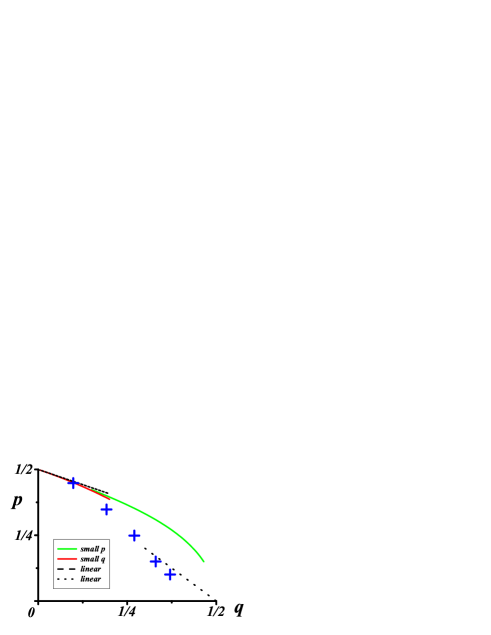
Figure 8: (Color online) The line of percolation transitions in the $(p,q)$-plane is plotted from Eq. (59) for small $q$ (red line) and from Eq. (61) for small $p$ (green line). Dashed and dotted straight lines are the asymptotes, Eq. (60) and Eq. (64) with $\alpha=1$, respectively. Crosses show the positions of quantum delocalization transition inferred from quantum simulations for five values of “energies”, $p$.

In the above procedure we assumed that the effect of q- bonds is a correction to the percolation over p- bonds. Consider now the opposite limit, where $q$ is close to $1/2$ and $p$ is small, so that the percolation is dominated by the q- bonds, while the p- bonds constitute a small correction. First we note that for $p=0$, the regions $A_{n,m}$ with $n+m$ even and $n+m$ odd are decoupled. Moreover, $q=1/2$ corresponds to bond percolation threshold in both decoupled sublattices. Now adding small portion of p- bonds facilitates percolation for $q<1/2$. To describe this facilitation quantitatively we turn to Fig. 7b. This figure illustrates that, instead of one missing q- bond, a pair of one horizontal and one vertical p- bonds can provide the connection, and that there are two such variants. Resulting shift of the threshold position is determined by the condition

$$f(p,q)=q^{\prime}=q+2(1-q^{2})p^{2}=\frac{1}{2},$$ (61)

where $q^{\prime}$ is the renormalized probability that q- bond connects. The origin of the factor $(1-q^{2})$ in Eq. (61) is the following. If the vertical q- bond is missing [with probability $(1-q)$], the two p- bonds which restore connectivity can either share a common site (with probability $2p^{2}$), or two p- bonds can be connected to each other via a horizontal q- bond (with the probability $2p^{2}q$). The sum of probabilities of these two realizations should be multiplied by $(1-q)$. The resulting from Eq. (61) $p(q)$ dependence,

$$p_{c}(q)=\sqrt{\frac{1-2q}{3}}\,,$$ (62)

is plotted in Fig. 8. In fact, as seen from Fig. 8, the asymptotic behaviors found from Eqs. (59) and (61) match very closely near $q=\frac{1}{4}$.

Eq. (61) describes the situation when percolation occurs in one, e.g., $n+m$ even sublattice, while the $n+m$ odd sublattice paly an auxiliary role. This picture is violated near the degeneracy point $p=0$, $q=1/2$. Upon approaching to this point, both sublattices should be treated on the equal footing. Moreover, the position of the boundary on the $p,q$ plane is governed not by a local arrangement of the bonds but rather by large-scale behavior of the clusters in both sublattices. We will discuss percolation transitions in this region in a separate subsection below, after we establish the relation between percolation and electron trajectories in magnetic field.

IV.2 Implication of the percolation transition for transport

The prime question is: to what extent the connectivity of $A_{i,j}$ regions studied in the previous subsection governs the transport over the regions located between the forbidden regions $A_{i,j}$. To emphasize that this question is non-trivial, note that, while p- and q- bonds facilitate the connectivity, a combination of two p-bonds at a given junction and one q- bond through the same junction can give rise to localized electron trajectory, circling around the junction.

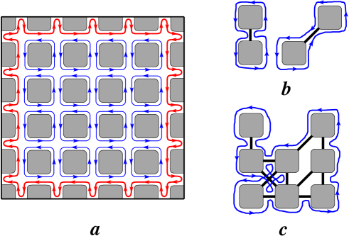
Figure 9: (Color online) a: Structure of electron trajectories at $p=q=0$. Trajectories either encircle forbidden regions, $A_{n,m}$, (brown lines), or constitute a chiral edge state due to reflection from the boundaries (red line). b: Installing one p- (vertical) or q- (diagonal) bond creates a trajectory encircling two forbidden regions counter-clockwise. c: Example of a finite cluster of p- and q- bonds. Formation of trajectory encircling the hull.

To establish the connection between transport and percolation, we start with the simplest case $p=0$, $q=0$. It is apparent from Fig. 5 (see also Fig. 9a) that in this case electron trajectories are closed counter-clockwise loops around forbidden regions $A_{i,j}$. In other words, electron executes counter-clockwise motion along the perimeters of $A_{i,j}$. Now let us switch on a single p- bond, say, between $A_{n,m}$ and $A_{n,m-1}$, Fig. 9b. It is easy to see that installing this bond creates a closed trajectory encircling two regions, joined by the bond, in such a way that the forbidden joined region remains on the left. Thus, from two trajectories along the perimeters of disconnected regions we get one trajectory along the perimeter of the joined region Fig. 9b. The same happens upon installing a single q- bond, as shown in Fig. 9b. In fact, this evolution is general: if a portion of p- and q- bonds connect several forbidden regions into a cluster, there appears a closed trajectory along outer perimeter of the cluster. While moving along this perimeter trajectory, the cluster remains on the left. For the transport properties of p-q model, the outer perimeter, which signifies the most delocalized trajectory existing with the given cluster, plays a central role. Note that in the percolation theory such a perimeter is called a hull. Thus we see that hulls of the bond percolation Fig. 9c correspond to the most important electron trajectories of the p-q model, in the sense, that, upon approaching the percolation threshold, the hulls of big clusters join into even bigger hulls. Extent of the region available for electron motion is determined by the size of the typical cluster, which is the localization radius of the classical percolation. While locally the motion occurs along the boundaries of forbidden regions $A_{i,j}$, at large scales the hulls define the extent of the motion. Now we can identify the point of the percolation threshold at which $A_{i,j}$ get connected into infinite cluster with the point when the hull trajectories become infinite and connect opposite sides of macroscopic sample.

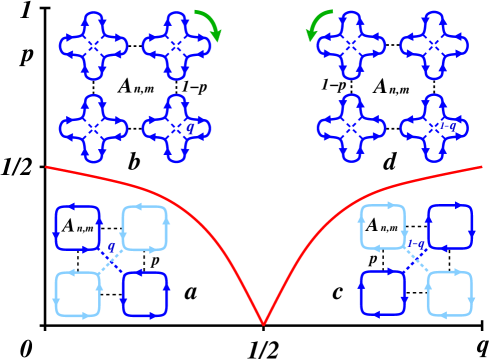
Figure 10: (Color online) Phase diagram (red line) of the p-q model in the regime of strong disorder. Phases (a) and (c): electron predominantly encircles forbidden regions $A_{n,m}$, moving counter-clockwise (a) or clockwise (c). Coupling of neighboring forbidden regions via p- and q- bonds is weak. Phases (b) and (d): electron predominantly encircles nodes, moving counter-clockwise (d) or clockwise (b). Coupling of nodes due to absent p- bonds is weak. Edge trajectory disappears upon crossing the boundary (red line), (a) $\rightarrow$ (b) or (c) $\rightarrow$ (d).

Essentially, hulls can provide a connectivity through an infinite sample exactly at the percolation threshold. Below and above this threshold, hulls either do not provide a macroscopic connectivity or establish a trajectory extending along the macroscopic edges of a sample, depending on boundary conditions. Being translated into the p-q model transport properties, this means that a non-zero diagonal conductivity, $\sigma_{xx}\neq 0$, is possible only at the percolation transition, which separates two insulating regimes with $\sigma_{xx}=0$.

We now choose the boundaries of the macroscopic p-q sample passing through the centers of the end regions $A_{i,j}$, as shown in Fig. 9a, and assume full reflection at the boundaries. It can be seen that for $p=0$, $q=0$, there is a macroscopic trajectory spanning near the edges around the sample in the clockwise direction. Therefore, in the phase $a$, Fig. 10, we have nonzero $\sigma_{xy}$, while $\sigma_{xx}=0$ because there is no trajectory through the sample at $p=q=0$ and in the vicinity.

Previous consideration pertains to small enough $p$ and $q$. Let us now move along the boundary $q=0$. In the absence of q- bonds this corresponds to increasing connectivity, $p$, in conventional bond percolation problem. It is easy to see that the edge state disappears when we pass the percolation threshold $p=1/2$. Above this point, the electron trajectories are strongly localized around the junctions (phase $b$ in Fig. 10), and describe the clockwise motion, unlike counter-clockwise loops in the phase $a$.

Now we fix $p$ in the domain $(1-p)\ll 1$ and move along the q- axis. At this point we note that the p-q model possesses a duality $q\rightarrow(1-q)$. One transparent way to reveal this duality is to trace the change in strongly localized trajectories, phase $b$, upon changing $q$ by $(1-q)$. One can see that trajectories remain unchanged, while the direction changes from counterclockwise to clockwise. Such a change could be expected on purely physical grounds, since transformation $q\rightarrow(1-q)$ means that the difference, $(1/2-q)$, which represents magnetic field, changes sign. Naturally, reversal of magnetic field results in the change of direction in which the $A_{n,m}$ regions are circumvented. Therefore there is one-to-one correspondence between the strongly localized phase $b$ and phase $d$. The same argument, change of direction of the rotation as a result of $q\rightarrow(1-q)$ transformation, suggests that the phase $c$ is mirror image of the phase $a$, with the opposite sign of $\sigma_{xy}$.

IV.3 Vicinity of the degeneracy point $p=0$, $q=1/2$

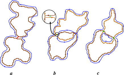
Figure 11: (Color online) Vicinity of the point $p=0$, $q=1/2$, of the phase diagram Fig. 10. a: Two q-clusters on the same sublattice hybridize upon installing a q- bond. b: A q- cluster of $n+m$ odd sublattice (upper) and a q- cluster of $n+m$ even sublattice (lower) overlap. A joined trajectory (thin blue line) is formed upon installing of a single p- bond. The blowup illustrates hybridization of trajectories on a microscopic level. c: Same as (b), but with two p- bonds connecting q- clusters. Blue lines illustrate that the hull trajectory and ”internal” trajectory are disconnected.

In the close vicinity, $(1/2-q)\ll 1$, $p\ll 1$, of the degeneracy point, one has big clusters of q- bonds in $(n+m)$ even and $(n+m)$ odd sublattices, which are statistically equivalent. Let us start our consideration from some $q=q_{0}<1/2$ and $p=0$. Connectivity via q- bonds can be enhanced either by adding p- bonds or by shifting $q$ closer to $1/2$. We argue that, close enough to the degeneracy point, both operations are equivalent. This is because the number of ”even” q- bonds, i.e., the q-bonds from the $(n+m)$-even sublattice, and the number of ”odd” q- bonds, i.e., the q-bonds from the $(n+m)$-odd sublattice, involved in a typical cluster, is the same. Once this ”equal participation” of two sublattices is achieved, it is preserved upon increasing both $p$ and $q$. The value of $p$ necessary to achieve this equal-participation regime obviously depends on proximity of $q$ to $1/2$. A way to estimate this necessary $p$ is based on the following reasoning. The spatial separation between neighboring p- bonds is $\sim 1/\sqrt{p}$. If this separation is smaller than the typical size of q- cluster, $\sim|1/2-q|^{-4/3}$, on a given sublattice, i.e.,

$$p>\left(\frac{1}{2}-q\right)^{8/3},$$ (63)

then p- bonds connect clusters from different subnetworks. The way in which equal-participation regime sets in is illustrated in Fig. 11. In Fig. 11a the condition Eq. (63) is not met; clusters grow independently in each sublattice as $q$ increases. Figs. 11b,c illustrate that a typical clusters on one sublattices is overlapped by some other typical cluster from another sublattice. Therefore, few p- bonds per cluster, see Eq. (63), are sufficient for formation of a unified cluster. Percolation boundary, $p_{c}(q)$, lies above the boundary of equal-participation regime Eq. (63). It is reasonable to assume that the percolation threshold corresponds to certain portion of p- and q- bonds per site. Having in mind that in equal-participation regime p- and q- bonds are equivalent within a factor, the above assumption leads us to

$$p_{c}(q)\simeq\alpha{\Big{|}}\frac{1}{2}-q{\Big{|}},$$ (64)

with numerical coefficient, $\alpha\sim 1$. This linear behavior, as well as the forms Eqs. (60) and (62), are in agreement with the condition Eq. (63), which in fact should hold in the whole domain where we expect delocalization transitions with the participation of p- bonds. The above reasoning, leading to the linear boundary Eq. (64) is by no means rigorous. We were able to come up with more compelling reasoning that for the case when half of q- bonds are replaced by $1-q$, the percolation transition at small $p$ indeed occurs at $p\sim(1/2-q)$. Note however, that one cannot claim that this auxiliary problem provides evidence for linear boundary in our p-q model. This is because approaching the point $(p,q)=(0,1/2)$, can depend of the direction of the approach, so that the approach along a path with ”balanced” $q$ and $1-q$ bond can yield a different boundary.

Moreover, this linear dependence is a source of an apparent doubling of the critical exponent when one approaches the delocalization point along the horizontal line $p=\text{const}\ll 1$.

IV.4 Doubling of the critical exponent

The shape of the percolation transition line Eq. (64) for which the condition Eq. (63) is met, allows one to make quantitative predictions about the behavior of the localization radius, $\xi(p,q)$. The reasoning goes as follows. Eq. (63) ensures that the typical clusters on the two sublattices with sizes $\xi(q)$ are connected by p- bonds. Now, if we keep $q$ unchanged and approach the critical line, $p_{c}(q)$, from below, the localization radius grows as

$$\xi(p,q)\sim\frac{\xi(q)}{\bigl{[}p_{c}(q)-p\bigr{]}^{4/3}}.$$ (65)

While this relation is asymptotically exact near the delocalization line, we assume that it still holds deeper into the region (a), Fig. 10. Then, in order to find an explicit dependence $\xi(p,q)$, Eq. (64) can be used in Eq. (65), yielding

$$\xi(p,q)\sim\frac{\xi(q)}{\left[\alpha\left(\frac{1}{2}-q\right)-p\right]^{4/3}}.$$ (66)

Note now that Eq. (66) can be interpreted as a doubling of the critical exponent. As one starts at some point, $(p_{0},q)$, such that $p_{0}\ll 1$ and $(1/2-q)\sim 1$ and move towards the transition boundary along the horizontal line $p=p_{0}$, localization radius changes as follows

$$\xi(p_{0},q){\Big{|}}_{q<1/2}\sim\frac{1}{\left[\frac{1}{2}-q\right]^{4/3}\left[\frac{1}{2}-\frac{p_{0}}{\alpha}-q\right]^{4/3}}.$$ (67)

For $(1/2-q)\gg p_{0}/\alpha$ Eq. (67) assumes the form

$$\xi(p_{0},q)\sim\frac{1}{\left[\frac{1}{2}-q\right]^{8/3}},$$ (68)

which means that the subcritical behavior of $\xi(p_{0},q)$ as a function of $q$ is similar to the usual $|q-q_{c}|^{-4/3}$, but with the doubled critical exponent. Therefore, it is the linear behavior Eq. (64) which leads to the doubling. On the other hand, as we have reasoned in the previous subsection, the linearity of the boundary of the percolation transition is a consequence of the ”interaction” of two subnetworks.

The remaining question is the behavior of $\xi(p,q)$ along the line $q=1/2$. To address this question, note that there are two delocalization transitions which take place as $q$ is changed along the line $p=p_{0}\ll 1$; the first one at $q=q_{c1}<1/2$ and the second at $q=q_{c2}>1/2$. By virtue of duality, $q_{c1}$ and $q_{c2}$ are related as $q_{c1}+q_{c2}=1$. For small $p$, from Eq. (64) we have

$$q_{c1}(p)=\frac{1}{2}-\frac{p}{\alpha},\qquad q_{c2}(p)=\frac{1}{2}+\frac{p}{\alpha}.$$ (69)

In the domain $q>1/2$ the $\xi(p,q)$ dependence can be found using the above arguments

$$\xi(p_{0},q){\Big{|}}_{q>1/2}\sim\frac{1}{\left[q-\frac{1}{2}\right]^{4/3}\left[q-\frac{1}{2}-\frac{p_{0}}{\alpha}\right]^{4/3}}.$$ (70)

Recall that in Eq. (67), the factor $[1/2-q]^{-4/3}$ appears as a length of the unit plaquette in the percolation over p-bonds. Then the second factor, $[1/2-p_{0}/\alpha-q]^{-4/3}$, can be regarded as a localization radius associated with the delocalization transition at $q_{c1}(p_{0})$. The general expression which respects the duality and contains as limits Eqs. (67) and (70) reads

$$\xi(p,q)\sim\frac{1}{{\big{|}}\frac{1}{2}-\frac{p}{\alpha}-q{\big{|}}^{4/3}{\big{|}}\frac{1}{2}+\frac{p}{\alpha}-q{\big{|}}^{4/3}}.$$ (71)

In particular, along the line $q=1/2$ this expression predicts the following behavior of localization radius

$$\xi(p){\Big{|}}_{q=1/2}\propto\frac{1}{p^{\,8/3}}.$$ (72)

IV.5 Consequences of the doubling

Below we will demonstrate numerically that Eq. (71) applies also to the quantum delocalization upon replacement $4/3$ by the quantum critical exponent of localization radius. Here we would like to emphasize the similarity between the quantum version of Eq. (71) and energy dependence of the localization radius in the case of close, e.g., spin-split delocalized states in strong magnetic field. Behavior of $\xi$, similar to Eq. (71), was conjectured in Ref. Doubling, and demonstrated numerically in Refs. LeeChalker94, ; LeeChalkerKo94, . In our case, two close delocalized states correspond to opposite directions of magnetic field, and thus have opposite chiralities. On the contrary, in Refs. Doubling, ; LeeChalker94, ; LeeChalkerKo94, ; hanna95, , chiralities of both delocalized states, which are close in energy, are the same. More microscopic demonstration of doubling in the system with two close in energy delocalized states with the same chirality can be found in Ref. Gramada97, . The situation considered in Ref. Gramada97, was two layers with smooth random potential coupled by tunneling with amplitude, $t_{0}$. For a single layer, the transmission of a saddle point is given by $T(E/\Gamma)=[1+\exp(E/\Gamma)]^{-1}$. For two layers, tunneling allows to bypass saddle points. Instead, the role of a saddle point is played by the region where equipotentials from different layers come close to each other, but do not intersect. It was demonstrated in Ref. Gramada97, that for $E$ outside the interval $(-t_{0},t_{0})$ the transmission of such an effective saddle point is given by $\tilde{T}(E/\tilde{\Gamma})=T(E^{2}/\tilde{\Gamma}^{2})$, where $\tilde{\Gamma}$ depends on $t_{0}$ as $t_{0}^{1/4}$. Therefor, while in the vicinity of delocalized states $E=\pm t_{0}$ the critical behavior of localization length is $\xi\propto|E\pm t_{0}|^{-\nu}$, outside the interval $(-t_{0},t_{0})$ we have $\xi\propto(E^{2})^{-\nu}$, which mimics the doubling of the critical exponent.

IV.6 Physical interpretation of the phase diagram Fig. 10

In physical terms, the p-q boundary in Fig. 10 relates the backscattering probability, $p$, and magnetic filed, $(1/2-q)$, at which delocalization transition takes place. The parameter $p$ can be viewed as a measure of disorder and also as a measure of electron energy, $E_{\scriptscriptstyle F}$; obviously, $p$ decreases monotonously with increasing $E_{\scriptscriptstyle F}$. Then, the domain $q<1/2$ of the phase boundary in Fig. 10 translates into the low-field region, $\omega_{c}\tau<1$, of the dependence $E_{0}(\omega_{c})$ in Fig. 1. Correspondingly, the domain $q>1/2$ maps onto $E_{0}(\omega_{c})$ dependence with reversed sign of the magnetic field. More detailed correspondence between Figs. 1 and 10 can be established upon identification of $\sigma_{xy}$ values for different phases. As we demonstrated above using percolation language, there is no edge state in the central phase, which includes regions $b$ and $d$ in Fig. 10. Since this phase represents the region $E_{\scriptscriptstyle F}<E_{0}(\omega_{c})$ in Fig. 1, this phase should be identified with the Anderson insulator. We have also demonstrated, see Fig. 9a, that there is one chiral edge state in the phase $a$ of the phase diagram. Thus, in the region $E_{\scriptscriptstyle F}>E_{0}(\omega_{c})$ in Fig. 1 we have $\sigma_{xy}=1$, so this phase is a quantum Hall insulator. In the region $p>1/2$ there are no delocalized states in Fig. 10. This region translates into the strongly localized regime, $E_{\scriptscriptstyle F}<1/\tau$, i.e., below the minimum of the $E_{0}(\omega_{c})$ curve.

Linearity of the $p_{c}(q)$ boundary can be rewritten in terms of observables. Upon identifying $p$ with $1/(k_{F}l)$ and $(1/2-q)$ with $\omega_{c}\tau$, the position of the boundary can be presented as $(k_{F}l)(\omega_{c}\tau)=\text{const}$. This quantifies the levitation rate, $\omega_{c}\tau\propto 1/(k_{F}l)$. Curiously, it coincides with the prediction of scaling theory, Eq. (8).

For conclusive confirmation of the levitation scenario it should be demonstrated that the p-q phase boundary retains its shape in the presence of quantum interference. In fact, the quantum and ”percolation” boundaries almost coincide. The evidence for that will be presented in the next Section.

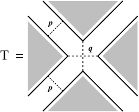
Figure 12: Illustration of the transfer matrix, T, Eq. (73), of the p-q model. Two q- bonds correspond to the first matrix in the product Eq. (73); two p- bonds correspond to the third block-diagonal matrix in the product.

V Numerical results for quantum delocalization

V.1 Transfer matrix

Scattering matrices on the links and at the nodes are given by Eqs. (32) and (48), respectively. With regard to numerical simulations, the p-q model is quite similar to the models with mixing of two co-propagating channels on the links, studied in Refs. Kagalovsky95, ; kagalovsky97, ; LeeChalker94, ; LeeChalkerKo94, .

The transfer matrix, T, at each node of the network is a $4\times 4$ matrix, which transforms four amplitudes on the left into four amplitudes on the right. We incorporate the link p-matrices and junction q-matrices into T in the way illustrated in Fig. 12. It follows from Fig. 12 that T matrix can be parameterized as

$$\text{\large T}=\!\left(\!\!\begin{array}[]{cccc}{\scriptstyle\frac{1}{\sqrt{1-q}}}&0&0&{\scriptstyle\sqrt{\frac{q}{1-q}}}\\ 0&{\scriptstyle\frac{1}{\sqrt{q}}}&{\scriptstyle\sqrt{\frac{1-q}{q}}}&0\\ 0&{\scriptstyle\sqrt{\frac{1-q}{q}}}&{\scriptstyle\frac{1}{\sqrt{q}}}&0\\ {\scriptstyle\sqrt{\frac{q}{1-q}}}&0&0&{\scriptstyle\frac{1}{\sqrt{1-q}}}\end{array}\right)\!\!\!\left(\!\!\begin{array}[]{cccc}e^{i\varphi_{1}}&0&0&0\\ 0&e^{i\varphi_{2}}&0&0\\ 0&0&e^{i\varphi_{3}}&0\\ 0&0&0&e^{i\varphi_{4}}\end{array}\!\!\right)\!\!\left(\!\!\begin{array}[]{cccc}{\scriptstyle\frac{1}{\sqrt{1-p}}}&{\scriptstyle\sqrt{\frac{p}{1-p}}}&0&0\\ {\scriptstyle\sqrt{\frac{p}{1-p}}}&{\scriptstyle\frac{1}{\sqrt{1-p}}}&0&0\\ 0&0&{\scriptstyle\frac{1}{\sqrt{1-p}}}&{\scriptstyle\sqrt{\frac{p}{1-p}}}\\ 0&0&{\scriptstyle\sqrt{\frac{p}{1-p}}}&{\scriptstyle\frac{1}{\sqrt{1-p}}}\end{array}\!\!\right)\!\!\!\left(\!\!\begin{array}[]{cccc}e^{i\phi_{1}}&0&0&0\\ 0&e^{i\phi_{2}}&0&0\\ 0&0&e^{i\phi_{3}}&0\\ 0&0&0&e^{i\phi_{4}}\end{array}\!\!\right).$$ (73)

The second and the fourth matrices in the product describe random phases acquired between the point contact and the junction.

Once the transfer matrix is specified, one can find the transfer matrix of a slice with $M$ nodes in transverse direction. As usual, to study the critical properties, numerical simulations are performed on a system with fixed width $M=2^{k}$, then repeated for $4$,$5$, $6$, $7$ and sometimes even $k=8$. By multiplying transfer matrices for a stripe with $N$ slices and diagonalizing the resulting total transfer matrix, it is possible to extract the smallest positive Lyapunov exponent $\lambda_{M/2}$ (the eigenvalues of the transfer matrix are $\exp(\lambda_{i}N)$). The localization length, $\xi_{M}$, is proportional to $1/\lambda_{M/2}$. The state is identified as a critical one when the renormalized localization length, $\xi_{M}/M$, becomes independent of the system width, $M$. We consider this as a criterion for a transition point, that determines the value $q=q_{c}$, for a fixed value of $p$. Practically, $q=q_{c}$ emerges as a maximum in $\xi_{M}/M$ vs. $q$ for large system widths, when finite-size errors become small.

Close to $q=q_{c}$, the ratios $\xi_{M}/M$ should satisfy a one-parameter scaling

$$\frac{\xi_{M}}{M}=f\left(\frac{\xi(q)}{M}\right),$$ (74)

which is commonly used to infer the localization length, $\xi$.

We first check that our numerical data support Eq. (74); to do so we fit all the data points onto one curve according to Eq. (74). The fit is carried out with the help of a special optimization program. This optimization program runs different critical $q$-values and critical exponents $\nu$ and chooses the optimal sets, $q_{c}$ and $\nu$, which provides the best agreement with Eq. (74).

We now briefly describe the optimization procedure. The routine determines least-squares polynomial approximation by minimizing the sum of squares of the deviations of the data points from the corresponding values of a polynomial. The argument of the function fitted by the Chebyshev polynomials is $M|q-q_{c}|^{\nu}$. To choose the optimal pair, $q_{c}$ and $\nu$, we run this routine for the wide range of values $q_{c}$ and $\nu$. For most of the points on the critical line the values of $q_{c}$, obtained by two methods: (i) searching for $q$ at which $\xi_{M}/M$ is constant and (ii) using optimization procedure, agree with each other.

Note however, that in two limiting cases, $p\rightarrow 0$ and $p\rightarrow 1/2$, where the data strongly fluctuate, apparent discrepancies arise. For very small values of $p$ the off-diagonal terms in the transfer matrix are close to $0$ (they are $\sim\sqrt{p}$), leading to strong fluctuations in numerical results. Physically, enhancement of fluctuations near $p=0$ is a result of proximity to two critical points, $q_{c}$ and $1-q_{c}$, see Fig. 10, where the doubling of critical exponent takes place. On the other hand, when $p$ is close to $1/2$, we have $q_{c}$ close to $0$. Strong fluctuations in the data in this case is a consequence of small denominators, $1/\sqrt{q}$, in the transfer matrix Eq. (73). Altogether, both methods yield close values of $q_{c}(p)$.

The last remark on simulation procedure is on the boundary conditions in transverse direction. In CC model, the periodic boundary conditions in transverse direction are insured upon imposing requirement on the structure of transfer matrix of even slices only. The same is true for the p-q model. Unlike the CC model, where the reflection and transmission at the nodes alternate between subsequent slices, the elementary transfer matrices in the p-q model, Eq. (73), are the same for even and odd slices. This equivalence is a result of symmetry of a single node with respect to $90^{\circ}$ rotations in the p-q model.

V.2 Zero magnetic field

Zero magnetic field corresponds to the line $q=1/2$ on the $p,q$ plane. Above we identified this line with the vertical energy axis in Fig. 1. Since the key ingredient of the levitation scenario is that all the states on this axis are localized, we start with studying localization properties along the line $q=1/2$.

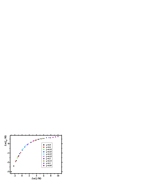
Figure 13: (Color online) A fit of $\xi_{M}/M$ data points for the p-q model at $q=1/2$ to a one-parameter scaling form: $\ln\left(\xi_{M}/M\right)$ vs. $\ln\left(\xi/M\right)$.

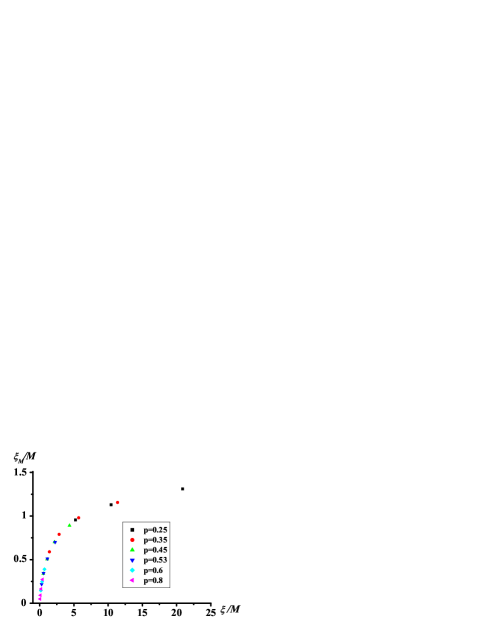
Figure 14: (Color online) One parameter scaling function, $\xi_{M}/M=f(\xi/M)$, is plotted from Fig. 13.

To obtain a scaling plot, $\xi_{M}/M=f(\xi(p)/M)$, we analyzed 40 data points: four $M$-values, $M=16,\,32,\,64,\,128$, and ten $p$-values, $p=0.05,\,0.1,\,0.15,\,0.2,\,0.25,\,0.35,\,0.45,\,0.53,\,0.6,\,0.8$. By plotting $\ln\left(\xi_{M}/M\right)$ vs. $-\ln M$ and shifting points for different $p$ to fall on the same line, we get the result shown in Fig. 13. It is seen that the quality of scaling is high. The scaling function, $f$, found from the data in Fig. 13, is shown in Fig. 14. The dependence, $\xi(p)$ inferred in this way is plotted in Fig. 15 with the black line. Our result confirms the expectation that the localization length in zero magnetic field increases rapidly even in log-scale as $p$ goes to zero. Scaling theory predicts the dependence, $\ln\xi_{u}\sim(k_{\scriptscriptstyle F}l)^{2}$, Eq. (3). Since we have earlier identified $k_{\scriptscriptstyle F}l$ with $1/p$, we expect the dependence, $\ln\xi(p)\sim 1/p^{2}$. The black curve in Fig. 15 falls off with $p$ slower, and can be well approximated with $\ln\xi(p)=0.99-4\ln p$. One possibility to account for this discrepancy is that asymptotic $1/p^{2}$ behavior is achieved at $p$ smaller that $0.05$- the minimal $p$ we studied. Note however that the total range of change of $\xi(p)$ in the domain we studied is huge: $\xi(0.05)/\xi(0.8)\approx 5.5\times 10^{4}$.

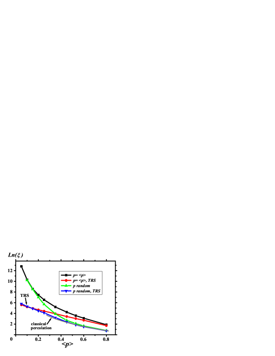
Figure 15: (Color online) Localization radius of the p-q model in a zero magnetic field ($q=1/2$) is plotted vs. inverse ”energy”, $\langle p\rangle$ for the cases: no spread in scattering strengths on the links, $p=\langle p\rangle$, and no TRS on the links (black), $p=\langle p\rangle$, with TRS on the links (red). Blue and green curves show $\ln\xi$ with and without TRS, respectively, plotted for the strong disorder in scattering strengths on the links: $p$ randomly assumes the values $0.01$ and $0.99$ while the inverse ”energy” is the average value, $\langle p\rangle$. Grey curve [$\ln(\xi/\xi_{0})=-\frac{8}{3}\ln p$] is the result of the percolation treatment Eq. (72). The constant $\xi_{0}$ is chosen to match the data at $\langle p\rangle=0.8$.

Another prediction of the scaling theory is that the presence of time reversal symmetry (TRS) the growth of localization radius with $k_{\scriptscriptstyle F}l$ is much slower, $\ln\xi_{o}\sim k_{\scriptscriptstyle F}l$, Eq. (2). In the above simulations we assumed that magnetic field is zero in the ”orbital” sense ($q=1/2$), but phases on the links were ”unitary”. This is because the orthogonal-unitary crossover takes place at exponentially small $(1/2-q)$. However, in order to relate closer our calculation to the scaling theory, we ran simulations with TRS on the links restored. This amounts to setting $\varphi_{2}=-\varphi_{1}$, $\varphi_{4}=-\varphi_{3}$, $\phi_{2}=-\phi_{1}$, and $\phi_{4}=-\phi_{3}$ in Eq. (73). The scaling function obtained with TRS is shown in Fig. 16, and the corresponding $\xi(p)$ is plotted in Fig. 15 with the red curve. As could be expected, in the strongly localized domain, $p>0.6$, there is no difference between the unitary and orthogonal cases. Upon decreasing $p$, orthogonal $\xi(p)$ indeed grows much slower than unitary $\xi(p)$, so that $\xi(0.05)/\xi(0.8)\approx 48.5$. The fact that orthogonal $\ln\xi(p)$ extrapolates at $p\rightarrow 0$ to a finite value also suggests that diverging behavior sets in at $p$ smaller than $0.05$.

In the above analytical treatment of the p-q model we considered the limit of strong disorder, which is a strong spread in the local values of $p$ with average $p=\langle p\rangle$ fixed. Consideration was based on the understanding that strong spread in $p$ eliminates completely the interference effects, and thus reduces the analysis of the p-q model to the percolation problem, which predicts much smaller localization radius, $\xi(p)\sim 1/p^{8/3}$, Eq. (72). In order to test this expectation, we incorporated a strong spread in $p$ into transfer-matrix calculation. Namely, for a fixed $\langle p\rangle$ we randomly set the values $p=0.01$ or $p=0.99$ on each link. Our results on $\xi(p)$ with and without TRS are shown in Fig. 15 with the blue and green lines, respectively. We see that our expectation is confirmed within the region $p>0.5$. In this region, the two curves with disorder are not sensitive to universality class and are well below the curves without disorder in $p$. Moreover, their behavior in this region is in accord with prediction of percolation theory. Indeed, percolation theory predicts $\xi(0.53)/\xi(0.8)=(0.8/0.53)^{8/3}\approx 3$. From the blue and green curves we get the close values, $3$ and $3.67$, respectively. Fig. 15 also illustrates that for $p<0.5$, quantum mechanics ”wins” over disorder: the curves with random $p$ merge with curves without disorder in $p$ corresponding to their respective symmetry classes.

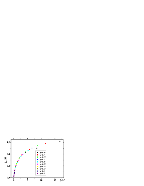
Figure 16: (Color online) A fit of $\xi_{M}/M$ data points for the p-q model at $q=1/2$ with time reversal symmetry on the links to a one-parameter scaling form $\xi_{M}/M=f(\xi/M)$.

The above results pose an acute question: whether the boundary, $p_{c}(q)$, of delocalization transitions, which was established within the percolation treatment, and extends in the region $p<0.5$, is preserved in fully quantum limit. A related question is whether this boundary is sensitive to the universality class. We address these questions below.

V.3 The line of delocalization transitions and critical exponent

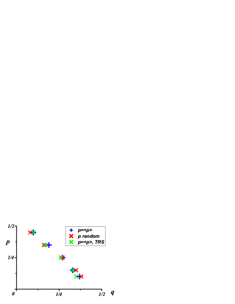
Figure 17: (Color online) Delocalization points for three different sets of $p$: non-random $p$, random $p$ with given $\langle p\rangle$, and non-random $p$ with the TRS.

Our main result, $p_{c}(q)$ boundary without TRS, is shown in Fig. 8 with crosses. Five points obtained for $p=0.1$, $0.15$, $0.25$, $0.35$, and $0.45$, essentially fall onto a straight line, $p=1/2-q$. Deviation from this line takes place near $p=1/2$, where the data-points match well the results of percolation treatment (red line). This confirms our expectation that percolation treatment of the p-q model correctly predicts position of the quantum delocalization transition. Certainly, the critical exponent of delocalization transition is different: $\nu=7/3$ instead of $\nu=4/3$ for percolation. For smaller $p$, deviation from the percolation treatment (green line) is notable. On the other hand, as we explained above, our percolation estimate is rather rude at small $p$. We also argued that the true small-$p$ percolation boundary should be linear. This linearity would mean that the constant, $\alpha$, in Eq. (64) is $\alpha=1$.

More numerical results for p-q boundary are presented in Fig. 17. For comparison, we reproduced the blue crosses from Fig. 8 in Fig. 17. Red crosses demonstrate that the boundary is robust against strong disorder in backscattering strength, $p$. In the same way as for zero magnetic field, the disorder in $p$ was incorporated by randomly choosing local values of $p$ to be $0.99$ or $0.01$ while keeping $\langle p\rangle$ fixed. Coincidence of the two boundaries indicates that delocalization transition is governed exclusively by average $p$, but does not depend on local disorder.

The fact that in the CC model the position of the delocalized state does not depend on the spread in local transmission coefficients of the nodes (i.e., the spread in saddle point heights), is obvious consequence of duality. On the other hand, the p-q model does not possess duality, so that coincidence of the two boundaries is by no means obvious. It can be interpreted as an evidence that, even in magnetic field, localization properties of the system are governed by zero-field conductance, $\sim 1/\langle p\rangle$.

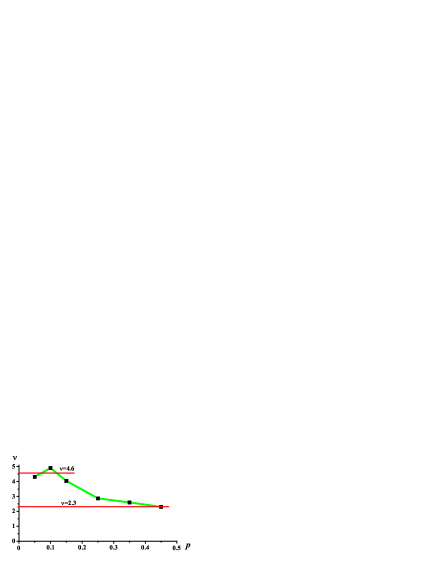
Figure 18: (Color online) Dependence of the critical exponent $\nu$ on $p$ as inferred from optimization procedure, described in the text. As $p$ decreases from $1/2$ to $0$, $\,\nu(p)$ grows approximately twice.

Change of the universality class amounts to replacement $1/\sigma_{xx}$ (unitary) by a constant (orthogonal) in the first term of the scaling equation Eq. (5). If the scaling theory applies, this replacement should not affect the fixed point, $\sigma_{xy}=n$. In other words, only orbital action of magnetic field is sufficient to drive the system into quantum Hall insulator state footnote . We were able to check this prediction within the p-q model. Green crosses in Fig. 17 show the position of p-q boundary with TRS. Overall, the boundaries with and without TRS coincide. Discrepancy at $p=0.1$ is likely due to strong fluctuations of the data at small $p$.

Together with p-q boundary, optimization procedure produced the value of critical exponent, $\nu$. The dependence $\nu(p)$ is shown in Fig. 18. Horizontal lines in Fig. 18 are drawn to illustrate that simulations indicate apparent doubling of the critical exponent, discussed for classical percolation in the previous section. As follows from this discussion, the doubling, revealed by numerics, is a consequence of two close delocalized states. If scaling analysis could be carried our in the immediate vicinity of a given delocalized state, it would recover the conventional value, $\nu\approx 7/3$. Indeed, for $p=0.45$, where two delocalized states are far apart, optimization yields $\nu(0.45)=2.3$, while for $p=0.1$, where the fluctuations are strong, we get $\nu(0.1)=4.9$, which is even bigger than $2\cdot 7/3$. What is remarkable about Fig. 18 is that the apparent growth of $\nu$ upon decreasing $p$ starts quite early, e.g., for $p=0.25$ we get $\nu=2.9$. To make sure that optimization does not distort the raw data, we have checked the scaling manually and reproduced the largest and smallest values of $\nu$.

VI Triangular p-q model

In the previous consideration, electron motion was restricted to the channels between forbidden regions, $A_{n,m}$, with centers residing on a square lattice. This consideration led us to the phase diagram Fig. 8, containing the line of delocalization transition in the $p,q$- plane. In the present section we will demonstrate that the same shape of the transition line emerges when the centers of the forbidden regions constitute a hexagonal lattice, as shown in Fig. 19. This figure illustrates that, similarly to the square p-q model, backscattering takes place on the links. Fig. 19 also illustrates that for hexagonal arrangement of forbidden regions, a junction corresponds to the point where six such regions come close.

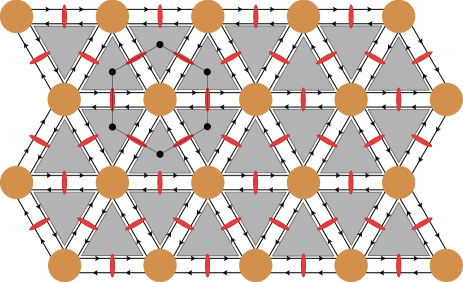
Figure 19: (Color online) Triangular version of the ”square” p-q model, Fig. 5. Point contacts on the links stand for the same $2\times 2$ scattering matrix as in Fig. 5, while the bend-junctions are described by a $6\times 6$ matrix Eq. (113). The centers of the forbidden regions (shaded triangles) constitute a hexagonal lattice.

By contrast to the square p-q model, a wave incident on a junction can be scattered not into two but rather into three directions. Namely, it can proceed forward, or get deflected by the angles $\pm\pi/3$, Fig. 19. Recall that for the square p-q model the $4\times 4$ scattering matrix of a junction Eq. (48) had a simple form, namely, a direct product of two $2\times 2$ matrices. Correspondingly, the $6\times 6$ junction scattering matrix in Fig. 19 is a direct sum of two $3\times 3$ matrices [see Eq. (113) below]. This is a consequence of the fact that the two channels on a given link are not mixed by the junction. As a result, similarly to the square p-q model, upon switching off the backscattering on the links, the network breaks into two decoupled fully chiral networks. While for the square p-q model each chiral network was of CC type, here each chiral network represents a ”triangular” model introduced in Ref. Triangular, . This chiral model, illustrated in Fig. 20, is called triangular because the nodes are arranged on a triangular lattice. For convenience, we briefly review the triangular network model Ref. Triangular, in the next subsection.

VI.1 Fully chiral triangular model

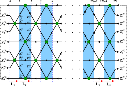
Figure 20: (Color online) A slice of triangular network of width $M=8$ is shown. Three amplitudes on the links to left of green dot are related to three amplitudes to the right of green dot via matrix $\mathbf{X}$. The upper and the lower boundaries of the slice are connected by dashed-dotted lines manifesting that the amplitudes on these boundaries are the same by virtue of cyclic boundary conditions. Upon passing the white stripe, the vector of the amplitudes $\{Z_{i}\}$ is multiplied by the matrix $\mathbf{L}_{1}$. Upon passing the blue stripe the vector $\{\tilde{Z}_{i}\}$ is multiplied by $\mathbf{L}_{2}$.

Microscopic picture underlying CC and triangular chiral models is illustrated in Fig. 21. Fully chiral motion represents drift of the Larmour circle along equipotential lines of smooth random potential. In CC model equipotentials meet pairwise at the saddle points. As the energy, $\varepsilon$, passes through zero, the geometry of equipotentials evolves from reflection to transmission, as shown in Fig. 21a. The scattering matrix describing this evolution near $\varepsilon=0$ has the form CC

$$S_{cc}(\varepsilon)=\left(\begin{array}[]{cc}\,\frac{1}{\sqrt{2}}+\varepsilon&\frac{1}{\sqrt{2}}-\varepsilon\\ \\ -\frac{1}{\sqrt{2}}+\varepsilon&\frac{1}{\sqrt{2}}+\varepsilon\\ \end{array}\right).$$ (78)

At $\varepsilon=0$ the power reflection and transmission coefficients are both equal to $1/2$.

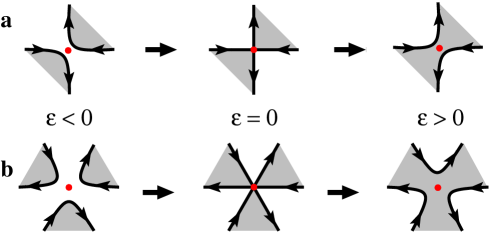
Figure 21: (Color online) Evolution of the equipotential lines: (a) in the CC model, (b) in the chiral triangular model.

In triangular model it is assumed that smooth potential has $120^{\circ}$ rotational symmetry. As a result, equipotentials meet in the groups of three. As $\varepsilon$ is swept through zero, they evolve from reflection (shaded regions disconnected) to transmission (shaded regions fully connected), see Fig. 21b. Near $\varepsilon=0$, probabilities of scattering to the left, to the right and forward, are all finite. Obviously, at $\varepsilon=0$ probabilities of the left- and right- scattering are equal to each other. In Ref. Triangular, it was demonstrated that these probabilities are equal to $4/9$. Correspondingly, the probability of the forward scattering is $1/9$. At small but finite $\varepsilon$ the form of scattering matrix is dictated by $\varepsilon\rightarrow-\varepsilon$ duality and flux conservation. Up to $\varepsilon^{2}$ terms it is given by

$$S_{\vartriangle}(\varepsilon)=\left(\begin{array}[]{ccc}\,\frac{2}{3}(1+\varepsilon)&-\frac{1}{3}&\,\frac{2}{3}(1-\varepsilon)\\ \\ \,\frac{2}{3}(1-\varepsilon)&\,\frac{2}{3}(1+\varepsilon)&-\frac{1}{3}\\ \\ -\frac{1}{3}&\,\frac{2}{3}(1-\varepsilon)&\,\frac{2}{3}(1+\varepsilon)\end{array}\right).$$ (84)

Recall that in the limit of strong disorder, when the black regions in Fig. 21a are either connected or fully disconnected, the CC model reduces to the bond percolation problem on a square lattice. Correspondingly, the strong-disorder limit of the chiral triangular model is the site percolation on a triangular lattice Triangular . In the strong disorder limit, $\varepsilon=0$ corresponds to the equal portion of present and absent sites. In accord to well-known result, this site percolation problem possesses a property of self-duality SykesEssam .

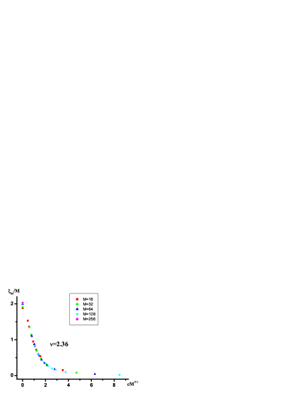
Figure 22: (Color online) Numerical results for fully chiral triangular network model. A fit of data to a one-parameter scaling form, $\xi_{M}/M=f(\varepsilon M^{1/\nu})$ yields the critical exponent, $\nu\approx 2.36$.

In Ref. Triangular, the critical exponent of the triangular model Fig. 20 was inferred from the real space renormalization group analysis. The result, $\nu\approx 2.3\div 2.76$, agrees with simulations of the CC model reported in the literature. Here we present the result of numerical simulations of the triangular model. Simulations use the slice transfer matrix

$$\mathbf{T}=\prod_{n=N-1}^{0}\mathbf{L}_{2}\mathbf{P}_{2}^{(n)}\mathbf{L}_{1}\mathbf{P}_{1}^{(n)},$$ (85)

Operators $\mathbf{L}_{1}$ and $\mathbf{L}_{2}$ act in ”white” and ”blue” stripes in Fig. 20, respectively. The operator $\mathbf{L}_{1}$ performs transformation of the vector of amplitudes, $\{Z_{i}^{(n)}\}$, into $\{\tilde{Z}_{i}^{(n+1)}\}$, while $\mathbf{L}_{2}$ performs transformation of $\{\tilde{Z}_{i}^{(n)}\}$ into $\{Z_{i}^{(n)}\}$, see Fig. 20. For a particular stripe width, $M=8$, the matrix forms of $\mathbf{L}_{1}$ and $\mathbf{L}_{2}$ are the following

$$\mathbf{L}_{1}=\left(\begin{array}[]{cccc|cccc}x_{11}&x_{12}&x_{13}&0&\cdot&\cdot&\cdot&\cdot\\ x_{21}&x_{22}&x_{23}&0&\cdot&\cdot&\cdot&\cdot\\ x_{31}&x_{32}&x_{33}&0&\cdot&\cdot&\cdot&\cdot\\ 0&0&0&1&\cdot&\cdot&\cdot&\cdot\\ \hline\cr\cdot&\cdot&\cdot&\cdot&x_{11}&x_{12}&x_{13}&0\\ \cdot&\cdot&\cdot&\cdot&x_{21}&x_{22}&x_{23}&0\\ \cdot&\cdot&\cdot&\cdot&x_{31}&x_{32}&x_{33}&0\\ \cdot&\cdot&\cdot&\cdot&0&0&0&1\end{array}\right),$$ (94)

$$\mathbf{L}_{2}=\left(\begin{array}[]{cc|cccc|cc}x_{33}&0&\cdot&\cdot&\cdot&\cdot&x_{31}&x_{32}\\ 0&1&\cdot&\cdot&\cdot&\cdot&0&0\\ \hline\cr\cdot&\cdot&x_{11}&x_{12}&x_{13}&0&\cdot&\cdot\\ \cdot&\cdot&x_{21}&x_{22}&x_{23}&0&\cdot&\cdot\\ \cdot&\cdot&x_{31}&x_{32}&x_{33}&0&\cdot&\cdot\\ \cdot&\cdot&0&0&0&1&\cdot&\cdot\\ \hline\cr x_{13}&0&\cdot&\cdot&\cdot&\cdot&x_{11}&x_{12}\\ x_{23}&0&\cdot&\cdot&\cdot&\cdot&x_{21}&x_{22}\end{array}\right),$$ (103)

with dots standing for zeroes. In the above relations, $\{x_{ij}\}$ form a $3\times 3$ matrix, $\mathbf{X}$, which is the node transfer matrix corresponding to the scattering matrix Eq. (84), and up to $\varepsilon^{2}$ terms has the matrix form

$$\mathbf{X}=\left(\begin{array}[]{ccc}2(1+\varepsilon)&-2(1+\varepsilon)&1\\ \\ 2(1+\varepsilon)&-3&2(1-\varepsilon)\\ \\ 1&-2(1-\varepsilon)&2(1-\varepsilon)\end{array}\right).$$ (109)

Specific form of $\mathbf{L}_{2}$ accounts for the cyclic boundary conditions in the vertical direction. Matrices

$$\mathbf{P}_{1}^{(n)}=\text{diag}\{e^{i\varphi_{1}^{(n)}},\cdots,e^{i\varphi_{8}^{(n)}}\}$$ (110)

and

$$\mathbf{P}_{2}^{(n)}=\text{diag}\{e^{i\psi_{1}^{(n)}},\cdots,e^{i\psi_{8}^{(n)}}\}.$$ (111)

account for the random phases on the links.

Similarly to CC model, the critical properties of the triangular model were inferred from the scaling analysis of the Lyapunov exponents. The scaling plot is shown in Fig. 22. A high quality scaling was achieved for $\nu=2.36$, which is in a good agreement with simulations of the CC model.

VI.2 Numerical results for the triangular p-q model

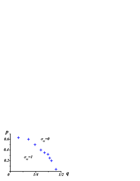
Figure 23: (Color online) Numerical results for the line of delocalization transitions in triangular p-q model. The point $q=0$ corresponds to $p=p_{c}=0.6527$- threshold of bond percolation on hexagonal lattice.

In the CC model, which is based on the picture of equipotentials, the scattering matrix at a node, $S_{CC}$, is a function of energy, $\varepsilon$. By contrast, in the p-q model, describing low magnetic fields, the scattering matrix at the node depends on ”magnetic field”, $1/2-q$, while the energy dependence enters via the backscattering probability, $p$. Still, the structure of the scattering matrices of the CC model and the p-q model are the same. It is also the case for the triangular p-q model, for which we choose the following form of the $q$- dependent scattering matrix

$$S=\frac{1}{q^{2}-q+1}\left(\begin{array}[]{ccc}1-q&q(q-1)&q\\ \\ q&1-q&q(q-1)\\ \\ q(q-1)&q&1-q\end{array}\right).$$ (112)

This matrix is unitary for all $0\leq q\leq 1$. It is critical at $q=1/2$. Indeed, as follows from Eq. (112), the ratio of probabilities of scattering to the left and to the right is $q/(1-q)$, so that at $q=1/2$ these probabilities are equal. Their values are $4/9$ in agreement with Eq. (84). With this parametrization, the $6\times 6$ junction scattering matrix in Fig. 19 acquires the form

$${\scriptstyle\frac{1}{q^{2}-q+1}}\!\left(\!\begin{array}[]{cccccc}{\scriptstyle 0}&\!\!{\scriptstyle 1-q}&\!\!{\scriptstyle 0}&\!\!{\scriptstyle q(q-1)}&\!\!{\scriptstyle 0}&\!\!{\scriptstyle q}\\ {\scriptstyle 1-q}&\!\!{\scriptstyle 0}&\!\!{\scriptstyle q(q-1)}&\!\!{\scriptstyle 0}&\!\!{\scriptstyle q}&\!\!{\scriptstyle 0}\\ {\scriptstyle 0}&\!\!{\scriptstyle q}&\!\!{\scriptstyle 0}&\!\!{\scriptstyle 1-q}&\!\!{\scriptstyle 0}&\!\!{\scriptstyle q(q-1)}\\ {\scriptstyle q}&\!\!{\scriptstyle 0}&\!\!{\scriptstyle 1-q}&\!\!{\scriptstyle 0}&\!\!{\scriptstyle q(q-1)}&\!\!{\scriptstyle 0}\\ {\scriptstyle 0}&\!\!{\scriptstyle q(q-1)}&\!\!{\scriptstyle 0}&\!\!{\scriptstyle q}&\!\!{\scriptstyle 0}&\!\!{\scriptstyle 1-q}\\ {\scriptstyle q(q-1)}&\!\!{\scriptstyle 0}&\!\!{\scriptstyle q}&\!\!{\scriptstyle 0}&\!\!{\scriptstyle 1-q}&\!\!{\scriptstyle 0}\end{array}\!\!\!\right).$$ (113)

Since backscattering in triangular p-q model, Fig. 20, takes place on the links, it is described by the same $2\times 2$ matrix Eq. (32) as in the square p-q model. Thus, by analogy to Eq. (73), the $T$- matrix of the triangular p-q model has the form

$$\hat{\text{\large T}}=\!\left(\!\!\begin{array}[]{cccccc}\tilde{x}_{11}&0&0&\tilde{x}_{12}&\tilde{x}_{13}&0\\ 0&x_{11}&x_{12}&0&0&x_{13}\\ 0&x_{21}&x_{22}&0&0&x_{23}\\ \tilde{x}_{21}&0&0&\tilde{x}_{22}&\tilde{x}_{23}&0\\ \tilde{x}_{31}&0&0&\tilde{x}_{32}&\tilde{x}_{33}&0\\ 0&x_{31}&x_{32}&0&0&x_{33}\end{array}\right)\hat{\text{\large D}}_{1}\left(\!\!\begin{array}[]{cccccc}{\scriptstyle\frac{1}{\sqrt{1-p}}}&{\scriptstyle\sqrt{\frac{p}{1-p}}}&0&0&0&0\\ {\scriptstyle\sqrt{\frac{p}{1-p}}}&{\scriptstyle\frac{1}{\sqrt{1-p}}}&0&0&0&0\\ 0&0&{\scriptstyle\frac{1}{\sqrt{1-p}}}&{\scriptstyle\sqrt{\frac{p}{1-p}}}&0&0\\ 0&0&{\scriptstyle\sqrt{\frac{p}{1-p}}}&{\scriptstyle\frac{1}{\sqrt{1-p}}}&0&0\\ 0&0&0&0&{\scriptstyle\frac{1}{\sqrt{1-p}}}&{\scriptstyle\sqrt{\frac{p}{1-p}}}\\ 0&0&0&0&{\scriptstyle\sqrt{\frac{p}{1-p}}}&{\scriptstyle\frac{1}{\sqrt{1-p}}}\end{array}\!\!\right)\hat{\text{\large D}}_{2},$$ (114)

where the diagonal matrices

$$\hat{\text{\large D}}_{1}=\text{diag}\{e^{i\varphi_{1}},\cdots,e^{i\varphi_{6}}\}$$ (115)

and

$$\hat{\text{\large D}}_{2}=\text{diag}\{e^{i\psi_{1}},\cdots,e^{i\psi_{6}}\}$$ (116)

account for the random phases on the links. The matrix, $\{x_{ij}\}=\text{\large X}$, has the explicit $q$- dependence

$$\text{\large X}(q)=\left(\begin{array}[]{ccc}\frac{1}{q}&-\frac{1}{q}&1\\ \\ \frac{1}{q}&\frac{q^{2}-q+1}{q(q-1)}&\frac{1}{q-1}\\ \\ 1&\frac{1}{1-q}&\frac{1}{1-q}\end{array}\right),$$ (117)

and $\{\tilde{x}_{ij}\}=\tilde{\text{\large X}}$ are given by the relation

$$\tilde{\text{\large X}}(q)=\text{\large X}^{-1}(1-q).$$ (118)

In the square p-q model, two prominent points on the $p,q$ plane were $(\frac{1}{2},0)$ and $(0,\frac{1}{2})$. They corresponded to the bond percolation over p- and q- bonds, respectively. Similarly, in the triangular p-q model, the point $(0,\frac{1}{2})$ is distinguished. At this point, due to the absence of p- bonds, two decoupled q- subnetworks undergo the site percolation. In triangular p-q model, the counterpart of the p- bond percolation at $(\frac{1}{2},0)$ of the square p-q model is a p- bond percolation on a hexagonal lattice. This is because the centers of forbidden regions in Fig. 19 constitute a hexagonal lattice. Thus, the second distinguished point for triangular p-q model should be $(p_{c},0)$, where

$$p_{c}=1-2\sin\left(\frac{\pi}{18}\right)=0.6527$$ (119)

is the threshold of the bond percolation on the honeycomb lattice SykesEssam . Our numerical simulations based on the transfer matrix Eq. (114) confirm this expectation. The points of the delocalization transition, shown in Fig. 23 follow the line which smoothly connects the point $(0.6527,0)$ and $(0,\frac{1}{2})$. The general shape of the line is quite similar to the above results, Fig. 8, for the square p-q model. In particular, in the domain of vanishing magnetic fields, $(1/2-q)\ll 1$, the transition boundary is again linear, in agreement with prediction Eq. (8) of the scaling theory.

In conclusion of this section we would like to make the following remark. Simplification of the node structure in the square p-q model was achieved by choosing the matrix Eq. (48) which captures orbital action of magnetic field, but does not allow forward- and backward scattering, which, instead, takes place on the links. Similarly, in the triangular p-q model, the junction matrix Eq. (113) restricts the scattering options for incident electrons. Namely, out of six possibilities, the electron can be scattered only into three channels. Again, similarly to the square p-q model, it can access the three other channels upon backscattering on the links.

VII Strongly localized region: implications for inelastic transport

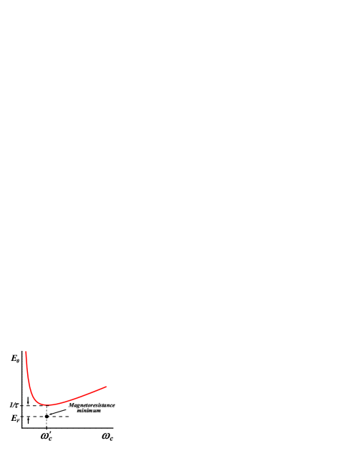
Figure 24: (Color online) Levitation plot for $n=0$; same as lower curve in Fig. 1. For electron densities corresponding to $E_{F}$ slightly below the minimum, inelastic magnetoresistance has a deep minimum near magnetic field, $\omega_{c}=\omega_{c}^{\prime}$.

The presence of a minimum in the line, $E_{n}(\omega_{c})$, of the delocalization transitions, Fig. 1, manifests itself in specific behavior of low-temperature magnetoresistance, $\rho_{xx}(\omega_{c})$. For high enough electron densities, $\rho_{xx}(\omega_{c})$ is temperature independent at two (low and high) distinct values of magnetic field. This $T$- independence is a signature of the delocalization transition. Different experimental groups have studied details of the behavior of $\rho_{xx}(\omega_{c},T)$ near the high-field transition shahar95 ; shahar96 ; dunford00 ; Ponomarenko07 , low-field transition shahar97 ; shahar'97 , or both transitions Exp6 ; hilke97 ; hilke98 ; hilke00 ; murzin02 ; yasin02 . For Fermi level position below the minimum in Fig. 1, the system remains localized upon increasing $\omega_{c}$, see Fig. 24. However, even in this localized regime, proximity of $\omega_{c}$ to the position of minimum, $\omega_{c}^{\prime}$, (Fig. 24) should manifest itself as a precursor of delocalization in the inelastic transport. Such a precursor of delocalization has actually been observed in the early papers Jiang92 ; Koch92 in the form of a minimum in $\rho_{xx}(\omega_{c})$, in the regime of the variable-range hopping. This minimum reflects the increase of localization radius, $\xi(\omega_{c})$, near $\omega_{c}=\omega_{c}^{\prime}$. The lower is the temperature, the deeper is minimum, as follows from the Mott’s law

$$\ln\left[\rho_{xx}(\omega_{c})\right]\propto\frac{1}{\left[\xi^{2}(\omega_{c})T\right]^{1/3}}.$$ (120)

Theoretical studies of variable-range-hopping magnetoresistance pertained to deeply localized regime, where interference effects in a single hopping act constituted a small but singular in $\omega_{c}$ correction to the tunneling probability Shklovskii85 ; Shklovskii86 . The correction is small because the tunneling probability is greatly reduced if electron under-barrier trajectory deviates from the straight line. According to Refs. Shklovskii85, , Shklovskii86, , interference responsible for magnetoresistance occurs between different virtual forward-tunneling trajectories. The other early theory Ref. AAK82, of negative hopping magnetoresistance was based on the following reasoning. Weak magnetic field, by changing the universality class and thus inducing delocalization of states with high energies, $\gtrsim 1/\tau$, causes some growth of $\xi$ for the states in the deep tail. Note that both theories, as well as later theory Ref. Glazman, , were based on the phase rather than orbital action of magnetic field.

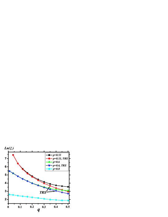
Figure 25: (Color online) Localization radius in the strongly localized region $p>1/2$ is plotted vs. magnetic field. The point $q=0$ represents the field, $\omega_{c}=\omega^{\prime}_{c}$ in Fig. 24. Red and black curves for $p=0.53$, and blue and green curves for $p=0.6$ corresponding to TRS and no TRS, respectively, merge upon increasing magnetic field. Light blue curve corresponds to $p=0.8$. There is no difference between TRS and no TRS for this deeply localized energy.

By now there is no theory describing the behavior of localization radius, $\xi(E_{\scriptscriptstyle F},\omega_{c})$, in the domain of intermediate fields $\omega_{c}\sim\omega_{c}^{\prime}\sim 1/\tau$ and electron densities ( Fermi energies, $E_{\scriptscriptstyle F}$) at which electron states are localized but not strongly, so that $E_{\scriptscriptstyle F}\tau\sim k_{\scriptscriptstyle F}l\sim 1$. On the other hand, the p-q model offers a unique possibility to study localization length in this domain. To this end, we studied numerically $\xi(p,q)$ in the region $p>1/2$ on the $p,q$ plane. The dependence $\xi(p,q)$ can be translated into the $\xi(E_{\scriptscriptstyle F},\omega_{c})$ dependence. We find that the phase action of magnetic field does lead to a certain increase in $\xi$ at low fields. However, further increase of $\omega_{c}$, when the orbital action sets in, causes a much stronger delocalization effect.

Our numerical results for $\xi(p,q)$ are presented in Fig. 25, for the values $p=0.53,\,0.6,$ and $0.8$. In order to illuminate the role of the mechanism Refs. Shklovskii85, , Shklovskii86, , simulations were performed with and without TRS on the links. The values of $\xi(p,q)$ were inferred from the scaling analysis of $\xi_{M}/M$, similarly to the case of zero magnetic field. For $p=0.8$, the difference between TRS and no-TRS is negligibly small. Still the interplay of orbital effect and interference leads to enhancement of $\xi$ from weak, $q=1/2$, to strong, $q=0$, magnetic fields, by a factor of $2$. From Eq. (120) it follows that the corresponding drop-off of log-resistance is $2^{2/3}$, and $\ln(\rho)$ is approximately linear in $(1/2-q)$. This allows a comparison with the experimental data of Ref. Jiang92, , where giant negative hopping magnetoresistance of a degenerate 2D electron gas was reported. For experimental value of $\xi=250\,\AA$ the low-field log-resistance at temperature, $T=0.3K$, was $8.7$. The net drop-off of log-resistance observed was $2.3$. This corresponds to the increase of $\xi$ by a factor of $1.5$. However, at $p=0.8$ our numerics suggests a linear change of $\xi$ with $q$, while experimentally it changes slower. The possible origin of this discrepancy lies in the fact that $(1/2-q)$ is proportional to $\omega_{c}$ only at low fields. In fact, at higher fields, $(1/2-q)$ changes slower than $\omega_{c}$.

As $p$ decreases towards $1/2$, both phase and orbital mechanisms of magnetoresistance become stronger. As follows from Fig. 25, the (zero-field) $\xi$ increases from TRS to no TRS by a factor $1.47$ and $1.82$ for $p=0.6$ and $p=0.53$, respectively. This increase is a quantitative measure of the phase mechanism. It should result in drop-off of the log-resistance by the factors $1.3$ and $1.5$, which corresponds to the resistance drop by several times. The orbital mechanism causes a significantly bigger reduction of log-resistance. The $p=0.6$ and $p=0.53$ curves in Fig. 25 indicate the decrease in $\xi$ between $q=0$ and $q=0.5$ by factors $11$ and $60$, respectively. Both effects are way too strong in comparison with all the experimental data on hopping transport reported in the literature. This is because $p=0.6$ and $p=0.53$ correspond to very large values of localization radius, e.g., $\xi=3000\AA$ in experimental conditions of Ref. Jiang92, . Temperatures required to observe hopping transport with such large $\xi$ are unreasonably low.

VIII Conclusion

It is expected on general grounds that, as disordered system undergoes a quantum Hall transition, its behavior is universal, i.e., in the vicinity of transition this behavior does not depend on the type of disorder. For quantum Hall transition in a strong magnetic field numerics provides a compelling evidence for such a universality. For example, critical exponent derived from the CC model, based on the picture of a smooth disorder, and from the simulations Huckestein90 for the point-like scatterers are the same.

Scaling scenario of Ref. AALR, suggests that regardless of the type of the disorder, a single characteristics of the system, the Drude conductance $\sigma$, determines the size of the sample, $\xi_{o}$ or $\xi_{u}$, depending on presence or absence of TRS, at which the system becomes an insulator. By virtue of scaling scenario, electron moving on the links of the network and scattered at the nodes gets localized, due to interference effects, in the same way as realistic electron moving on a plane and scattered by random impurities. Correspondence between two systems is established by Eq. (16).

Pruisken’s theory suggests that, in magnetic field, only two characteristics, the components $\sigma_{xx}$ and $\sigma_{xy}$ of the Drude conductivity tensor determine what value of quantized Hall conductivity the system will acquire at large scales, when the interference effects suppress the diagonal conductivity.

Basing on insensitivity to the character of disorder, we expect that weakly chiral network of junctions and point contacts represents electron gas in a non-quantizing magnetic field. To establish the correspondence we need to express the values of $\sigma_{xx}$ and $\sigma_{xy}$ of our network in terms of parameters $p$ and $q$ in the Drude regime, i.e., the regime where the interference can be neglected. Above we have already identified $(k_{\scriptscriptstyle F}l)^{-1}$ with parameter $p$ of the p-q model. Here we elaborate on this relation.

Our main idea of modelling a competition between interference-induced localization and magnetic-field-induced orbital curving is to confine the orbital action to a set of compact spatial regions-junctions, with asymmetry of scattering to the left and to the right proportional to magnetic field. In zero field, these junctions represent strong scatterers of electrons. These strong scatterers come in addition to weak ”intrinsic” scatterers, that limit the mean free path, $l$, of electron gas. If strong scatterers are sparse, they will not affect the transport of electron gas at all. On the other hand, if they are dense, then the mobility will be limited exclusively by scattering off these strong scatterers. This suggests that the distance between the scatterers should be chosen of the order of $l$. Therefore, as we replace realistic electron motion by a motion along the links of a network, the dimensionless lattice constant should be chosen as $\sim k_{\scriptscriptstyle F}l$.

In our p-q network Fig. 5, in addition to junctions (strong scatterers) there are point contacts on the links. The role that these point contacts play is the following. Our junctions Fig. 5 do not provide any backscattering. More precisely, as can be seen from Fig. 5, an electron starting along a given link, say, to the right, after several scatterings off the junctions, will never return to the starting point from the left. Thus, the junctions alone cannot model the interference effects in realistic electron gas, where the probability of such a return is $\sim 1/(k_{\scriptscriptstyle F}l)$. It is the point contacts that provide possibility of backscattering in the p-q network, and parameter $p$ is chosen $1/(k_{\scriptscriptstyle F}l)$ in order to model the realistic return probability.

From the above reasoning, the diagonal conductivity of the p-q model is $\sigma_{xx}\sim 1/p$. In a finite magnetic field, estimate for $\sigma_{xy}$ can be found from Eq. (49):

$$\sigma_{xy}=R_{H}\sigma_{xx}\sim\left(\frac{1}{2}-q\right)\sigma_{xx}\sim\frac{1/2-q}{p}.$$ (121)

Note now, that the boundary of delocalization transition established in the present paper, is $\alpha(1/2-q)=p$ with $\alpha\sim 1$. Then we conclude from Eq. (121) that transition occurs when the ”Boltzmann” value of $\sigma_{xy}$ is $\sim 1$. On the other hand, levitation scenario is based on the conjecture that the classical $\sigma_{xy}=1$ does not get renormalized upon increasing the sample size, see Eqs. (5), (6). Consistency between delocalization condition within p-q model and within scaling theory Khmelnitskii can be viewed as evidence that the p-q model adequately captures microscopic physics behind the levitation scenario.

There is a fundamental reason why the picture of the weak-field quantum Hall transition is much more complex than the picture of the strong-field transition. Namely, for strong-field transition there is an exact duality of electron states above and below critical energy. By contrast, there is no such inherent duality in the weak-field transition. This, in particular, does not allow to employ the quantum real-space renormalization group approach Triangular ; aram ; arovas ; cain ; cain03 ; reviews to describe this transition analytically.

Duality with respect to the center, $\varepsilon=0$, of the Landau level in the CC model insures that, with a strong spread in the saddle-point heights, the scaling region narrows, but delocalized state remains at $\varepsilon=0$. A remarkable outcome of our numerics is that the same property holds for the weak-field transition: we have verified that, upon introducing a strong spread in the local values of the backscattering strength, $p$, but keeping $\langle p\rangle$ fixed, does not effect the position, $p_{c}(q)$, of the transition point. On the other hand, upon increasing the spread in the local values of $p$, interference effects become progressively less relevant. This allowed us to uncover a transparent classical picture of the low-field quantum Hall transition, see Figs. 9, 10, which is a counterpart of the percolation picture of the strong-field transition Kazarinov ; Iordansky ; Trugman . The fact that levitation emerges both within the p-q model and from the scaling equations Eqs. (5), (6), still does not mean that the p-q model offers a microscopic support for the Pruisken theory. After all, phenomenon of levitation follows from a general argument that delocalized states have nowhere to go but up in the vanishing magnetic field. In fact, scaling equations Eqs. (5), (6) suggest a stronger message: namely, positions of delocalized states do not change if magnetic field does not exercise any ”phase” action. Neglecting the phase action corresponds to replacement of the first term in Eq. (5) by a constant. We emphasize that the p-q model supports this prediction of the Pruisken theory. This is reflected in the coincidence (within accuracy of our numerics) of the p-q boundary with and without TRS.

In closing, we list the questions which were previously addressed in the frame of fully chiral CC model and are also pertinent to the weakly chiral p-q model:

(i). Two-channel network models of CC type were studied in Refs. Kagalovsky95, ; kagalovsky97, ; LeeChalker94, ; LeeChalkerKo94, ; wen94, ; kagalovsky99, ; gruzberg99, in connection with spin-orbit induced splitting of quantum Hall transition LeeChalker94 ; LeeChalkerKo94 , disorder-induced ”attraction” of delocalized states from different Landau levels wen94 ; Kagalovsky95 ; kagalovsky97 and quantum Hall transition in disordered superconductors kagalovsky99 ; gruzberg99 . All these considerations are based on two co-propagating channels on each link. In p-q model, the two channels are counter-propagating and spinless. It would be interesting to incorporate spin-orbit coupling into the p-q model for the following reason. In zero magnetic field and in the presence of spin-orbit coupling there is a critical energy above which electron states are delocalized SO ; Asada04 . On the other hand, in strong magnetic fields, spin-orbit coupling splits discrete delocalized states LeeChalker94 ; LeeChalkerKo94 . Upon decreasing the magnetic field, both delocalized states are most likely to head towards zero-field metal-insulator transition point. Microscopic model describing this scenario must include orbital action of magnetic field, spin-orbit coupling, and interference effects. This can be accomplished upon incorporating spin degree of freedom into the p-q model. A possible application of the above physics is graphene in a weak magnetic filed Furusaki . In the latter case, the inter-valley scattering plays the role of spin-orbit coupling.

(ii). In three dimensional layered system in zero magnetic field, arbitrarily weak coupling between the layers delocalizes electron states above a certain critical energy. In strong magnetic field, a weak interlayer coupling smear discrete delocalized state into metallic band Dohmen . Matching of these two scenarios takes place in weak magnetic fields. The p-q model based description can be employed in this domain.

(iii). Interaction-induced dephasing wang00 is crucial for experimental observability of levitation, since the transition is smeared when localization radius exceeds the dephasing length. The issue closely related to dephasing is a peculiar behavior of the non-diagonal resistivity, $\rho_{xy}$, in the vicinity of the high-field transition dykhne94 ; ruzin95 ; shimshoni97 ; pryadko ; pryadko00 ; Zulicke ; Shimshoni04 ; apalkov03 . The question about behavior of $\rho_{xy}$ near the low-field transition point can be asked and addressed within ”incoherent” p-q model. In addition, the question about interplay of disorder and interaction previously studied for high-field transition cobden99 ; mahida01 ; Faulhaber05 ; yang95 ; huckestein99 ; yang01 ; wang02 , can be redirected to the low-field transition.

(iv). It is known that there is an intimate relation between delocalization transition in CC model and critical behavior of superspin chains DHLee94 ; Zirnbauer94 ; Zirnbauer97 ; Kim96 ; Gruzberg97 ; Marston99 . It would be interesting to investigate wether the p-q model corresponds to any spin model. It is also known that CC model is related to the Dirac Hamiltonian with disorder Fisher94 ; HoChalker . Recall that at degeneracy point, $p=0$, $q=1/2$, the p-q model falls into two independent CC models. Modification of the mixing of two counter-propagating channels on the links transforms the p-q model with $q=1/2$ to the model studied in Ref. Bocquet, . This modification leads to criticality which was studied within the sigma-model approach Gade1 ; Gade2 . It would be interesting to investigate such a modification of the p-q model away from the degeneracy point. More specifically, the case $q\neq 1/2$, in our p-q model, differs from the model Ref. Bocquet, primarily in the scattering matrix of junctions. Our junction matrix Eq. (48) describes scattering, say, to the right, with the same probability $q$ for all incoming channels, while the nodes in Ref. Bocquet, describe scattering to the right with the probability $q$ from two opposite channels, and with the probability $(1-q)$ from the other two opposite channels. In terms of coupling of counter-propagating channels on the links, in Ref. Bocquet, this coupling differs from our link matrix in following respects: to get the coupling of Ref. Bocquet, one should replace in Eq. (73) the phases $\phi_{i}$ should all be put zero, while $\varphi_{i}$ satisfy the relation $\varphi_{1}=\varphi_{2}$, $\varphi_{3}=\varphi_{4}$, which is different even from the case with TRS in the p-q model.

IX Acknowledgements

We acknowledge fruitful discussions with I. Gruzberg. This work was supported by the BSF grant No. 2006201. One of us (V. K.) appreciates the hospitality of the MPI-PKS in Dresden, where significant part of his work was done.

X Appendix

The easiest way to derive Eq. (16) is to notice that with respect to the motion along the diagonal direction of network the diffusion has, effectively, a one-dimensional character Janssen . This is because the motion along the diagonal can be viewed as a random sequence of transmissions and reflections without deflections. For a given site, the full probability of transmission along the diagonal direction (say, up and to the right) is $\mathcal{T}=t^{2}+d^{2}$, while the full probability of reflection is $1-\mathcal{T}=r^{2}+d^{2}$. Parameter $k_{\scriptscriptstyle F}l$ should be identified with ratio, $\mathcal{T}/(1-\mathcal{T})$. Together with flux-conservation condition, $t^{2}+r^{2}+2d^{2}=1$, this ratio reduces to Eq. (16).

As we pointed out in Section II, the point $d=1/\sqrt{2}$ is singular: strong localization predicted by scaling theory with Boltzmann result Eq. (16) as an initial condition, contradicts to the result of Ref. Bocquet, . This contradiction can be resolved from the following reasoning.

The same average $\langle d^{2}\rangle$ can be realized in two completely different ways:

(i) Boltzmann approach. In the two instances of scattering at the same node, electron can be deflected both to the left and to the right with equal probabilities, $50\%$.

(ii) Percolative approach. A given node scatters always to the left or always to the right; $50\%$ of the nodes scatter to the left, and remaining $50\%$ scatter to the right.

Note, that the classical motion of electron is very different in the above two realizations. In the case (i) this motion is diffusive. Then interference will readily localize this motion. The case (ii) corresponds to classical percolation threshold. To see this, notice, that the electron predominantly travels in loops (clusters) and one trajectory is the infinite cluster spanning the entire system. In fact, it can be easily seen that possible trajectories belong to two decoupled bond-percolation networks. Interference will transform these networks to two CC models at the delocalization-transition points. Since the percolative picture is fully coherent, it captures properly the quantum delocalization, while ”dephased” Boltzmann picture does not.

Thus the distinguished characteristics of the point $d=1/\sqrt{2}$ is that only at this point there is sensitivity to the realization of the disorder.

Note that in the case $t=r=0$ but $d_{1}=\sqrt{1-d_{2}^{2}}$ not equal to $1/\sqrt{2}$, prediction of the scaling theory that the Boltzmann result governs localization properties at large distances is correct. Although with a strong spread in local $d$-values, when the network still breaks into two CC networks, the states of both CC networks are localized with localization radius, $\xi\sim|d_{1}^{2}-1/2|^{-4/3}$.

References

- (1) E. Abrahams, P. W. Anderson, D. C. Licciardello, and T. V. Ramakrishnan, Phys. Rev. Lett. 42, 673 (1979).
- (2) D. E. Khmelnitskii, Phys. Lett. 106A, 182 (1984); his prediction of levitation was based on analysis of RG flows, which he introduced earlier in JETP Lett. 38, 552 (1983).
- (3) A. M. M. Pruisken, Nucl. Phys. B235, [FS11], 277 (1984); A.M.M. Pruisken and I.S. Burmistrov, Ann. Phys. 316, 285 (2005).
- (4) R. Laughlin, Phys. Rev. Lett. 52, 2304 (1984).
- (5) S. Kivelson, D.-H. Lee, and S.-C. Zhang, Phys. Rev. B 46, 2223 (1992).
- (6) H. W. Jiang, C. E. Johnson, and K. L. Wang, Phys. Rev. B 46, 12830 (1992).
- (7) C. E. Johnson and H. W. Jiang, Phys. Rev. B 48, 2823 (1993).
- (8) H. W. Jiang, C. E. Johnson, K. L. Wang, and S. T. Hannahs, Phys. Rev. Lett. 71, 1439 (1993).
- (9) I. Glozman, C. E. Johnson, and H. W. Jiang, Phys. Rev. Lett. 74, 594 (1995).
- (10) I. Glozman, C. E. Johnson, and H. W. Jiang, Phys. Rev. B 52, R14348 (1995).
- (11) S. C. Dultz, H. W. Jiang, and W. J. Schaff, Phys. Rev. B 58, R7532 (1998).
- (12) S. Kravchenko, W. Mason, J. Furneaux, and V. Pudalov, Phys. Rev. Lett. 75, 910 (1995).
- (13) T. Wang, K. P. Clark, G. F. Spencer, A. M. Mack, and W. P. Kirk, Phys. Rev. Lett. 72, 709 (1994).
- (14) J. F. Hughes, J. T. Nicholls, J. E. F. Frost, E. H. Linfield, M. Pepper, C. J. B. Ford, D. A. Ritchie, G. A. C. Jones, E. Kogan, and M. Kaveh, J. Phys.: Condens. Matter 6, 4763 (1994).
- (15) S.-H. Song, D. Shahar, D. C. Tsui, Y. H. Xie, and D. Monroe, Phys. Rev. Lett. 78, 2200 (1997).
- (16) G. Xiong, S.-D. Wang, Q. Niu, De-C. Tian, and X. R. Wang, Phys. Rev. Lett. 87, 216802 (2001).
- (17) D. Z. Liu, X. C. Xie, and Q. Niu, Phys. Rev. Lett. 76, 975 (1996).
- (18) K. Yang and R. N. Bhatt, Phys. Rev. Lett. 76, 1316 (1996).
- (19) D. N. Sheng and Z. Y. Weng, Phys. Rev. Lett. 78, 318 (1997).
- (20) D. N. Sheng and Z. Y. Weng, Phys. Rev. Lett. 80, 580 (1998).
- (21) D. N. Sheng and Z. Y. Weng, Phys. Rev. B 62, 15363 (2000).
- (22) Th. Koschny, H. Potempa, and L. Schweitzer, Phys. Rev. Lett. 86, 3863 (2001).
- (23) D. N. Sheng, Z. Y. Weng, and X. G. Wen, Phys. Rev. B 64, 165317 (2001).
- (24) X. Wan and R. N. Bhatt, Phys. Rev. B 64, 201313 (2001).
- (25) Th. Koschny and L. Schweitzer, Phys. Rev. B 70, 165301 (2004).
- (26) B. Huckestein, Phys. Rev. Lett. 84, 3141 (2000).
- (27) T. V. Shahbazyan and M. E. Raikh, Phys. Rev. Lett. 75, 304 (1995).
- (28) V. Kagalovsky, B. Horovitz, and Y. Avishai, Phys. Rev. B 52, R17044 (1995).
- (29) V. Kagalovsky, B. Horovitz, and Y. Avishai, Phys. Rev. B 55, 7761 (1997).
- (30) A. Gramada and M. E. Raikh, Phys. Rev. B 54, 1928 (1996).
- (31) F. D. M. Haldane and K. Yang, Phys. Rev. Lett. 78, 298 (1997).
- (32) M. M. Fogler, Phys. Rev. B 57, 11947 (1998).
- (33) A. L. C. Pereira and P. A. Schulz, Phys. Rev. B 66, 155323 (2002).
- (34) A. MacKinnon and B. Kramer, Phys. Rev. Lett. 47, 1546 (1981).
- (35) P. W. Anderson, Phys. Rev. 109, 1492 (1958).
- (36) B. Shapiro, Phys. Rev. Lett. 48, 823 (1982).
- (37) R. Merkt, M. Janssen, and B. Huckestein Phys. Rev. B 58, 4394 (1998).
- (38) S. Hikami, A. I. Larkin, and Y. Nagaoka, Prog. Theor. Phys. 63, 707 (1980).
- (39) J. T. Chalker and P. D. Coddington, J. Phys. C 21, 2665 (1988).
- (40) R. F. Kazarinov and S. Luryi, Phys. Rev. B 43, 7626 (1982).
- (41) S. V. Iordansky, Solid State Commun. 43, 1 (1982).
- (42) S. A. Trugman, Phys. Rev. B 27, 7539 (1983).
- (43) H. P. Wei, S. W. Hwang, D. C. Tsui, and A. M. M. Pruisken, Surf. Sci. 229, 34 (1990).
- (44) W. Pan, D. Shahar, D. C. Tsui, H. P. Wei, and M. Razeghi, Phys. Rev. B 55, 15431 (1997).
- (45) R. T. F. van Schaijk, A. de Visser, S. M. Olsthoorn, H. P. Wei, and A. M. M. Pruisken, Phys. Rev. Lett. 84, 1567 (2000).
- (46) S. Koch, R. J. Haug, K. v. Klitzing, and K. Ploog, Phys. Rev. Lett. 67, 883 (1991).
- (47) W. Li, G. A. Csathy, D. C. Tsui, L. N. Pfeiffer, and K. W. West, Phys. Rev. Lett. 94, 206807 (2005).
- (48) W. Li, C. L. Vicente, J. S. Xia, W. Pan, D. C. Tsui, L. N. Pfeiffer, and K. W. West, Phys. Rev. Lett. 102, 216801 (2009).
- (49) D. H. Cobden and E. Kogan Phys. Rev. B 54, R17316 (1996).
- (50) F. Hohls, U. Zeitler, R. J. Haug, Phys. Rev. B 66, 073304 (2002).
- (51) E. Peled, D. Shahar, Y. Chen, D. L. Sivco, and A. Y. Cho, Phys. Rev. Lett. 90, 246802 (2003).
- (52) K. Slevin and T. Ohtsuki, Phys. Rev. B 80, 041304 (2009).
- (53) R. Klesse and M. Metzler, Phys. Rev. Lett. 79, 721 (1997).
- (54) Z. Wang, B. Jovanović, and D.-H. Lee, Phys. Rev. Lett. 77, 4426 (1996).
- (55) S. Cho and M. P. A. Fisher, Phys. Rev. B 55, 1637 (1997).
- (56) M. Janssen, M. Metzler, and M. R. Zirnbauer, Phys. Rev. B 59, 15836 (1999).
- (57) Extensive literature on the CC model can be found in the review B. Kramer, T. Ohtsuki, S. Kettemann, Phys. Rep. 417, 211 (2005).
- (58) V. V. Mkhitaryan, V. Kagalovsky, and M. E. Raikh, Phys. Rev. Lett. 103, 066801 (2009).
- (59) M. Bocquet and J. T. Chalker, Phys. Rev. B 67, 054204 (2003).
- (60) D. G. Ravenhall, H. W. Wyld, and R. L. Schult, Phys. Rev. Lett. 62, 1780 (1989).
- (61) H. U. Baranger and A. D. Stone, Phys. Rev. Lett. 63, 414 (1989).
- (62) C. W. Beenakker and H. van Houten, Phys. Rev. Lett. 63, 1857 (1989).
- (63) G. Timp, A. M. Chang, P. Mankiewich, R. Behringer, J. E. Cunningham, T. Y. Chang and R. E. Howard, Phys. Rev. Lett. 59, 732 (1987).
- (64) M. L. Roukes, A. Scherer, S. J. Allen, Jr., H. G. Craighead, R. M. Ruthen, E. D. Beebe and J. P. Harbison, Phys. Rev. Lett. 59, 3011 (1987).
- (65) A. M. Chang, G. Timp, T. Y. Chang, J. E. Cunningham, P. M. Mankiewich, R. E. Behringer and R. E. Howard, Solid State Commun. 67, 769 (1988).
- (66) C. J. B. Ford, T. J. Thornton, R. Newbury, M. Pepper, H. Ahmed, D. C. Peacock, D. A. Ritchie, J. E. F. Frost, and G. A. C. Jones, Phys. Rev. B 38, 8518 (1988).
- (67) J. A. Simmons, D. C. Tsui and G. Weimann, Surf. Sci. 196, 81 (1988).
- (68) D.-H. Lee, Z. Wang, and S. Kivelson, Phys. Rev. Lett. 70, 4130 (1993).
- (69) P. J. Reynolds, W. Klein, and H. E. Stanley, J. Phys. C 10, L167 (1977).
- (70) D. G. Polyakov and B. I. Shklovskii, Phys. Rev. B 48, 11167 (1993).
- (71) D. K. K. Lee and J. T. Chalker, Phys. Rev. Lett. 72, 1510 (1994).
- (72) D. K. K. Lee, J. T. Chalker, and D. Y. K. Ko, Phys. Rev. B 50, 5272 (1994).
- (73) C. B. Hanna, D. P. Arovas, K. Mullen, and S. M. Girvin, Phys. Rev. B 52, 5221 (1995).
- (74) A. Gramada and M. E. Raikh, Phys. Rev. B 56, 3965 (1997).
- (75) We are indebted to I. Gruzberg for this argument.
- (76) V. V. Mkhitaryan and M. E. Raikh, Phys. Rev. B 79, 125401 (2009).
- (77) M. F. Sykes and J. W. Essam, Phys. Rev. Lett. 10, 3 (1963).
- (78) D. Shahar, D. C. Tsui, M. Shayegan, R. N. Bhatt, and J. E. Cunningham, Phys. Rev. Lett. 74, 4511 (1995).
- (79) D. Shahar, D. C. Tsui, M. Shayegan, E. Shimshoni, and S. L. Sondhi, Science 274, 589 (1996).
- (80) R. B. Dunford, N. Griffin, M. Pepper, P. J. Phillips, and T. E. Whall, Physica E 6, 297 (2000).
- (81) D. T. de Lang, L. A. Ponomarenko, A. de Visser, and A. M. Pruisken, Phys. Rev. B 75, 035313 (2007).
- (82) D. Shahar, D. C. Tsui, M. Shayegan, E. Shimshoni, and S. L. Sondhi, Phys. Rev. Lett. 79, 479 (1997).
- (83) D. Shahar, M. Hilke, C. C. Li, D. C. Tsui, S. L. Sondhi, J. E. Cunningham, and M. Razeghi, Solid State Commun. 107, 19 (1998).
- (84) A. A. Shashkin, G. V. Kravchenko, and V. T. Dolgopolov, JETP Lett. 58, 220 (1993).
- (85) M. Hilke, D. Shahar, S. H. Song, D. C. Tsui, Y. H. Xie, and D. Monroe Phys. Rev. B 56, R15545 (1997).
- (86) M. Hilke, D. Shahar, S. H. Song, D. C. Tsui, Y. H. Xie, and D. Monroe, Nature 395, 675 (1998).
- (87) M. Hilke, D. Shahar, S. H. Song, D. C. Tsui, and Y. H. Xie, Phys. Rev. B 62, 6940 (2000).
- (88) S. S. Murzin, M. Weiss, A. G. M. Jansen, and K. Eberl, Phys. Rev. B 66, 233314 (2002).
- (89) C. E. Yasin, M. Y. Simmons, A. R. Hamilton, N. E. Lumpkin, R. G. Clark, L. N. Preiffer, and K. W. West, Physica E, 12, 646 (2002).
- (90) M. E. Raikh, J. Czingon, Qiu-yi Ye, F. Koch, W. Schoepe, and K. Ploog, Phys. Rev. B 45, 6015 (1992).
- (91) V. L. Nguen, B. Z. Spivak, and B. I. Shklovskii, Sov. Phys. JETP 62, 1021 (1985).
- (92) V. L. Nguen, B. Z. Spivak, and B. I. Shklovskii, JETP Lett. 43, 44 (1986).
- (93) B. L. Al’tshuler, A. G. Aronov, and D. E. Khmel’nitskii, JETP Lett. 36, 195 (1982).
- (94) M. E. Raikh and L. I. Glazman, Phys. Rev. Lett. 75, 128 (1995).
- (95) B. Huckestein and B. Kramer, Phys. Rev. Lett. 64, 1437 (1990).
- (96) A. G. Galstyan and M. E. Raikh, Phys. Rev. B 56, 1422 (1997).
- (97) D. P. Arovas, M. Janssen, and B. Shapiro, Phys. Rev. B 56, 4751 (1997).
- (98) P. Cain, R. A. Römer, M. Schreiber, and M. E. Raikh, Phys. Rev. B 64, 235326 (2001).
- (99) P. Cain, R. A. Römer, and M. E. Raikh, Phys. Rev. B 67, 075307 (2003).
- (100) P. Cain, R. A. Roemer, Adv. Solid State Phys. 42, 237 (2003), Int. J. Mod. Phys. B 19, 2085 (2005).
- (101) Z. Wang, D.-H. Lee, and X-G. Wen, Phys. Rev. Lett. 72, 2454 (1994).
- (102) V. Kagalovsky, B. Horovitz, Y. Avishai, and J. T. Chalker, Phys. Rev. Lett. 82, 3516 (1999).
- (103) I. A. Gruzberg, A. W. W. Ludwig, and N. Read, Phys. Rev. Lett. 82, 4524 (1999).
- (104) Y. Asada, K. Slevin, and T. Ohtsuki, Phys. Rev. Lett. 89, 256601 (2002); Phys. Rev. B 70, 035115 (2004).
- (105) K. Nomura, S. Ryu, M. Koshino, C. Mudry, and A. Furusaki, Phys. Rev. Lett. 100, 246806 (2008).
- (106) J. T. Chalker and A. Dohmen, Phys. Rev. Lett. 75, 4496 (1995).
- (107) Z. Wang, M. P. A. Fisher, S. M. Girvin, and J. T. Chalker, Phys. Rev. B 61, 8326 (2000).
- (108) A. Dykhne and I. Ruzin, Phys. Rev. B 50, 2369 (1994).
- (109) I. M. Ruzin and S. Feng, Phys. Rev. Lett. 74, 154 (1995).
- (110) E. Shimshoni and A. Auerbach, Phys. Rev. B 55, 9817 (1997).
- (111) L. P. Pryadko and A. Auerbach, Phys. Rev. Lett. 82, 1253 (1999).
- (112) L. P. Pryadko, E. Shimshoni, and A. Auerbach Phys. Rev. B 61, 10929 (2000).
- (113) U. Zülicke and E. Shimshoni, Phys. Rev. B 63, 241301 (2001).
- (114) E. Shimshoni, Mod. Phys. Lett. B 18, 923 (2004).
- (115) V. M. Apalkov and M. E. Raikh, Phys. Rev. B 68, 195312 (2003).
- (116) D. H. Cobden, C. H. W. Barnes, and C. J. B. Ford, Phys. Rev. Lett. 82, 4695 (1999).
- (117) T. Machida, S. Ishizuka, S. Komiyama, K. Muraki, and Y. Hirayama, Phys. Rev. B 63, 045318 (2001).
- (118) D. R. Faulhaber and H. W. Jiang, Phys. Rev. B 72, 233308 (2005).
- (119) S.-R. Eric Yang, A. H. MacDonald, and B. Huckestein, Phys. Rev. Lett. 74, 3229 (1995).
- (120) B. Huckestein and M. Backhaus, Phys. Rev. Lett. 82, 5100 (1999).
- (121) S.-R. Eric Yang, Z. Wang, and A. H. MacDonald, Phys. Rev. B 65, 41302 (2001).
- (122) Z. Wang and S. Xiong, Phys. Rev. B 65, 195316 (2002).
- (123) D.-H. Lee, Phys. Rev. B 50, 10788 (1994).
- (124) M. R. Zirnbauer, Ann. Phys. (Leipzig) 3, 513 (1994).
- (125) M. R. Zirnbauer, J. Math. Phys. 38, 2007 (1997).
- (126) Y. B. Kim, Phys. Rev. B 53, 16420 (1996).
- (127) I. A. Gruzberg, N. Read, and S. Sachdev, Phys. Rev. B 55, 10593 (1997).
- (128) J. B. Marston and S. Tsai, Phys. Rev. Lett. 82, 4906 (1999).
- (129) C.-M. Ho and J. T. Chalker, Phys. Rev. B 54, 8708 (1996).
- (130) A. W. W. Ludwig, M. P. A. Fisher, R. Shankar, and G. Grinstein, Phys. Rev. B 50, 7526 (1994).
- (131) R. Gade and F. Wegner, Nucl. Phys. B 360, 213 (1991).
- (132) R. Gade, Nucl. Phys. B 398, 499 (1993).
- (133) P. Freche, M. Janssen, and R. Merkt, Phys. Rev. Lett. 82, 149 (1999).