Electric-current Susceptibility
and the Chiral Magnetic Effect
Abstract
We compute the electric-current susceptibility of hot quark-gluon matter in an external magnetic field . The difference between the susceptibilities measured in the directions parallel and perpendicular to the magnetic field is ultraviolet finite and given by , where denotes the volume, the temperature, the number of colors, and the charge of a quark of flavor . This non-zero susceptibility difference acts as a background to the Chiral Magnetic Effect, i.e. the generation of electric current along the direction of magnetic field in the presence of topological charge. We propose a description of the Chiral Magnetic Effect that takes into account the fluctuations of electric current quantified by the susceptibility. We find that our results are in agreement with recent lattice QCD calculations. Our approach can be used to model the azimuthal dependence of charge correlations observed in heavy ion collisions.
BNL-90863-2009-JA
YITP-09-60
and
1 Introduction
The strong problem – the absence of and violation in strong interactions – still stands as one of the fundamental puzzles of contemporary physics. The puzzle stems from the existence of vacuum topological solutions in Quantum Chromo-Dynamics (QCD) [1]. Due to the axial anomaly [2] these topological solutions induce the non-conservation of flavor-singlet axial current. The resulting time-dependence of the axial charge leads to the picture of the physical QCD vacuum representing a Bloch-type superposition of an infinite number of topologically distinct but degenerate in energy sectors connected by the tunneling transitions – so called “-vacuum” [3]. Instead of keeping track of this vacuum structure explicitly one can instead equivalently reproduce its effect by adding to the QCD Lagrangian a new “-term”, , where is the density of topological charge. Unless , this term explicitly breaks and symmetries of QCD.
Among the effects induced by the -term is a generation of the (- and -odd) electric dipole moments (e.d.m.’s) of hadrons. The current experimental upper bound on the neutron’s e.d.m. is [4] 111The weak interactions induce violation through the phases in the CKM matrix, but the resulting neutron’s electric dipole moment is very small, .. Since inducing a non-zero electric dipole moment requires flipping the chirality of the quark that is achieved by the quark mass insertion, on dimensional grounds one expects where is a typical hadronic scale that we have chosen as a nucleon mass. This rough estimate combined with the experimental measurement of neutron’s e.d.m. leads to the bound . (A more careful analysis yields a somewhat tighter bound, [5].) The mechanism responsible for the unnatural smallness of the parameter has not been established yet – this represents the strong problem. One appealing explanation (that however has not been confirmed yet) promotes into a dynamical axion field [6, 7] emerging as a Nambu-Goldstone boson of an additional chiral symmetry [8]; for a review, see Ref. [9].
The strength of topological charge fluctuations in QCD vacuum is quantified by topological susceptibility that is defined as a second derivative of the QCD partition function with respect to . On the other hand, the dependence of the partition function on at low energies is governed by chiral symmetry; as a result, the topological susceptibility can be expressed in terms of and [10, 11]. The phase structure associated with finite (especially at ) [12] can also be investigated in the framework of chiral effective models [13]. The fluctuations of topological charge affect the mass spectrum and other properties of hadrons.
At high temperature and at weak coupling, topological fluctuations in QCD matter are enhanced due to the real-time “sphalerons” (akin to the thermal activation processes) [14, 15, 16, 17, 18]. At temperatures not far from the deconfinement transition temperature the physics is essentially non-perturbative, and the description of real-time dynamics has to rely on numerical simulations or models. It was envisioned early on that - and -odd condensates [19] may develop locally in dense hadronic matter [20]. It is thus conceivable that and symmetry may be violated locally [21].
An explicit metastable solution describing a - and -odd “bubble” in hot QCD matter at has been found by using a chiral lagrangian description [22]. This metastable solution describes a local domain filled with the condensate (or, equivalently, characterized by a locally non-vanishing ); it is somewhat analogous to the disoriented chiral condensate [23] that is however unstable even classically. It has been proposed [24] that in heavy ion collisions -odd bubbles would induce certain -odd correlations in pion momenta, but the experimental study of these correlations appeared challenging experimentally [25, 26].
However some time ago it was proposed that the presence of magnetic field and/or angular momentum in heavy ion collisions opens new possibilities for the observation of - and -odd effects. Specifically, it was found that in the presence of magnetic field and/or angular momentum the fluctuations of topological charge can be observed directly since they lead to the separation of electric charge along the axis of magnetic field due to the spatial variation of the topological charge distribution [27, 28, 29] and to the generation of electric current due to the time dependence of the topological charge density [29, 30, 31], i.e. the “Chiral Magnetic Effect” (CME).
The experimental observable that is sensitive to this locally - and -odd charge separation in heavy ion collisions has been proposed in Ref. [32]. The preliminary data from STAR Collaboration at Relativistic Heavy Ion Collider at Brookhaven [33, 34] indicated the presence of the charge-dependent azimuthal correlations, with the magnitude consistent with the early rough estimate [27]. Recently, STAR Collaboration presented the conclusive observation of charge-dependent azimuthal correlations [35] possibly resulting from the (- and -odd) charge separation with respect to the reaction plane. Because the sign of charge asymmetry is expected to fluctuate from event to event, these measurements are performed on the event-by-event basis. The experimental observable [32] measures the strength of charge asymmetry fluctuations; even though it is sensitive to parity-violating effects, it is - and -even and so “conventional” backgrounds have to be carefully studied. None of the existing event generators (such as MEVSIM, UrQMD, and HIJING) can reproduce the observed effect [35] although the search for other possible explanations of course has to continue; see e.g. [36]. At the same time, it is of paramount importance to establish a firm theoretical framework allowing for a quantitative study of - and -odd effects in heavy ion collisions.
The STAR result has already excited significant interest, and a number of recent theoretical studies address in detail the physics of the Chiral Magnetic Effect. The first lattice study of CME has been performed by the ITEP lattice gauge group [37] in quenched QCD. Recently, the Connecticut group [38] performed the first study of CME in full QCD with light-quark flavors in the domain-wall formulation. These lattice studies provide an important confirmation of the existence of CME, but also highlight a need for a quantitative theoretical understanding of the involved non-perturbative phenomena. In this paper we will attempt to reproduce some of the lattice results in an analytical approach.
The behavior of CME at strong coupling in the Sakai-Sugimoto model and related theories has been explored through the AdS/CFT correspondence in Refs. [39, 40, 41, 42, 43]. Some of these results at present are under discussion – for example, while Yee finds in Ref. [40] that the magnitude of CME at strong coupling is not modified relative to the weak coupling case, the authors of Ref. [41] argue that the effect disappears in the strong coupling limit. In Ref. [44] the CME at low temperatures has been studied using the instanton vacuum model. The electric dipole moment of QCD vacuum in the presence of external magnetic field has been evaluated in Ref. [45] using the chiral perturbation theory. Extensive studies of the local - and violation in hot hadronic matter and of the influence of magnetic field on the phase transitions have been performed in Ref. [46]. The properties of hadronic matter in external magnetic fields have attracted significant interest recently [47, 48]. The analytical [30] and numerical [49, 50] evaluations of the strength of magnetic field produced in heavy ion collisions yield the values of the order of for RHIC energies, making it possible to study the interplay of QCD and QED phenomena. The violation of parity in cold and dense baryonic matter has been investigated in Refs. [51]. A closely related problem is the -dependence in hadronic matter at finite baryon and isospin densities [52] as well as at high temperatures [53].
Let us now discuss the physics of CME in more detail. First, note that a constant (homogeneous in space and time) cannot induce the CME. This is because the -term in the QCD lagrangian represents a full divergence and thus cannot affect the equations of motion. The CME electric current can be induced only when changes in time from a finite value in the metastable state toward zero in the ground state; a spatially inhomogeneous distribution induces the electric dipole moment [28, 29]. To give a quantitative description of the CME, in Ref. [31] we used the chiral chemical potential that is proportional to the time derivative of : . The anomaly relation allows us to find an exact expression for the induced current which is proportional to and . In analogy to the ordinary relation between the current and the electric field through the electric conductivity, the coefficient of the current in response to can be called the “chiral magnetic conductivity.” In Ref. [54] the chiral magnetic conductivity was computed as a function of the energy and the momentum at weak coupling. The chiral magnetic conductivity was then evaluated by holographic methods also at strong coupling [40].
The experimental observable studied by STAR [35, 55] measures the strength of event-by-event fluctuations of charge asymmetry relative to the reaction plane, i.e. along the direction of magnetic field (and of orbital momentum). Therefore the quantity that needs to be evaluated theoretically is the correlation function of electric charge asymmetry; under some reasonable assumptions it can be related to the susceptibility of the CME electric current. This quantity has also been computed recently in the lattice QCD simulation [37, 38].
In this paper we will compute the electric-current susceptibility in an analytical approach. We hope that this calculation will serve as a step in a quantitative theoretical understanding of both experimental and lattice results. In our study we consider explicitly only the quark sector; we justify this by the absence of perturbative corrections to the axial anomaly that is driving the CME. This is justified at weak coupling – in other words, the CME current is not perturbatively renormalized. Whether or not the CME current undergoes a non-perturbative renormalization, or whether it survives in the strong coupling limit, is still an open question [40, 41]. We will characterize the real-time dynamics of topological charge in the system by a certain distribution in the chiral chemical potential .
This paper is organized as follows. In Sec. 2 we briefly review the experimental observable accessible at present in heavy ion collisions and motivate the connection between this observable and the electric-current correlation function and susceptibility. The following Sec. 3 is divided into four subsections: first, we re-derive our previous result for the CME current [31] and compute the longitudinal susceptibility using the thermodynamic potential. Calculating the transverse susceptibility is not so straightforward as the longitudinal one, and we explain our method of computation in the three following subsections. We then proceed to Sec. 4 where we make a comparison of our results to the lattice QCD data and provide the formulae that can be used in the description of experimental data. Finally, we summarize in Sec. 5.
2 Experimental Observables and Correlation Functions
In heavy ion collisions at any finite impact parameter the distribution of measured (charged) particles depends on the azimuthal angle . The hadron multiplicity as a function of can be decomposed into Fourier harmonics:
| (1) |
where and are the number of positively and negatively charged particles respectively, and is the angle relative to the reaction plane. The coefficients and quantify the strength of “directed” and “elliptic” flows respectively; they are not expected to depend on whether measured particles are positively or negatively charged. On the other hand, the term proportional to is - and - odd and describes the charge separation relative to the reaction plane – in other words, as sketched in Fig. 1, quantifies the strength of the charge flow directed perpendicular to the reaction plane. Unlike and , as we will see later, and depend on the charge carried by measured particles. If the CME electric current is directed upward (downward), we expect (); non-zero values of and indicate the presence of - and -odd effects.

We can carry out the decomposition (1) for each event and take the ensemble average over all the events. We shall denote this averaging procedure by throughout this paper. Because the topological excitations fluctuate not only locally (point-by-point in space) but also globally (event-by-event), becomes zero and the symmetry is restored in a sense of average. It is necessary, therefore, to measure the correlation functions , , and , which are invariant under and transformations and thus their ensemble average is non-vanishing.
The experimental observable sensitive to was proposed by Voloshin [32]:
| (2) |
Here and indicate either or charge of measured particles, and the sum goes over all charged hadrons in a given event. This observable has an important property that becomes clear when one explicitly isolates the terms driven by fluctuating backgrounds [32]:
| (3) |
If the in-plane and out-of-plane backgrounds are the same, they cancel out and since for a symmetric heavy ion collision in a symmetric rapidity cut , one can identify the above (3) with that serves as an order parameter for - and -odd effects.
Let us now take a further step to establish a link between the above experimental observable and the theoretical computation. In theory a clear manifestation of the CME is spontaneous generation of an electric current, , along the direction parallel to the applied magnetic field, [30, 31]. We can anticipate that this electric current of quarks, if , would induce and in Eq. (1) for the observed hadron distributions. This is due to i) the quark-hadron duality and ii) the rapid transverse expansion of the system that prevents the charge asymmetry from being smeared out by thermal diffusion. It seems natural that a theoretical quantity relevant to should be a correlation function or fluctuation with respect to the electric current. For one event it would be legitimate to accept the following relations:
| (4) | |||
| (5) |
Indeed, , for example, counts an excess of positively charged particles in the region near (i.e. moving in the direction) as compared to that near (i.e. moving in the direction). Here we defined and as the transverse and longitudinal coordinates, respectively. From now on, to make our notation more general, we will use and instead of specific coordinate indices; namely is a current component perpendicular to and parallel to . We can then identify
| (6) |
Note that we have neglected the screening (absorption) effect by the medium for the moment; we will discuss the medium screening in more detail in Sec. 4.
To connect these expressions to the experimental observables we should further take the average . Computing this event average would however require a complete real-time simulation describing the dynamics of topological transitions in the produced matter. Since such a simulation goes beyond the scope of the present work, here we will adopt the following working definition for the correlation function that is related to the experimental data.
-
1.
First, we identify the fluctuation measured on the event-by-event basis with the spatial correlation function obtained in the field theory calculation. This is a common assumption used for example also in discussions on the QCD critical point search [56]. If the system’s volume is sufficiently larger than the correlation length, this assumption should make sense.
-
2.
Second, we compute the correlation function for a fixed value of the chiral chemical potential that induces a difference in number between right-handed and left-handed particles; .
-
3.
Third, we make a convolution of the results at fixed with a weight function of the distribution. We will adopt a Gaussian ansatz for the weight function; the dispersion is characterized by the rate of topological transitions depending on the system’s temperature.
One may wonder whether the above-mentioned procedure is a correct one, or merely a convenient assumption. Suppose that and were computed from the first principles of quantum field theory avoiding the steps (2) and (3) above, as is the case for the lattice QCD simulations. Then one might think that the results are to be interpreted as quantities directly relevant to the experimental data. We think however that the situation is not so simple. The difficulty lies in the different dynamics of topological excitations in Euclidean and Minkowski space-times. In the case of Euclidean space-time the instantons are exponentially suppressed by the Boltzmann factor, while in Minkowski space-time the sphalerons are not [57]. Therefore, it is essential to take account of sphaleron-like effects in real-time dynamics. If we make use of the imaginary-time formalism of the finite-temperature field theory, it would describe properly the instanton transitions but would miss the unsuppressed sphaleron contributions unless the analytical continuation is correctly formulated. Usually the analytical continuation from the imaginary- to the real-time dynamics is not obvious though. It would thus be appropriate to solve the real-time dynamics e.g. by using the spatially discretized Hamiltonian [58, 59, 60, 61, 62] in the presence of external magnetic field. This is however quite difficult technically and hence, in this work, we have employed a pragmatic approach assuming that the computation of the spatial correlation function at finite and the computation of the average over the distribution in (that is governed by the real-time dynamics) are separable. Such a separability would hold for example if the CME response of the system to a finite were much faster than the dynamics responsible for the generation of the distribution in , and the back-reaction of the CME current on topological transitions could be neglected. We think that this is a plausible assumption since the generation of the CME current in response to a finite is not damped by interactions with gluons, and at least at large the back-reaction of the CME current on the topological dynamics of gluon fields can be neglected. In this approach, the properties of the topological transitions in hot QCD medium such as the sphaleron rate are incorporated through the weight function for the -distribution.
The correlation function, in general, has two contributions: one is from a disconnected (tadpole-tadpole type) diagram and the other from a connected diagram. The former is related to the expectation value of the induced current, and the latter is given by the corresponding susceptibility. Here we introduce the following notations:
| (7) |
We note that and above are an expectation value and susceptibility of the electric current, respectively, for a fixed value of . Under our assumptions listed above, the ensemble average reads,
| (8) |
where is the weight function normalized such that (and thus has a mass dimension in our definition). We will specify this function later. The overall constant, , is treated as a free parameter which is independent of collision geometry, and we approximate .
It is interesting to see that the combination of the transverse and longitudinal current correlators in Eq. (8) has a clear correspondence to the form of Eq. (3). In together with Eq. (7), there is a cancellation between major components in and , that is interpreted as the cancellation between backgrounds and discussed above. However, because of the presence of the external magnetic field the cancellation is not necessarily exact, which gives a background on top of the CME contribution from .
3 Current and Susceptibility
If we neglect the quantum fluctuation of gauge fields on top of the external magnetic field , we can explicitly accomplish the integration in the quark sector with full inclusion of . We can write down the thermodynamic grand potential at finite and , which is defined by from the partition function , given as [31],
| (9) |
where , , and refer to the flavor, spin, and Landau level indices, respectively. The factor is defined by
| (10) |
which takes care of the spin degeneracy depending on the zero or non-zero modes. The quasi-particle dispersion relation is
| (11) |
Here stands for the helicity and represents the quark mass for flavor . We note that is a flavor dependent quantity, though we omit an index for concise notation. In our convention refers to the -component of the three momentum (not the third component of which has an additional minus sign from the metric).
3.1 Differentiating the grand potential
We can calculate the expectation value and the susceptibility of the electric current operator by taking a functional derivative with respect to the (source) gauge field as discussed in Ref. [31]. In general the electric current can be expressed as
| (12) |
where is the effective action in a certain gauge and represents the background gauge field (corresponding to the external magnetic field in our case). In the finite-temperature field theory the effective action (potential) translates into the thermodynamic potential. Thus, the induced current is,
| (13) |
It is easy to write down an expression for the current in configuration space using the above equation with the functional derivative, which turns out to be equivalent with the diagrammatic method (see Appendix A). Because does not have dependence under a spatially and temporally homogeneous magnetic field, we can replace the functional derivative by a derivative with respect to homogeneous , that is,
| (14) |
The advantage of this rewriting is that we can now directly work in momentum space. Then, because of the structure of the covariant derivative (where for positively charged flavor), the derivative with respect to can be replaced by that with respect by times . To evaluate the current we have to take the derivative with respect to which becomes the derivative with respect to times . In this way the current parallel to the external magnetic field is immediately written down as [31]
| (15) |
Here we have used the fact that the spin sum () makes a cancellation for non-zero modes and only the zero-mode contribution from remains non-vanishing. The current has an origin in the quantum anomaly coming from the surface term of the -integration, so it is an exact result and insensitive to any infrared scales such as the temperature , chemical potential , and quark masses (see also Refs. [63, 64, 65]). Since rotational symmetry in the transverse plane perpendicular to the magnetic field is kept unbroken, the transverse currents are zero; . What we have addressed so far is just to remind the discussions given in our previous work [31]. We present an alternative derivation of the induced current using the exact propagator in a magnetic field in Appendix A.
In contrast to the current expectation value, the (unrenormalized) current susceptibility is dominated mostly by non-zero modes at high Landau levels; this makes the susceptibility (but not the difference of parallel and transverse susceptibilities) sensitive to the UV regularization, making it unphysical. Interestingly enough, the zero-mode again plays an essential role in a finite difference of . The susceptibility is deduced from
| (16) |
in the same way as the previous discussions on the induced current. The parallel component is again easy to evaluate because the structure of the covariant derivative is unchanged. We must here introduce a UV cutoff . We shall impose in a symmetric way, that is, by Heaviside’s step function . We note that our final result of is UV finite and thus it does not depend on the cutoff parameter nor scheme. Our naive way to cut the momentum integration off is not gauge invariant, and so it is of no use in order to compute and individually.
In our prescription the -integration is bounded by for a given , where takes a value from to . Thus, by differentiating the grand potential with respect to twice, we have the longitudinal current susceptibility as
| (17) |
where and the Fermi-Dirac distribution functions are and . We have introduced a new notation which is the spin degeneracy defined by
| (18) |
In principle, the current susceptibility has an additional contribution from mixing with the chiral susceptibility through dependence of the dynamical mass on , resulting in a contribution like . This is, however, negligible for the strength of magnetic fields and associated currents relevant to heavy-ion collisions. (We have numerically confirmed this by using a mean-field chiral model.)
The longitudinal susceptibility (17) is UV divergent, as we have already mentioned, and is strongly dependent on the value of cut-off and how is imposed. In fact it is straightforward to take the limit of in Eq. (17), which leads to an orientation independent susceptibility;
| (19) |
where we have defined . This is UV divergent proportional to for large . It is necessary, therefore, to perform the renormalization to extract a finite answer for , in which the leading divergence cancels but the logarithmic divergence may remain in general. As long as is concerned, as we are explicitly computing, only a finite term appears and there is no subtlety associated with UV divergence and renormalization.
Evaluating is not as easy as ; we cannot simply replace by one augmented with in the transverse direction because of the Landau quantization. In what follows below we will explain how to calculate this quantity by taking three steps.
Step i) We should return to the original definition of the current correlation function in terms of quark fields; . We already know the answer when , which is given in Eq. (19). In the first step, hence, we will confirm this known answer by the diagrammatic method.
Step ii) We will introduce an external magnetic field in the second step. The quark propagator requires a modification with the projection operator in Dirac indices. Then we will find that the transverse susceptibility takes the same form as the longitudinal one except for the Landau zero-mode.
Step iii) Finally we will extend the calculation to the case with finite . To compute the quark propagator we need to insert one more projection operator with respect to the Dirac indices, which separates opposite helicity states.
3.2 Establishing the diagrammatic method — step i)
In Minkowskian convention we can express the electric-current correlation function as
| (20) |
By taking the contraction of quark fields, the above expression is decomposed into the disconnected (tadpole-type) and connected contributions.
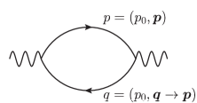
The diagrammatic representation of the connected contribution from Eq. (20) is displayed in Fig. 2, from which we can recognize that this is nothing but the diagram for the photon self-energy (polarization tensor, see Ref. [66] for discussions on the vacuum polarization in a magnetic field). Therefore the answer must be zero in the limit of zero momentum insertion from the external legs; otherwise the photon becomes massive and breaks gauge invariance. It is obvious from such a recognition that the UV divergent answer in Eq. (19) is unphysical and merely an artifact from the naive cutoff prescription.
The corresponding expression to Fig. 2 translates into the current susceptibility of our interest here given in the following form;
| (21) |
where represents the quark propagator in configuration space. Integrating over and and using the familiar expression of the propagator in momentum space for (then there is no preferred direction and so we put a subscript instead of ) we immediately reach
| (22) |
where and and . We can carry out the Matsubara frequency sum over to find,
| (23) |
Plugging the above (23) into Eq. (22) and integrating over the momentum with a UV cutoff , we can correctly rederive the result of Eq. (19) in the diagrammatic way.
Before closing this subsection we should mention on our procedure to take the limit of . In this subsection this procedure is not indispensable; we could have started the calculation with . Then, the residue of a double pole gives a term involving the derivative of the distribution functions with respect to which is exactly the same as the term arising from the limit. The reason why we distinguished from is that, as we will see shortly, the presence of induces a difference in the transverse component in Landau-quantized momenta. Thus, the calculation process elucidated in this subsection has a smooth connection to the later generalization.
3.3 Turning on — step ii)
In the presence of non-zero the transverse and longitudinal directions become distinct even before introducing finite , which should result in regardless of topological excitations. We already know the answer for the longitudinal susceptibility from Eq. (17), that is, by taking the limit of , we can readily write down,
| (24) |
Let us calculate the transverse susceptibility by means of the diagrammatic method developed in the previous subsection. For this purpose we should first come by the quark propagator under a constant magnetic field.
The solution of the Dirac equation with a constant magnetic field is known, which forms the complete set of orthogonal wave-functions. We here introduce several new notations. We use the following basis functions in a gauge choice where and ;
| (25) |
with being the standard Landau-quantized wave-function defined by
| (26) |
where represents the Hermite polynomial of degree . (We omit the subscript of for the moment.) We can easily confirm that the basis functions satisfy the orthogonality property as follows;
| (27) |
We can define the projection matrix with respect to the Dirac index according to Ritus’ method [67] as
| (28) |
for and and are swapped for the case with . It is then straightforward to prove that
| (29) |
where the right-hand side is expressed in a form of the free Dirac operator with a modified momentum . Hence, the solution of the Dirac equation with a magnetic field is given by a combination of the projection matrix and the free Dirac spinors for particles and for antiparticles with a momentum argument , that is,
| (30) |
Here we note that is a real function. Using these complete-set functions and defining associated creation and annihilation operators, we can compute the propagator to reach
| (31) |
It should be noted that and have implicit dependence in the argument (see Eq. (25)). The spin degeneracy is automatically taken into account by the property that and thus only one spin state has a non-zero contribution for .
We use this form of the quark propagator to express the susceptibility (21). Then we have to perform the coordinate integration with respect to , , , , , , , , and the momentum integration over , , , , , and also the summation over and , where , , , and are from another . As usual, after we integrate with respect to , , and , we have (there is no momentum insertion from external legs), from which only the integrations with respect to , , and remain. Then, renaming and , we have
| (32) |
where we have defined , , and . Because is now common in all , , etc, a shift in the integration variables, and , can get rid of from the integrand. Therefore, simply counts the number of Landau-quantized states, that is given by . Here is nothing but the volume . After all we can write the above into a form of
| (33) |
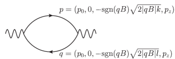
Apart from the projection operator which we will discuss soon below, this expression has a diagrammatic representation with momenta running in the loop as depicted in Fig. 3.
Because is a combination of the unit matrix and as defined in Eq. (28) and thus is commutative with , the longitudinal susceptibility is easy to evaluate. Using and the orthogonality (27), after integration over , we obtain for and for . The calculation is then reduced to the same as in the previous case with several replacements; the momentum by , and the integration with respect to transverse momenta by the summation over the Landau levels. Then the longitudinal result of Eq. (24) is almost trivially understood from Eq. (23) with .
We are now ready to consider the transverse polarization. In this case and are not commutative with . Because the calculations for and are just parallel, we focus only on the case of below. Using
| (34) |
we can evaluate the trace with respect to the Dirac index to arrive finally at
| (35) |
It should be mentioned that there emerges no spin degeneracy factor in the above expression. Taking the Matsubara sum leads to
| (36) |
with, as indicated in Fig. 3, and , where . Here we note that and are both bounded by the UV cutoff, that is, the maximum is with , and is cut off by . We realize then that subsequent terms are canceled in summation over and only the edge term (from ) remains non-vanishing, which is reminiscent of the remaining surface term in the case out of the momentum integration of Eq. (23). Therefore, at last, we get
| (37) |
after the summation with respect to from to . To be more precise, it should be mentioned here that we approximated as , which is valid as long as .
It is very interesting that we can find a simple analytical formula for the difference . From Eqs. (24) and (37) we can write,
| (38) |
where, as we have already defined, and . The point is that we can rewrite the latter term in the parentheses into a form of the discrete summation from the fact that is defined by the floor function. That is,
| (39) |
This form (times two) exactly looks like the first term in the parentheses except for the term. Therefore, only the zero-mode with contributes to the final expression;
| (40) |
Although and are divergent in the gauge-variant cutoff scheme, as we have mentioned before, the difference between them is certainly UV finite, so that it can be a well-defined quantity.
3.4 Introducing — step iii)
To treat the situation in the presence of not only but also , we need to insert the projection matrices defined as
| (41) |
to calculate the quark propagator which involves the inversion of Dirac matrices. The above-defined projection matrices have the following property,
| (42) |
We can identify as appearing in Eq. (9), so that is the projection operator to the state with helicity . We insert the unity, , after the propagator to take the inversion. By doing this we can express the susceptibility in the following way;
| (43) |
Since we know the answer for the longitudinal susceptibility, let us concentrate in calculating the transverse one (i.e. ) hereafter. After the integration over and with Eq. (34) we can find
| (44) |
where
| (45) |
We note that in the convention we are using (where ). After some lengthy calculations we can notice that becomes as simple as
| (46) |
from which we get
| (47) |
The Matsubara sum amounts to
| (48) |
Here we note that this expression consists of two parts; the former part contains the distribution function with an argument (i.e. and ) and so the summation over can be easily taken to simplify the coefficient in front of . Remarkable simplification occurs as a result of the helicity sum, which leads us to
| (49) |
From this it is apparent that there is a major cancellation in the summation with respect to and only the edge terms remain non-vanishing. Hence, we carry the summation out to find the following expression;
| (50) |
Therefore, after lengthy procedures in this subsection, what we find out at last is almost the same as Eq. (40) with a minor modification by , that is,
| (51) |
In the limit of the susceptibility difference has no dependence on .
3.5 Discussion
Since the final results are so simple, we will present another way to get the same answer from heuristic arguments. Let us consider a situation in which a homogeneous magnetic field is parallel to a homogeneous electric field . In such situation a current parallel to the magnetic field will be generated by the Schwinger process. For infinitesimal the rate of change of this current is determined by the electromagnetic anomaly relation leading to
| (52) |
We can choose a gauge so that , and then is also infinitesimally small, which allows us to use the linear response relation to express the current changing rate in another form,
| (53) |
Assuming the translational invariance in time in , we can replace acting on it by , and then we can perform the integration by parts to move acting onto which results in . Eventually we arrive at
| (54) |
Identification of the left-hand side of Eq. (52) with that of Eq. (54) concludes,
| (55) |
Now we could do the same derivation for to find that it is zero. The reason is that is always vanishing for infinitesimal in the transverse direction; small transverse electric field cannot give rise to an electric current in the transverse direction because of the energy barrier by the Landau quantization. Therefore , and so Eq. (55) gives the difference , which is in agreement with our results (40) or (51).
The anomaly equation is an exact relation. Therefore, since this derivation clearly shows that the electric-current susceptibility is determined by the electromagnetic anomaly, we conjecture that at least for massless quarks our results are exact and will not be modified by including perturbative gluonic interactions that do not affect chirality.
In Appendix B we will argue that the current susceptibility is in some sense similar to the current-chirality correlation. There, we will see that the anomaly relation again constrains the current-chirality correlation.
Our results and the above-mentioned heuristic arguments are consistent with what is known in condensed matter physics. The hall conductivity (the electric conductivity in the -direction when is imposed in the -direction) in the presence of the magnetic field is a quite familiar quantity and our and could be regarded as and in the terminology of the quantum hall effect apart from the fact that the susceptibility is a quantity in the zero-momentum limit at zero frequency, while the conductivity can be a function of finite momentum and frequency [54]. Because our calculation has three spatial dimensions, the counterpart in condensed matter physics is the multilayer Dirac electron system. Then, as discussed and confirmed in Ref. [68], only the Landau zero-mode dominates the physics properties; is zero because the transverse current operator involves a shift in the Landau level as is embodied in Eq. (34) in our calculation, which is actually a common knowledge in condensed matter physics. The longitudinal one, on the other hand, is finite and is basically given by transport from zero-mode on one layer to zero-mode on another layer. In our calculation for relativistic quark matter it is intriguing that such a finite contribution along the longitudinal direction is uniquely constrained through the exact anomaly relation.
4 Discussions on Lattice QCD and Experimental Data
Now that we have a simple expression for , it would be an interesting question whether our results are consistent with the existing results from the lattice QCD simulation [37] and from the previous work [30] aimed at describing the CME in heavy ion collisions. In this section we will see that our estimate shows reasonable agreement with lattice QCD and the formulas given in the previous work.
4.1 Lattice QCD Data
In Ref. [37] the ITEP lattice group reported on the electric-current susceptibility in quenched QCD which they found to be larger in the longitudinal direction than in the transverse direction. The simulation condition is that with , the lattice spacing (i.e. ), the volume (and thus ), and the simulation is done with . Our calculations make sense above where the physical degrees of freedom are quarks, so let us compare with the lattice results at .
First of all, plugging the above numbers into Eq. (19) we find as
| (56) |
which is much larger than the lattice result. This is not contradictory, however. As we have emphasized repeatedly in this paper, a non-zero value of is an artifact of the naive momentum cutoff, and our scheme of UV regularization is different from the lattice one.
More interesting is the comparison of the UV-finite difference , which turns out to be
| (57) |
This is fairly close to the lattice results of Ref. [37]. To make the comparison easily visible we shall compare our estimate with the lattice data corresponding to Fig. 8 in Ref. [37] for the difference between the longitudinal and transverse susceptibilities. Figure 4 plots our estimate of Eq. (57) versus the lattice QCD data. It is apparent that Eq. (57) is in good agreement within the error bars of the lattice data.
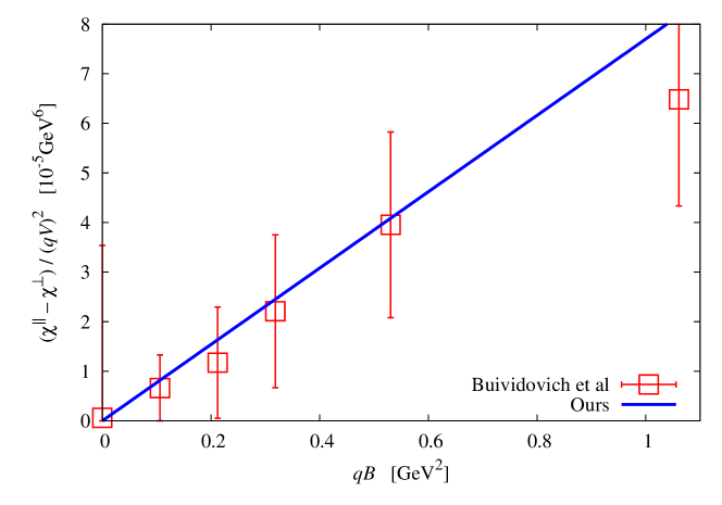
One may wonder why Eq. (57) works so well even though it does not contain any information on the topological excitations and thus no dependence on . We think that a possible explanation is the following: Euclidean lattice simulations do not describe the real-time dynamics responsible for the generation of a finite . On the other hand, the Euclidean instanton transitions (that are reproduced in lattice calculations) become suppressed in the deconfined phase, as suggested by the rapid decrease of topological susceptibility above observed on the lattice [11]. Because of this, the instantons may no longer provide a major contribution to the current susceptibility in the deconfined phase. If so, this would provide a natural explanation for the observation that the lattice results are almost independent of the magnetic field at [37]. This would also agree with the model calculation of Ref. [44] that found the CME current becoming insensitive to the magnetic field at high temperature due to the depletion of instanton effects. One can test this conjecture in lattice calculations by evaluating the susceptibility in fixed sectors of topological charge (corresponding to a highly excited QCD vacuum configuration that arguably resembles the matter produced in a heavy ion collision).
4.2 Experimental Observable
In this subsection we will check the consistency of our formula with Ref. [30]. For this purpose we shall reiterate some phenomenological discussions in Ref. [30].
Using the calculated current and susceptibility we can express the fluctuation observables as a function of the volume , the magnetic field , the chiral chemical potential , etc. That is,
| (58) |
The problem is that this expression at first sight may appear different from that discussed previously in Ref. [30]. However below we explain that the first term stemming from the CME in fact has essentially the same form as discussed in Ref. [30].
In describing the real data, it is necessary to take account of the screening effect in the direction (denoted previously as in Ref. [30]). Because emulates the effect of topologically non-trivial domains in a hot medium, it would be a reasonable interpretation that our estimate is a valid answer in each domain with a finite volume . Here, if the topological domain is characterized by a sphaleron excitation, is the typical sphaleron size.
Now the sphaleron can get excited anywhere in the medium and we should sum over all excitations. If an excitation occurs deep in a medium, it is unlikely that current fluctuations from the corresponding domain can propagate to survive outside because of medium screening. On the other hand a sphaleron excitation near the surface can easily escape from the medium, and then it should contribute to the total current fluctuations if the correlator is for same charges. In the case of opposite charges, however, as is clear from our discussions in Sec. 2, fluctuations arise from, for example, an upgoing positive charge and a downgoing negative charge. Thus, one of two charges must be significantly quenched by the medium. In Ref. [30] a phenomenological ansatz for such effects was introduced by the following functions;
| (59) | ||||
| (60) |
for the correlations with same and opposite charges, respectively, where
| (61) |
with a phenomenological screening length and
| (62) |
is the surface of matter. Here is the impact parameter, is the radius of the nucleus.
We postulate that the superposition of the sphaleron domains with over the whole system geometry amounts to the system volume factor with the quenching effect taken into account, that is, is replaced as
| (63) |
At this point let us think of the -integration. The latter term in Eq. (58) does not have any dependence, so the -integration is trivial leading to . The former term, in contrast, is proportional to . This means that after the integration turns to be a parameter (denoted as here) characterizing the dispersion of the distribution. Consequently we have the final expressions for the respective cases with the same and opposite charges;
| (64) |
and given by almost the same with replaced by in the above. Here we note that we should identify as
| (65) |
where is the sphaleron rate which is proportional to at high and thus represents how much topological excitations occur within a time slice . By the dimensional reason appears. Then we clearly see that the first term in Eq. (64) has exactly the same structure as the expression discussed in Ref. [30] apart from its overall coefficient once it is integrated over the time; . In this way we have established a relation between the formalism addressed here and the previous work in Ref. [30].
To proceed to more concrete analysis we need to specify , and as a function of (or the centrality). Although those phenomenological analyses are important, we will postpone such investigations and discuss them in a separate publication which focuses more on the phenomenology of heavy-ion collisions.
5 Summary
In this paper we formulated the Chiral Magnetic Effect in terms of the electric-current correlation function in a hot QCD medium. We computed the electric-current susceptibility in the presence of both the magnetic field and the chiral chemical potential . Because of the presence of a preferred direction fixed by , we found that the longitudinal (parallel to ) susceptibility is greater than the transverse (perpendicular to ) one . The difference arises from only the Landau zero-mode and is given by a UV-finite expression; . We also gave an intuitive derivation of our result based on the anomaly relation. We checked that our result leads to a satisfactory agreement with the electric-current susceptibility measured in the lattice QCD simulation [37].
Although has an origin in the anomaly, the expression for shows that this difference is independent of and thus is not sensitive to the real-time topological contents of the QCD matter. Therefore we should identify it as a background on top of the CME contribution stemming from the square of the induced CME current. Since the CME-induced current is proportional to and , the charge-asymmetry fluctuation relevant to the CME has a dependence of and which translates into a dispersion parameter of the -distribution; on the other hand, the non-CME term is proportional to . It would be an interesting question to check if this expected quadratic dependence on can be seen in a lattice simulation restricted to a particular topological sector of QCD, that would correspond to a highly excited vacuum configuration resembling the matter produced in a heavy ion collision.
There is an urgent need at the moment in the quantitative phenomenological approaches to CME that on one hand have a firm theoretical ground and on the other hand allow a direct comparison to the experimental data from RHIC [35]. We view the computation presented here as a necessary step towards a construction of such an approach. We will report on our approach and on the direct quantitative description of RHIC data in the forthcoming separate publication.
Acknowledgments
We thank Pavel Buividovich, Maxim Chernodub, and Mikhail Polikarpov for useful discussions and for kindly providing us with their lattice QCD data. We are grateful to Tom Blum for valuable discussions on CME with light quarks. K. F. thanks Takao Morinari for discussions in relation to condensed matter physics. The work of K. F. was supported by Japanese MEXT grant No. 20740134 and also supported in part by Yukawa International Program for Quark Hadron Sciences. The work of D. K. was supported by the Contract No. #DE-AC02-98CH10886 with the U.S. Department of Energy. The work of H.J. W. was supported by the Alexander von Humboldt Foundation.
Appendix A Appendix: Induced current from the diagrammatic method
In Refs. [31] and [54] we have discussed several different derivations of the induced current in a magnetic field in the presence of non-zero chirality. Here we add an alternative derivation using the propagator Eq. (31).
From Eq. (31) we readily obtain for the induced current along the magnetic field,
| (66) |
Since commutes with we need to evaluate the integral over of which equals for and for . Inserting the projection operators like in Eq. (43) and using Eq. (42) it can be seen that we need to evaluate the following two traces;
| (67) | |||
| (68) |
For we only need the former trace, which vanishes after integration over . The only contribution to the current comes from the latter trace when , which is the lowest Landau level. Hence we obtain after summing over Matsubara frequencies,
| (69) |
where for the Landau zero-mode. Noticing that and integrating over we obtain like in Eq. (15) the known result; , which is independent of , and .
Appendix B Appendix: Current-chirality correlation
Here we will discuss the correlation of the chirality with the current in the direction parallel to the magnetic field. We will show that the magnitude of this correlation is very similar to the difference between the longitudinal and transverse susceptibility.
By taking the derivative of Eq. (15) with respect to one can easily find the correlation between the chirality and the longitudinal current. Such a calculation immediately yields,
| (70) |
where the total chirality is the volume integral over the zero-component of the axial charge, i.e. . This correlation function shows that in a magnetic field the longitudinal current is correlated with the chirality, which is the Chiral Magnetic Effect. The magnitude of this correlation is very similar to the difference between the longitudinal and transverse susceptibility as can be inferred from Eq. (51). The only alteration comes from the charges because the chirality is not accompanied by the charge unlike the current. However, depends on the sign of , while does not.
In the same way as in Sec. 3.5 we could have also arrived at Eq. (70) using the linear response theory. In that case we start from the anomaly equation for massless particles which reads
| (71) |
Applying the same arguments as in Sec. 3.5 and replacing one with in the arguments we can recover Eq. (70) correctly.
The reason why the current-chirality correlator is so similar to the difference between the longitudinal and transverse susceptibility is that both quantities follow from the axial anomaly. This can be understood explicitly in view of the respective starting points of the linear response derivation, namely, Eq. (52) and Eq. (71).
References
- [1] A. A. Belavin, A. M. Polyakov, A. S. Shvarts and Yu. S. Tyupkin, Phys. Lett. B 59, 85 (1975).
- [2] S. L. Adler, Phys. Rev. 177, 2426 (1969); J. S. Bell and R. Jackiw, Nuovo Cim. A 60, 47 (1969).
- [3] C. G. Callan, R. F. Dashen and D. J. Gross, Phys. Lett. B 63, 334 (1976).
- [4] C. A. Baker et al., Phys. Rev. Lett. 97, 131801 (2006) [arXiv:hep-ex/0602020].
- [5] J. E. Kim and G. Carosi, arXiv:0807.3125 [hep-ph].
- [6] F. Wilczek, Phys. Rev. Lett. 40, 279 (1978).
- [7] S. Weinberg, Phys. Rev. Lett. 40, 223 (1978).
- [8] R. D. Peccei and H. R. Quinn, Phys. Rev. Lett. 38, 1440 (1977).
- [9] R. D. Peccei, Lect. Notes Phys. 741, 3 (2008) [arXiv:hep-ph/0607268].
- [10] H. Leutwyler and A. V. Smilga, Phys. Rev. D 46, 5607 (1992).
- [11] For a review including latest lattice simulations, see E. Vicari and H. Panagopoulos, Phys. Rept. 470, 93 (2009) [arXiv:0803.1593 [hep-th]].
- [12] R. F. Dashen, Phys. Rev. D 3, 1879 (1971); M. Creutz, Phys. Rev. Lett. 92, 201601 (2004) [arXiv:hep-lat/0312018]; Annals Phys. 324, 1573 (2009) [arXiv:0901.0150 [hep-ph]].
- [13] D. Boer and J. K. Boomsma, Phys. Rev. D 78, 054027 (2008) [arXiv:0806.1669 [hep-ph]]; A. J. Mizher and E. S. Fraga, Nucl. Phys. A 820, 247C (2009) [arXiv:0810.4115 [hep-ph]]; J. K. Boomsma and D. Boer, Phys. Rev. D 80, 034019 (2009) [arXiv:0905.4660 [hep-ph]].
- [14] N. S. Manton, Phys. Rev. D 28, 2019 (1983); F. R. Klinkhamer and N. S. Manton, Phys. Rev. D 30, 2212 (1984).
- [15] L. D. McLerran, E. Mottola and M. E. Shaposhnikov, Phys. Rev. D 43, 2027 (1991).
- [16] P. Arnold, D. Son and L. G. Yaffe, Phys. Rev. D 55, 6264 (1997) [arXiv:hep-ph/9609481].
- [17] P. Huet and D. T. Son, Phys. Lett. B 393, 94 (1997) [arXiv:hep-ph/9610259].
- [18] D. Bodeker, Phys. Lett. B 426, 351 (1998) [arXiv:hep-ph/9801430].
- [19] T. D. Lee, Phys. Rev. D 8, 1226 (1973).
- [20] T. D. Lee and G. C. Wick, Phys. Rev. D 9, 2291 (1974).
- [21] P. D. Morley and I. A. Schmidt, Z. Phys. C 26, 627 (1985).
- [22] D. Kharzeev, R. D. Pisarski and M. H. G. Tytgat, Phys. Rev. Lett. 81, 512 (1998) [arXiv:hep-ph/9804221];
- [23] A. A. Anselm, Phys. Lett. B 217, 169 (1989); A. A. Anselm and M. G. Ryskin, Phys. Lett. B 266 (1991) 482; J. P. Blaizot and A. Krzywicki, Phys. Rev. D 46, 246 (1992); J. D. Bjorken, K. L. Kowalski and C. C. Taylor, arXiv:hep-ph/9309235; K. Rajagopal and F. Wilczek, Nucl. Phys. B 404, 577 (1993) [arXiv:hep-ph/9303281].
- [24] D. Kharzeev and R. D. Pisarski, Phys. Rev. D 61, 111901 (2000) [arXiv:hep-ph/9906401].
- [25] S. A. Voloshin, Phys. Rev. C 62, 044901 (2000) [arXiv:nucl-th/0004042];
- [26] L. E. Finch, A. Chikanian, R. S. Longacre, J. Sandweiss and J. H. Thomas, Phys. Rev. C 65, 014908 (2002).
- [27] D. Kharzeev, Phys. Lett. B 633, 260 (2006) [arXiv:hep-ph/0406125].
- [28] D. Kharzeev and A. Zhitnitsky, Nucl. Phys. A 797, 67 (2007) [arXiv:0706.1026 [hep-ph]].
- [29] D. E. Kharzeev, arXiv:0911.3715 [hep-ph].
- [30] D. E. Kharzeev, L. D. McLerran and H. J. Warringa, Nucl. Phys. A 803, 227 (2008) [arXiv:0711.0950 [hep-ph]].
- [31] K. Fukushima, D. E. Kharzeev and H. J. Warringa, Phys. Rev. D 78, 074033 (2008) [arXiv:0808.3382 [hep-ph]].
- [32] S. A. Voloshin, Phys. Rev. C 70, 057901 (2004) [arXiv:hep-ph/0406311].
- [33] I. V. Selyuzhenkov [STAR Collaboration], Rom. Rep. Phys. 58, 049 (2006) [arXiv:nucl-ex/0510069].
- [34] S. A. Voloshin [STAR Collaboration], arXiv:0806.0029 [nucl-ex].
- [35] B. I. Abelev et al. [STAR Collaboration], arXiv:0909.1717 [nucl-ex]; arXiv:0909.1739 [nucl-ex].
- [36] F. Wang, arXiv:0911.1482 [nucl-ex].
- [37] P. V. Buividovich, M. N. Chernodub, E. V. Luschevskaya and M. I. Polikarpov, Phys. Rev. D 80, 054503 (2009) [arXiv:0907.0494 [hep-lat]]; arXiv:0909.1808 [hep-ph]; arXiv:0909.2350 [hep-ph].
- [38] M. Abramczyk, T. Blum, G. Petropoulos and R. Zhou, arXiv:0911.1348 [hep-lat].
- [39] G. Lifschytz and M. Lippert, Phys. Rev. D 80, 066007 (2009) [arXiv:0906.3892 [hep-th]]; Phys. Rev. D 80, 066005 (2009) [arXiv:0904.4772 [hep-th]].
- [40] H. U. Yee, JHEP 0911, 085 (2009) [arXiv:0908.4189 [hep-th]].
- [41] A. Rebhan, A. Schmitt and S. A. Stricker, arXiv:0909.4782 [hep-th].
- [42] B. Sahoo and H. U. Yee, arXiv:0910.5915 [hep-th].
- [43] E. D’Hoker and P. Kraus, arXiv:0911.4518 [hep-th].
- [44] S. i. Nam, arXiv:0911.0509 [hep-ph]; arXiv:0912.1933 [hep-ph].
- [45] R. Millo and P. Faccioli, Phys. Rev. D 77, 065013 (2008) [arXiv:0706.0805 [hep-ph]].
- [46] E. S. Fraga and A. J. Mizher, Phys. Rev. D 78, 025016 (2008) [arXiv:0804.1452 [hep-ph]]; arXiv:0810.5162 [hep-ph].
- [47] T. D. Cohen, D. A. McGady and E. S. Werbos, Phys. Rev. C 76, 055201 (2007) [arXiv:0706.3208 [hep-ph]].
- [48] D. P. Menezes, M. Benghi Pinto, S. S. Avancini, A. Perez Martinez and C. Providencia, Phys. Rev. C 79, 035807 (2009) [arXiv:0811.3361 [nucl-th]]; D. P. Menezes, M. Benghi Pinto, S. S. Avancini and C. Providencia, arXiv:0907.2607 [nucl-th].
- [49] V. Skokov, A. Illarionov and V. Toneev, arXiv:0907.1396 [nucl-th].
- [50] V. A. Okorokov, arXiv:0908.2522 [nucl-th].
- [51] A. A. Andrianov and D. Espriu, Phys. Lett. B 663, 450 (2008) [arXiv:0709.0049 [hep-ph]].
- [52] M. A. Metlitski and A. R. Zhitnitsky, Nucl. Phys. B 731, 309 (2005) [arXiv:hep-ph/0508004].
- [53] A. Parnachev and A. R. Zhitnitsky, Phys. Rev. D 78, 125002 (2008) [arXiv:0806.1736 [hep-ph]].
- [54] D. E. Kharzeev and H. J. Warringa, Phys. Rev. D 80, 034028 (2009) [arXiv:0907.5007 [hep-ph]].
- [55] S. A. Voloshin [STAR Collaboration], arXiv:0907.2213 [nucl-ex].
- [56] M. A. Stephanov, K. Rajagopal and E. V. Shuryak, Phys. Rev. Lett. 81, 4816 (1998) [arXiv:hep-ph/9806219]; Phys. Rev. D 60, 114028 (1999) [arXiv:hep-ph/9903292].
- [57] P. Arnold and L. D. McLerran, Phys. Rev. D 37, 1020 (1988).
- [58] D. Y. Grigoriev, V. A. Rubakov and M. E. Shaposhnikov, Nucl. Phys. B 326, 737 (1989).
- [59] J. Ambjorn, T. Askgaard, H. Porter and M. E. Shaposhnikov, Phys. Lett. B 244, 479 (1990); J. Ambjorn, T. Askgaard, H. Porter and M. E. Shaposhnikov, Nucl. Phys. B 353, 346 (1991).
- [60] G. D. Moore, C. r. Hu and B. Muller, Phys. Rev. D 58, 045001 (1998) [arXiv:hep-ph/9710436]; G. D. Moore and K. Rummukainen, Phys. Rev. D 61, 105008 (2000) [arXiv:hep-ph/9906259]; D. Bodeker, G. D. Moore and K. Rummukainen, Phys. Rev. D 61, 056003 (2000) [arXiv:hep-ph/9907545].
- [61] E. Meggiolaro, Phys. Rev. D 58, 085002 (1998) [arXiv:hep-th/9802114].
- [62] D. Kharzeev, A. Krasnitz and R. Venugopalan, Phys. Lett. B 545, 298 (2002) [arXiv:hep-ph/0109253].
- [63] A. Y. Alekseev, V. V. Cheianov and J. Frohlich, Phys. Rev. Lett. 81, 3503 (1998) [arXiv:cond-mat/9803346].
- [64] M. A. Metlitski and A. R. Zhitnitsky, Phys. Rev. D 72, 045011 (2005) [arXiv:hep-ph/0505072].
- [65] G. M. Newman and D. T. Son, Phys. Rev. D 73, 045006 (2006) [arXiv:hep-ph/0510049].
- [66] W. y. Tsai, Phys. Rev. D 10, 2699 (1974).
- [67] V. I. Ritus, Annals Phys. 69 (1972) 555; C. N. Leung, Y. J. Ng and A. W. Ackley, Phys. Rev. D 54, 4181 (1996); E. Elizalde, E. J. Ferrer and V. de la Incera, Annals Phys. 295, 33 (2002) [arXiv:hep-ph/0007033]; E. J. Ferrer, V. de la Incera and C. Manuel, Nucl. Phys. B 747, 88 (2006) [arXiv:hep-ph/0603233].
- [68] T. Osada, J. Phys. Soc. Jpn. 77, 084711 (2008); N. Tajima et al., Phys. Rev. Lett. 102, 176403 (2009).