Nonlocal Potentials and
Complex Angular Momentum Theory

Abstract

The purpose of this paper is to establish meromorphy properties of the partial scattering amplitude $T(\lambda,k)$ associated with physically relevant classes $\mathcal{N}_{w^{(\varepsilon)}\!,\alpha}^{\,\gamma}$ of nonlocal potentials in corresponding domains $D_{\gamma,\alpha}^{(\delta)}$ of the space $\mathbb{C}^{2}$ of the complex angular momentum $\lambda$ and of the complex momentum $k$ (namely, the square root of the energy). The general expression of $T$ as a quotient $\Theta(\lambda,k)/\sigma(\lambda,k)$ of two holomorphic functions in $D_{\gamma,\alpha}^{(\delta)}$ is obtained by using the Fredholm–Smithies theory for complex $k$, at first for $\lambda=\ell$ integer, and in a second step for $\lambda$ complex ($\mathop{\mathrm{Re}}\lambda>-1/2$). Finally, we justify the “Watson resummation” of the partial wave amplitudes in an angular sector of the $\lambda$–plane in terms of the various components of the polar manifold of $T$ with equation $\sigma(\lambda,k)=0$. While integrating the basic Regge notion of interpolation of resonances in the upper half–plane of $\lambda$, this unified representation of the singularities of $T$ also provides an attractive possible description of antiresonances in the lower half–plane of $\lambda$. Such a possibility, which is forbidden in the usual theory of local potentials, represents an enriching alternative to the standard Breit–Wigner hard–sphere picture of antiresonances.

1 Introduction

In the standard Breit–Wigner theory of scattering the notions of “time delay” and “time advance”, corresponding respectively to the increasing or decreasing character of a given phase–shift as a function of the energy (see, e.g., [1, pp. 110 and 111]) are not described in a symmetric way: while the former is described by a pole singularity of the scattering amplitude, the latter relies on the model of scattering by an impenetrable sphere. A question then arises: can the time advance still be evaluated in terms of hard–sphere scattering in collisions between composite particles, when Pauli exclusion principle comes into play? We recall, indeed, that when two composite particles collide, the fermionic character of the components emerges and the antisymmetrization of the whole system generates repulsive exchange–forces, which can produce antiresonances, and are thus responsible for the occurrence of time advance.

From a more formal viewpoint, if antiresonances can be defined in a way which parallels the description of resonances, namely as bumps in the energy–dependance plot of the cross–section associated with the downward (instead of upward) passage through $\frac{\pi}{2}$ of a given phase–shift, their status has remained rather obscure in terms of the analyticity properties in energy of the scattering functions, in comparison with the success of the standard pole–resonance conceptual correspondance. The reason for this discrepancy lies in the fact that the Breit–Wigner poles associated with resonances necessarily occur in the “second–sheet” of the energy variable $E$, namely in the lower half–plane of the usual momentum variable $k=\sqrt{E}$, near the positive real axis; this is a situation which readily accounts for the upward passage of the phase–shift through $\frac{\pi}{2}$. But then the natural candidacy of poles in the upper half–plane for accounting the downward passage characterizing the antiresonances turns out to be strictly forbidden in any formalism of scattering theory (as well in nonrelativistic potential theory as in relativistic quantum field theory) as a constraint imposed by the causality principle. However one also knows that for any given phase–shift the antiresonances are present together with the resonances. In fact, the physically observed occurrence of resonance–antiresonance pairs finds its firm theoretical basis in the Levinson theorem (see [1, p. 206]) which prescribes the equality of each phase–shift at zero and infinite energies in the absence of bound states.

Considering the present sum of knowledge that is available in the general theory of quantum scattering processes, it seems to us that there remains a problem of global understanding of the organization of sequences of resonances and associated antiresonances for successive values of the angular momentum $\ell$ and of the corresponding relationships between the energy variable $E$ (or $k$) and $\ell$. Let us recall the historical situation from both theoretical and experimental aspects. At first, the standard theory of scattering does not attempt to group resonances in families: each resonance is simply described by a fixed pole singularity in the energy variable. As for antiresonances, they are individually parametrized in a very rough way and from the outset by the hard–sphere picture. However, phenomenological data clearly show that the resonances often appear in ordered sequences, such as rotational bands. Typical examples can be observed in $\alpha$–$\alpha$, $\alpha$–⁴⁰Ca, ¹²C–¹²C, ²⁸Si–²⁸Si, and other heavy–ion collisions (see [2] and references quoted therein). In these examples, the resonances are ordered in rotational bands of levels whose energy spectrum can be fitted by an expression of the form $E_{\ell}=A+B\ell(\ell+1)$, where $\ell$ is the angular momentum of the level, and $A$ and $B$ are constants. Furthermore, the widths of the resonances increase as a function of the energy.

Since 1960, a wide opening on the previous problem was given by Regge’s basic formalism of the holomorphic interpolation of scattering partial waves in the complex angular momentum (CAM) variable $\lambda$ (see [3]). In this formalism, the concept of pole reached his full fecondity through the association of sequences of resonances with polar manifolds $\lambda=\lambda(k)$ in the complex space $\mathbb{C}^{2}$ of the variables $(\lambda,k)$. Each such polar manifold gives rise to a “trajectory” on which a sequence of complex energy values $k_{\ell}$ with $\mathop{\mathrm{Im}}k_{\ell}<0$ satisfying the equation $\lambda(k_{\ell})=\ell$ corresponds to a sequence of resonances. In view of the complex geometrical framework, a new possibility offered by that description was the study of the trajectories $\lambda=\lambda(k)$ for $k$ real and positive, realized as curves in the complex upper half–plane of $\lambda$. Coming back to the general problem that we have raised above, it now seems interesting to inquire whether this enlarged framework of complex geometry in the CAM and energy variables might give some new insight on the description of antiresonances and also on their global organization. In other words, are there some polar manifolds $\lambda=\lambda(k)$ which have something to do with the description of antiresonances?

A tentative answer to this question was proposed by various authors (see [4]) by considering in particular the case of scattering by Yukawa–type potentials. In such cases each pole trajectory in the upper half–plane of $\lambda$ behaves as follows. After having traveled forward (i.e., with $\mathrm{d}\mathop{\mathrm{Re}}\lambda/\mathrm{d}k>0$) and described thereby a sequence of resonances at $\mathop{\mathrm{Re}}\lambda(k)=\ell$, it starts going up and turning backwards, and then passes again but in decreasing order (and with larger values of $\mathop{\mathrm{Im}}\lambda$) through points whose real parts $\mathop{\mathrm{Re}}\lambda=\ell$ had been previously visited. It was then proposed that this second part of such trajectories be associated with antiresonances. However it turns out that such a global ordering is inconsistent with most of the experimental data, which exhibit the alternance of resonances and antiresonances for successive values of $\ell$ when one follows the increase of the energy variable. From a formal viewpoint, a scenario which would appear to be much more appropriate would be the suitable coupling of a pure resonance trajectory in the upper half–plane with a pure antiresonance trajectory in the lower half–plane $\mathop{\mathrm{Im}}\lambda<0$. However, this latter possibility has been excluded from the whole theory of local potentials by a theorem proved by Regge (see [3]).

It is at this point of our considerations that we wish to advocate for the necessity of enlarging the framework of Schrödinger theory so as to include the occurrence of nonlocal potentials $V(\boldsymbol{R},\boldsymbol{R}^{\prime})$ and thereby invalidate the application of Regge’s no–go theorem. As a matter of fact, whenever the antiresonances are generated by exchange forces due to Pauli’s exclusion principle, the many–body structure of the colliding particles is involved and leads one to introduce nonlocal potentials. This class of potentials has been indeed considered long time ago, mainly in connection with the theory of nuclear matter [5, 6]. The procedures commonly used for treating the many–body dynamics, like the resonating group method [7], the complex generator coordinate technique [8], the cluster coordinate method [9], all lead to an extension of the standard Schrödinger equation, which now becomes an integro–differential equation of the same form as that obtained in the study of the nonlocal potentials. In this paper, we intend to study the singularities of the partial scattering amplitude for appropriate classes of nonlocal potentials, both in the complex momentum $k$–plane and in the complex angular momentum $\lambda$–plane. Concerning the possible location of these singularities, one of the results that we have obtained is a modified extension of the previous Regge theorem to the case of nonlocal potentials, which now opens the way to singularities in the lower half–plane of $\lambda$ (at $k$ real and positive). For local potentials (notably, Yukawian potentials) all the singularities of the partial scattering function, such as those which manifest themselves as resonances, must be located at $k>0$ in the region $\mathop{\mathrm{Im}}\lambda>0$. Here we have considered as an example a class of nonlocal potentials $V(\lambda;R,R^{\prime})=V_{*}(R,R^{\prime}){\tilde{F}}(\lambda)$, where ${\tilde{F}}(\lambda)$ is a function holomorphic, bounded, and of Hermitian–type in the half–plane $\mathbb{C}^{+}_{-\frac{1}{2}}\doteq\{\lambda\in\mathbb{C}\,:\,\mathop{\mathrm{Re}}\lambda>-\frac{1}{2}\}$. For such a class of potentials, we denote by $\mathcal{L}_{j}$ ($j\in\mathbb{Z}$) the set of lines in $\mathbb{C}^{+}_{-\frac{1}{2}}$ where $\mathop{\mathrm{Im}}{\tilde{F}}(\lambda)=0$. All the points of a curve $\mathcal{L}_{j}$ with $j>0$ (resp., $j<0$) belong to the region $\mathop{\mathrm{Im}}\lambda>0$ (resp., $\mathop{\mathrm{Im}}\lambda<0$), $\mathcal{L}_{0}$ being along the real positive axis. We prove that no singular pairs $(\lambda,k)$ can occur with $\lambda$ in any line $\mathcal{L}_{j}$ in the lower half–plane ($j\leqslant 0$), and with $\mathop{\mathrm{Im}}k>0$ and $\mathop{\mathrm{Re}}k>0$. But there is a possible occurrence of singular manifolds containing branches in the region $\mathop{\mathrm{Im}}k\geqslant 0$, $\mathop{\mathrm{Re}}k\geqslant 0$ and $\mathop{\mathrm{Re}}\lambda>0$, $\mathop{\mathrm{Im}}\lambda<0$, always located in strips of the fourth quadrant of the $\lambda$–plane, well separated from one another by the set of lines $\mathcal{L}_{j}$ ($j\leqslant 0$). These strips therefore set the ground for possible antiresonance trajectories. Although it is still premature to conclude on the existence of the latter before some numerical exploration be performed, we think that this promising result may suggest how to fill a gap between phenomenological and theoretical analysis of scattering data. Indeed, in refs. [10, 11] two of us have performed an extensive phenomenological analysis, fitting the scattering data of $\alpha$–$\alpha$ and $\pi^{+}$–p elastic scattering by using two pole trajectories in the CAM–plane. The resonances have been described by poles in the first quadrant, the antiresonances by poles in the fourth quadrant.

As a further possible motivation to the investigation of the theory of nonlocal potentials, we remind the reader that in a parallel presentation of the two–particle scattering theory in Schrödinger wave–mechanics and in Quantum Field Theory (QFT), it is a suitable Bethe–Salpeter–type kernel which plays the role of the potential [12], provided the latter be understood as a generalized potential of nonlocal–type (and also energy–dependent). Recently, the CAM formalism has been introduced in QFT [13], and it has been used to obtain a corresponding CAM–diagonalization of the Bethe–Salpeter equation [14]. Therefore, also from this viewpoint, exploring the CAM–singularities generated by appropriate classes of nonlocal potentials deserves some interest. One can even suggest that the possible occurrence of antiresonances in a QFT with baryon and meson fields, associated with composite particles (with respect to the elementary level of quark–structure), could be described in the Bethe–Salpeter framework, as a natural relativistic QFT extension of the phenomena permitted by nonlocal potential theory.

As far as we know, the connection between nonlocal potentials and complex angular momentum theory is totally missing in the literature. Let us quote what is written in the classical textbook by De Alfaro and Regge [3] on this question: “Our philosophy in regard to these potentials (i.e., nonlocal potentials) is the following: maybe they are there, but if they are there we do not know what to do with them. They will not be discussed in this book anymore.” Even in excellent texts on scattering theory, like the one by Reed and Simon [15], this problem has not been considered at all. Long time ago, one of the authors, in collaboration with others, treated the scattering theory for large classes of nonlocal potentials in a series of papers [16], where, however, the analysis in the CAM–plane was not considered. The present paper can be regarded as a continuation and completion of these works, in particular of [16, IV] (which in Section 2 is referred to as I). So, before considering the interesting problem of describing resonances and antiresonances, which will be outlined in the last section of this paper, one needs to settle on a firm basis the whole theory of scattering functions with respect to the complex variables $(\lambda,k)$ in the framework of appropriate classes of nonlocal potentials.

The paper is organized as follows: in Section 2 we recall the spectral properties associated with the Schrödinger two–particle operators for a large class of potentials $U$, which include a local part called $V_{0}$ and a nonlocal part called $V$. All these properties concern bound states and scattering solutions, and are treated in the complex half–plane $\mathop{\mathrm{Im}}k\geqslant 0$. In Section 3 we study a class $\mathcal{N}_{w,\alpha}$ of rotationally invariant nonlocal potentials $V$, which is characterized by a positive parameter $\alpha$; for such a class the previous treatment is extended to the half–plane $\mathop{\mathrm{Im}}k\geqslant-\alpha$, so as to include the analysis of resonances. In this section we use Smithies’ theory [17] of Fredholm–type integral equations for studying various properties of the resolvent when $k$ belongs to the half–plane $\{k\in\mathbb{C}:\mathop{\mathrm{Im}}k\geqslant-\alpha\}$ and the angular momentum $\ell$ is a non–negative integer. The Smithies formalism produces modified Fredholm formulae, whose advantage is to fit rigorously with the convenient framework of Hilbert–Schmidt–type kernels. It is therefore in this formalism that we investigate in detail bound states, spurious bound states (or bound states embedded in the continuum), anti–bound states, resonances, scattering solutions, and partial scattering amplitudes in the strip $\Omega_{\alpha}=\{k\in\mathbb{C}:|\mathop{\mathrm{Im}}k|<\alpha\}$. In Section 4 we study the interpolation of the so–called partial potentials (i.e., the coefficients of the Fourier–Legendre expansion of the potentials) in the plane of the complexified angular momentum variable $\lambda$. The potentials which admit this interpolation and satisfy an exponential decrease of the form $e^{-\gamma\mathop{\mathrm{Re}}\lambda}$ ($\gamma>0$) in $\mathbb{C}^{+}_{-\frac{1}{2}}$ will be called “Carlsonian potentials with CAM–interpolation $V(\lambda;R,R^{\prime})$ and rate of decrease $\gamma$”, in view of the fact that the uniqueness of the interpolation is guaranteed by Carlson’s theorem. The class of such potentials which belong to $\mathcal{N}_{w,\alpha}$ will be denoted $\mathcal{N}_{w,\alpha}^{\,\gamma}$. Then, by using the bounds on the complex angular momentum Green function (i.e., the extension of the Green function from integral non–negative values of the angular momentum $\ell$ to complex values $\lambda$) one can extend the Fredholm–Smithies formalism of the previous section in terms of vector–valued and operator–valued holomorphic functions of the two complex variables $\lambda$ and $k$. Correspondingly, one then studies the properties of the partial scattering amplitude $T(\lambda,k)$ as a meromorphic function of $\lambda$ and $k$ in appropriate domains $D_{\gamma,\alpha}^{(\delta)}$ of the space $\mathbb{C}^{2}$. This sets the basis for analyzing the notions of resonances and of antiresonances in terms of the polar singularities of $T$ in either part $\mathop{\mathrm{Im}}\lambda\gtrless 0$ of the domain $D_{\gamma,\alpha}^{(\delta)}$. The first part of Section 5 is devoted to the Watson resummation of the partial wave amplitudes in an angular sector of the complex $\lambda$–plane for all positive values of $k$ (and also in some domain of the complex $k$–plane). In the second part of this section, the notion of a dominant pole in the Watson representation of the scattering amplitude is introduced and a symmetric analysis of resonances and antiresonances is proposed in this framework. Finally, in order to make simpler the presentation of our results, we have reserved two appendices for mathematical ingredients to be used in the text: while Appendix A is devoted to the derivation of bounds on the complex angular momentum Green function and on the Bessel and Hankel functions, Appendix B deals with continuity and holomorphy properties of vector–valued and operator–valued functions.

2 A review of spectral properties for a class of Schrödinger two–particle operators including local and nonlocal potentials

We consider Schrödinger operators of the following form:

$$(H\psi)(\boldsymbol{x})=-\Delta\psi(\boldsymbol{x})+(U\psi)(\boldsymbol{x})=-\Delta\psi(\boldsymbol{x})+V_{0}(\boldsymbol{x})\psi(\boldsymbol{x})+\int V(\boldsymbol{x},\boldsymbol{y})\psi(\boldsymbol{y})\,\mathrm{d}\boldsymbol{y},$$ (2.1)

where $\boldsymbol{x}=(x_{1},x_{2},x_{3})$ is a three–dimensional real vector, $|\boldsymbol{x}|^{2}=\sum_{k=1}^{3}x_{k}^{2}$, $\Delta=\sum_{k=1}^{3}\partial^{2}/\partial x_{k}^{2}$ is the Laplace operator, and integration is on the whole $\mathbb{R}^{3}$ space. The integro–differential operator $H$ represents, in the center of mass system, the energy operator of two particles interacting through a local plus a nonlocal potential. Our assumptions on the potential functions $V_{0}$ and $V$ are the following:

• $V_{0}$ and $V$ are real–valued; $V$ is symmetric: i.e., $V(\boldsymbol{x},\boldsymbol{y})=V(\boldsymbol{y},\boldsymbol{x})$.

• $\displaystyle A_{p}=\left[\int(1+|\boldsymbol{x}|)^{p}\ |V_{0}(\boldsymbol{x})|^{p}\,\mathrm{d}\boldsymbol{x}\right]^{1/p}<+\infty\qquad(p=1,2)$.

• $\displaystyle B_{p}=\left[\int(1+|\boldsymbol{x}|)^{p}\left(\int|V(\boldsymbol{x},\boldsymbol{y})|\,\mathrm{d}\boldsymbol{y}\right)^{p}\,\mathrm{d}\boldsymbol{x}\right]^{1/p}<+\infty\qquad(p=1,2)$.

Note that condition (a) guarantees that the operator $H$ is a time–reversal invariant and formally Hermitian operator. We then have (see I):

Proposition 2.1.

If conditions (a), (b) and (c) hold, then the operator $H$ defined by (2.1) is self–adjoint in $L^{2}$ with domain $\mathcal{D}_{H}=W^{2,2}$.

In this section $L^{2}$ and $W^{2,2}$ will indicate $L^{2}(\mathbb{R}^{3})$ and $W^{2,2}(\mathbb{R}^{3})$, respectively; moreover, we recall that $W^{2,2}$ is the Sobolev space of all the square integrable functions which have square integrable distributional derivatives up to the second order.

We now consider the following problems.

Problem 1 (Bound state problem).

Suppose that the potential functions $V_{0}$ and $V$ satisfy conditions (a), (b), and (c), then we study the solutions $\psi$ with

$$\psi\in W^{2,2}\quad\mathrm{and}\quad\|\psi\|_{L^{2}}=1,$$ (2.2)

of the Schrödinger equation $(H\psi)(\boldsymbol{x})=k^{2}\psi(\boldsymbol{x})$, namely:

$$\Delta\psi(\boldsymbol{x})+k^{2}\psi(\boldsymbol{x})=(U\psi)(\boldsymbol{x})=V_{0}(\boldsymbol{x})\psi(\boldsymbol{x})+\int V(\boldsymbol{x},\boldsymbol{y})\,\psi(\boldsymbol{y})\,\mathrm{d}\boldsymbol{y},$$ (2.3)

where $k$ is a complex number with $\mathop{\mathrm{Im}}k\geqslant 0$.

The following theorem can then be proved.

Theorem 2.2.

Let $B$ be the set of values of $k$ $(\mathop{\mathrm{Im}}k\geqslant 0)$ such that a non trivial solution of Problem 1 exists; then:

• for any $k\in B$ the number of linearly independent solutions of Problem 1 (i.e., the multiplicity of $k$) is finite;

• $B$ is contained in the union of the real axis and the positive imaginary axis;

• $B$ is bounded;

• $B$ is countable with no limit points except $k=0$;

• if a real value of $k$ belongs to $B$, then $(-k)\in B$ and Problem 1 has precisely the same solutions associated with $k$ and $-k$.

Proof.

See I (proof of Theorem 2.1). ∎

We introduce the index $n$ ($n=1,2,3,\ldots$) to label the imaginary and the positive real values of $k$ which belong to $B$, and we understand to count any such value of $k$ as many times as its multiplicity. Then the numbers $E_{n}=k_{n}^{2}$ ($n=1,2,3,\ldots$) are the eigenvalues of the operator $H=-\Delta+U$; with each eigenvalue $E_{n}$ we can associate one and only one solution $\psi_{n}(\boldsymbol{x})$ of Problem 1, i.e., an eigenfunction of $H$. Since the operator $H$ is self–adjoint (see Proposition 2.1), the functions $\psi_{n}(\boldsymbol{x})$ can be regarded as forming an orthonormal system.

Problem 2 (Scattering problem).

We study solutions $\Psi_{\boldsymbol{\xi}}(\boldsymbol{x})$ of the Schrödinger equation $(H\Psi_{\boldsymbol{\xi}})(\boldsymbol{x})=|{\boldsymbol{\xi}}|^{2}\Psi_{\boldsymbol{\xi}}(\boldsymbol{x})$, which are of the following form:

$$\Psi_{\boldsymbol{\xi}}(\boldsymbol{x})=e^{\mathrm{i}\langle{\boldsymbol{\xi}},\boldsymbol{x}\rangle}+\Phi({\boldsymbol{\xi}},\boldsymbol{x}),$$ (2.4)

where ${\boldsymbol{\xi}}=(\xi_{1},\xi_{2},\xi_{3})$ is a given three–dimensional vector, $\langle{\boldsymbol{\xi}},\boldsymbol{x}\rangle=\sum_{j=1}^{3}\xi_{j}x_{j}$ and $\Phi({\boldsymbol{\xi}},\boldsymbol{x})$ satisfies the following properties:

• $\Phi({\boldsymbol{\xi}},\cdot)\in W^{2,2}_{\mathrm{loc}}$;

• $\displaystyle\Phi({\boldsymbol{\xi}},\boldsymbol{x})=O\left(\frac{1}{|\boldsymbol{x}|}\right)\qquad(|\boldsymbol{x}|\to+\infty)$;

• $\displaystyle\int_{|\boldsymbol{x}|=r}\left|\frac{\partial\Phi}{\partial|\boldsymbol{x}|}({\boldsymbol{\xi}},\boldsymbol{x})-\mathrm{i}|{\boldsymbol{\xi}}|\Phi({\boldsymbol{\xi}},\boldsymbol{x})\right|^{2}\mu(\mathrm{d}\boldsymbol{x})\xrightarrow[r\to+\infty]{}0$, $\mu$ denoting the Lebesgue measure on the sphere;

• $\displaystyle\Delta\Phi({\boldsymbol{\xi}},\boldsymbol{x})+|{\boldsymbol{\xi}}|^{2}\Phi({\boldsymbol{\xi}},\boldsymbol{x})=V_{0}(\boldsymbol{x})\Phi({\boldsymbol{\xi}},\boldsymbol{x})+\int V(\boldsymbol{x},\boldsymbol{y})\Phi({\boldsymbol{\xi}},\boldsymbol{y})\,\mathrm{d}\boldsymbol{y}+V_{0}(\boldsymbol{x})e^{\mathrm{i}\langle{\boldsymbol{\xi}},\boldsymbol{x}\rangle}$
        $\displaystyle+\int V(\boldsymbol{x},\boldsymbol{y})e^{\mathrm{i}\langle{\boldsymbol{\xi}},\boldsymbol{y}\rangle}\,\mathrm{d}\boldsymbol{y}$,  (Schrödinger equation written in terms of $\Phi$).

Note that $\Phi\in W^{2,2}_{\mathrm{loc}}$ means that $f\,\Phi\in W^{2,2}$ for any $f\in C_{0}^{\infty}(\mathbb{R}^{3})$. Besides, we remark that the third condition involves the notion of trace in the sense of Sobolev of the function $\Phi$ and of its first derivatives. To this purpose, let us note that if $u\in W^{2,2}$ and $\Sigma$ is a smooth surface, then the trace of $u$ on $\Sigma$ can be defined as the restriction of $u$ on $\Sigma$. This definition is meaningful because $u$ is a continuous function, but in the case of the first derivatives, the previous definition breaks down. However, the linear operator relating every $\Phi\in C^{\infty}_{0}(\mathbb{R}^{3})$ to $\partial\Phi/\partial x_{k}$, restricted on the sphere of radius $r$, is a continuous mapping of a subspace of $W^{2,2}$ into the space of the functions which are square integrable on the sphere of radius $r$. Since $C^{\infty}_{0}(\mathbb{R}^{3})$ is dense in $W^{2,2}$, this operator can be extended in a unique way to the whole $W^{2,2}$ (see the Appendix of I). Furthermore, any function $\Phi\in W^{2,2}_{\mathrm{loc}}$ is continuous (Lemma A.3 of I), so that from the second condition of Problem 2 it follows that $\Psi_{\boldsymbol{\xi}}$ is a bounded and continuous function of $\boldsymbol{x}$ in $\mathbb{R}^{3}$. Then the following theorem holds.

Theorem 2.3.

For any ${\boldsymbol{\xi}}\in\mathbb{R}^{3}$, ${\boldsymbol{\xi}}\not=0$, a solution of Problem 2 exists. The solution is unique if and only if $|{\boldsymbol{\xi}}|\not\in B$ (the set defined in Theorem 2.2). Any solution of Problem 2 has the following asymptotic behavior:

$$\Phi({\boldsymbol{\xi}},\boldsymbol{x}) =\frac{e^{\mathrm{i}|{\boldsymbol{\xi}}||\boldsymbol{x}|}}{|\boldsymbol{x}|}F\left(|{\boldsymbol{\xi}}|\frac{\boldsymbol{x}}{|\boldsymbol{x}|},{\boldsymbol{\xi}}\right)+o\left(\frac{1}{|\boldsymbol{x}|}\right)\qquad(|\boldsymbol{x}|\to+\infty),$$

$$F(\boldsymbol{x},{\boldsymbol{\xi}}) =-\frac{1}{4\pi}\int e^{-\mathrm{i}\langle\boldsymbol{x},\boldsymbol{y}\rangle}\left(U\Psi_{\boldsymbol{\xi}}\right)(\boldsymbol{y})\,\mathrm{d}\boldsymbol{y}.$$

The quantity $F\left(|{\boldsymbol{\xi}}|\frac{\boldsymbol{x}}{|\boldsymbol{x}|},{\boldsymbol{\xi}}\right)$, the so–called scattering amplitude, is uniquely defined for any ${\boldsymbol{\xi}}\in\mathbb{R}^{3}$.

Proof.

See I (proof of Theorem 2.2). ∎

Besides, let $\Omega^{R}$ be the set of vectors ${\boldsymbol{\xi}}\in\mathbb{R}^{3}$ such that $|{\boldsymbol{\xi}}|\not\in B$, ${\boldsymbol{\xi}}\neq 0$; then the functions $\Omega^{R}\ni{\boldsymbol{\xi}}\mapsto\Phi({\boldsymbol{\xi}},\boldsymbol{x})$ are equicontinuous, i.e.:

$$\sup_{\boldsymbol{x}\in\mathbb{R}^{3}}\left|\Phi({\boldsymbol{\xi}},\boldsymbol{x})-\Phi({\boldsymbol{\eta}},\boldsymbol{x})\right|\longrightarrow 0,$$ (2.5)

where ${\boldsymbol{\xi}}\in\Omega^{R}$ is fixed, and $|{\boldsymbol{\xi}}-{\boldsymbol{\eta}}|\to 0$.

We can rapidly sketch the approach to Problems 1 and 2. One first introduces the following operator $L(k)$:

$$L(k)f(\boldsymbol{x})=-\int\!V_{0}(\boldsymbol{x})\frac{e^{\mathrm{i}k|\boldsymbol{x}-\boldsymbol{y}|}}{4\pi|\boldsymbol{x}-\boldsymbol{y}|}f(\boldsymbol{y})\,\mathrm{d}\boldsymbol{y}-\int\!\left(\int\!V(\boldsymbol{x},\boldsymbol{z})\frac{e^{\mathrm{i}k|\boldsymbol{z}-\boldsymbol{y}|}}{4\pi|\boldsymbol{z}-\boldsymbol{y}|}\,d\boldsymbol{z}\right)\,f(\boldsymbol{y})\,\mathrm{d}\boldsymbol{y},$$ (2.6)

acting on the Hilbert space $X^{2}$ defined by

$$X^{2}=\left\{f\in L^{2}\,:\,\|f\|_{X^{2}}\doteq\left(\int(1+|\boldsymbol{x}|)^{2}|f(\boldsymbol{x})|^{2}\,\mathrm{d}\boldsymbol{x}\right)^{1/2}<+\infty\right\}.$$

Note that the function ${e^{\mathrm{i}k|\boldsymbol{x}-\boldsymbol{y}|}}/{4\pi|\boldsymbol{x}-\boldsymbol{y}|}$ (in definition (2.6) of the operator $L(k)$), is the Green function associated with the classical radiation problem. Next, one applies the Riesz–Schauder theory [18] to the resolvent $R(k)=[1-L(k)]^{-1}$, and then the following alternative holds:

• either $R(k)=[1-L(k)]^{-1}$ exists and is a bounded operator on $X^{2}$;

• or the space spanned by the eigenfunctions of $L(k)$ has dimension $n\geqslant 1$.

In case (a) the integral equation

$$v({\boldsymbol{\xi}},\cdot)=v_{0}({\boldsymbol{\xi}},\cdot)+L(|{\boldsymbol{\xi}}|)\,v({\boldsymbol{\xi}},\cdot),$$ (2.7)

where

$$v_{0}({\boldsymbol{\xi}},\boldsymbol{x})=V_{0}(\boldsymbol{x})\,e^{\mathrm{i}\langle{\boldsymbol{\xi}},\boldsymbol{x}\rangle}+\int V(\boldsymbol{x},\boldsymbol{y})\,e^{\mathrm{i}\langle{\boldsymbol{\xi}},\boldsymbol{y}\rangle}\,\mathrm{d}\boldsymbol{y},$$

has a unique solution in $X^{2}$, i.e.:

$$v({\boldsymbol{\xi}},\cdot)=R(|{\boldsymbol{\xi}}|)\,v_{0}({\boldsymbol{\xi}},\cdot).$$

In case (b), Eq. (2.7) has a solution $v({\boldsymbol{\xi}},\cdot)\in X^{2}$ if and only if $v_{0}({\boldsymbol{\xi}},\cdot)$ is orthogonal in $X^{2}$ to $n$ linearly independent eigenfunctions of the adjoint operator $L^{\dagger}(|{\boldsymbol{\xi}}|)$. For this purpose the following theorem can be proved.

Theorem 2.4.

(i) If the function $f$ is a solution of the problem

$$f\in X^{2},\quad f=L(|k|)f,\quad f\not\equiv 0\qquad(k\neq 0,\,\mathop{\mathrm{Im}}k\geqslant 0),$$ (2.8)

then the function

$$\psi(\boldsymbol{x})=-\int\frac{e^{\mathrm{i}k|\boldsymbol{x}-\boldsymbol{y}|}}{4\pi|\boldsymbol{x}-\boldsymbol{y}|}\,f(\boldsymbol{y})\,\mathrm{d}\boldsymbol{y}$$

is a solution of the problem

$$\psi\in W^{2,2},\quad\Delta\psi+k^{2}\psi=U\psi\qquad(\psi\not\equiv 0).$$ (2.9)

(ii) Conversely, if $\psi(\boldsymbol{x})$ is a solution of problem (2.9) with $\mathop{\mathrm{Im}}k\geqslant 0$, then the function

$$f(\boldsymbol{x})=\Delta\psi(\boldsymbol{x})+k^{2}\psi(\boldsymbol{x})$$

is a solution of problem (2.8).
(iii) If $\psi(\boldsymbol{x})$ is a solution of problem (2.9) with $\mathop{\mathrm{Im}}k=0$, then the function

$${f^{*}}(\boldsymbol{x})=(1+|\boldsymbol{x}|)^{-2}\psi(\boldsymbol{x})$$

is an eigenfunction in $X^{2}$ of the adjoint operator $L^{\dagger}(k)$.

Proof.

See I (proof of Theorem 4.2). ∎

Let now $\psi_{1},\ldots,\psi_{n}$ be $n$ linearly independent solutions of problem (2.8); by statement (iii) of the theorem above it follows that the functions $f^{*}_{j}(\boldsymbol{x})=(1+|\boldsymbol{x}|)^{-2}\psi_{j}(\boldsymbol{x})$ are linearly independent eigenfunctions of the adjoint operator $L^{\dagger}(|{\boldsymbol{\xi}}|)$. Since the following equality holds (see I, Eq. (6.5)):

$$\left\langle f^{*}_{j},v_{0}({\boldsymbol{\xi}},\cdot)\right\rangle_{X^{2}}=0,$$

where $\langle\cdot,\cdot\rangle_{X^{2}}$ denotes the scalar product in $X^{2}$, then a solution to Eq. (2.7) in $X^{2}$ exists but it is no longer unique. Nevertheless, the scattering amplitude $F\left(|{\boldsymbol{\xi}}|\frac{\boldsymbol{x}}{|\boldsymbol{x}|},{\boldsymbol{\xi}}\right)$ is unique (see I).

Once the solutions of the time–independent Schrödinger equation have been obtained one can write, following a procedure which goes back to T. Ikebe [19, 20], an expansion formula for an arbitrary function $f\in L^{2}$ in terms of the eigenfunctions $\psi_{n}(\boldsymbol{x})$ and of the scattering solutions $\Psi_{\boldsymbol{\xi}}(\boldsymbol{x})$ (see I, Theorem 2.3). By the use of this expansion one obtains a spectral representation of the operator $H$:

$$\left(Hu(\cdot,t)\right)(\boldsymbol{x})=-\Delta u(\boldsymbol{x},t)+V_{0}(\boldsymbol{x})u(\boldsymbol{x},t)+\int V(\boldsymbol{x},\boldsymbol{y})u(\boldsymbol{y},t)\,\mathrm{d}\boldsymbol{y}=\mathrm{i}\,\frac{\partial u(\boldsymbol{x},t)}{\partial t},$$

and of functions of $H$. In particular, a representation of the evolution operator $\exp(-\mathrm{i}tH)$ is obtained, and then the solution of the time–dependent Schrödinger equation can be studied. In the case of the nonlocal potentials being considered, we face an additional problem: the possible existence of positive energy eigenvalues and, correspondingly, the non–uniqueness of the scattering solutions. Nevertheless the scattering amplitude exists and is unique for any ${\boldsymbol{\xi}}\in\mathbb{R}^{3}$ (see Theorem 2.3) even if the scattering solution is not unique. This allows us to define uniquely the scattering operator $S=W_{+}^{\dagger}W_{-}$, where $W_{\pm}=\,\,\displaystyle\mathop{\mathrm{s\!-\!lim}}_{t\to\pm\infty}\,\exp(\mathrm{i}tH)\exp(\mathrm{i}t\Delta)$ ($\mathop{\mathrm{s\!-\!lim}}\equiv$ strong limit), and prove the unitarity of $S$ in a very general setting (see I).

3 Rotationally invariant nonlocal potentials; analyticity in the $\boldsymbol{k}$–plane of the resolvents and of the partial scattering amplitudes at fixed angular momentum

Hereafter we shall be concerned with a class of nonlocal potentials, which represents a natural generalization of the central character of the local interaction. These potentials, denoted by $V(\boldsymbol{R},\boldsymbol{R}^{\prime})$, are assumed to depend only on the lengths $R,R^{\prime}$ of the vectors $\boldsymbol{R}$ and $\boldsymbol{R}^{\prime}$, and on the angle $\eta$ between them, or equivalently, on the shape and dimension of the triangle $(O,\boldsymbol{R},\boldsymbol{R}^{\prime})$, but not on its orientation. We then rewrite Eq. (2.3) in the following form:

$$(H\psi)(\boldsymbol{R})=-\Delta\psi(\boldsymbol{R})+g\int_{\mathbb{R}^{3}}V(\boldsymbol{R},\boldsymbol{R}^{\prime})\,\psi(\boldsymbol{R}^{\prime})\,\mathrm{d}\boldsymbol{R}^{\prime}=k^{2}\,\psi(\boldsymbol{R}).$$ (3.1)

This equation can be seen to represent the two–body Schrödinger equation in its reduced form with respect to the coordinate $\boldsymbol{R}$ of the relative motion between the two interacting particles; accordingly, $\psi(\boldsymbol{R})$ represents the relative motion wavefunction, and $g$ is the coupling constant of the interacting particles. The Planck constant $\hbar$ and the reduced mass $\mu$ do not appear in Eq. (3.1) corresponding to a simple choice of units ($\hbar=2\mu=1$). In view of the assumptions on $V(\boldsymbol{R},\boldsymbol{R}^{\prime})$, we can write the following formal expansion:

$$V(\boldsymbol{R},\boldsymbol{R}^{\prime})\doteq V(R,R^{\prime};\cos\eta)=\frac{1}{4\pi RR^{\prime}}\sum_{\ell=0}^{\infty}(2\ell+1)\,V_{\ell}(R,R^{\prime})\,P_{\ell}(\cos\eta),$$ (3.2)

where $\cos\eta=(\boldsymbol{R}\cdot\boldsymbol{R}^{\prime})/(RR^{\prime})$, and the $P_{\ell}(\cdot)$ are the Legendre polynomials. The Fourier–Legendre coefficients $V_{\ell}(R,R^{\prime})$ of $V(\boldsymbol{R},\boldsymbol{R}^{\prime})$ are given by:

$$V_{\ell}(R,R^{\prime})=2\pi RR^{\prime}\int_{-1}^{+1}V(R,R^{\prime};\cos\eta)\,P_{\ell}(\cos\eta)\,\mathrm{d}(\cos\eta).$$ (3.3)

Next, from the current conservation law it follows that $V(\boldsymbol{R},\boldsymbol{R}^{\prime})$ is a real and symmetric function: $V(\boldsymbol{R},\boldsymbol{R}^{\prime})=\overline{V(\boldsymbol{R},\boldsymbol{R}^{\prime})}=V(\boldsymbol{R}^{\prime},\boldsymbol{R})$. We can thus conclude that, provided the coupling constant $g$ is restricted to real values, the Hamiltonian $H$ is a formally Hermitian and rotationally invariant operator. The relative motion wavefunction $\psi(\boldsymbol{R})$ can now be expanded in the form:

$$\psi(\boldsymbol{R})=\frac{1}{R}\sum_{\ell=0}^{\infty}\psi_{\ell}(R)\,P_{\ell}(\cos\theta),$$ (3.4)

where $\ell$ is now the relative angular momentum between the interacting particles.

Representing the unit vectors $(\boldsymbol{R}/R)$ and $(\boldsymbol{R}^{\prime}/R^{\prime})$ respectively by the angles $(\theta,\varphi)$ and $(\theta^{\prime},\varphi^{\prime})$, we have: $\cos\eta=\cos\theta\cos\theta^{\prime}+\sin\theta\sin\theta^{\prime}\cos(\varphi-\varphi^{\prime})$. Then, using the following addition formula for the Legendre polynomials:

$$\int_{0}^{\pi}\int_{0}^{2\pi}P_{s}(\cos\eta)P_{\ell}(\cos\theta^{\prime})\sin\theta^{\prime}\,\mathrm{d}\theta^{\prime}\mathrm{d}\varphi^{\prime}=\frac{4\pi}{2\ell+1}P_{\ell}(\cos\theta)\,\delta_{s\ell},$$ (3.5)

one readily obtains from formulae (3.1)–(3.5) the following nonlocal Schrödinger–type integro–differential equation at fixed angular momentum:

$$D_{\ell,k}\psi_{\ell}(R)\doteq\psi_{\ell}^{{}^{\prime\prime}}(R)+k^{2}\psi_{\ell}(R)-\frac{\ell(\ell+1)}{R^{2}}\psi_{\ell}(R)=g\int_{0}^{+\infty}\!\!V_{\ell}(R,R^{\prime})\,\psi_{\ell}(R^{\prime})\,\mathrm{d}R^{\prime},$$ (3.6)

where $k^{2}=E$ is the relative kinetic energy of the two particles in the center of mass system, and (for all integer $\ell$):

$$V_{\ell}(R,R^{\prime})=\overline{V_{\ell}(R,R^{\prime})}=V_{\ell}(R^{\prime},R).$$ (3.7)

We study two types of solutions of the Schrödinger–type equation (3.6):

(S–a) Bound state solutions, which satisfy the following conditions:

• $\psi_{\ell}^{\prime}(R)$ is absolutely continuous;

• $\psi_{\ell}(0)=0$;

• $\displaystyle\int_{0}^{+\infty}|\psi_{\ell}(R)|^{2}\,\mathrm{d}R<+\infty$.

(S–b) Scattering solutions, denoted by $\Psi_{\ell}(k;R)$, which satisfy the following conditions:

• $\Psi_{\ell}^{\prime}(k;R)$ is absolutely continuous;

• $\Psi_{\ell}(k;R)$ can be written as

  $$\Psi_{\ell}(k;R)=kRj_{\ell}(kR)+\Phi_{\ell}(k;R),$$ (3.8)

  where $j_{\ell}(\cdot)$ denotes the spherical Bessel function (note that $Rj_{\ell}(kR)$ is a solution of the differential equation $D_{\ell,k}[Rj_{\ell}(kR)]=0$ which vanishes at $R=0$), and $\Phi_{\ell}(k;R)$ satisfies the following conditions:

  $$\hbox{}\qquad\Phi_{\ell}(k;0)=0,\quad\lim_{R\to+\infty}\left[\frac{\mathrm{d}}{\mathrm{d}R}\Phi_{\ell}(k;R)-\mathrm{i}k\Phi_{\ell}(k;R)\right]=0\quad(k\in\mathbb{R}^{+}).$$ (3.9)

  The second equality in (3.9) is the so–called Sommerfeld radiation condition.

It will be shown below in Theorem 3.14 that (in accordance with the study given in refs. [16, I,II,III]) the research of solutions of type (S-b) of the Schrödinger–type equation (3.6) reduces to the problem of solving a Lippmann–Schwinger–type linear integral equation, namely the following inhomogeneous Fredholm equation:

$$v_{\ell}(k,g;R)=v_{\ell,0}(k;R)+g\int_{0}^{+\infty}L_{\ell}(k;R,R^{\prime})v_{\ell}(k,g;R^{\prime})\,\mathrm{d}R^{\prime},$$ (3.10a)

where:

$$v_{\ell,0}(k;R)=\int_{0}^{+\infty}V_{\ell}(R,R^{\prime})\,kR^{\prime}j_{\ell}(kR^{\prime})\,\mathrm{d}R^{\prime},$$ (3.10b)

$$L_{\ell}(k;R,R^{\prime})=\int_{0}^{+\infty}V_{\ell}(R,R^{\prime\prime})\,G_{\ell}(k;R^{\prime\prime},R^{\prime})\,\mathrm{d}R^{\prime\prime}.$$ (3.10c)

In the latter, $$G_{\ell}(k;R,R^{\prime})$$ satisfies the “Green function” distributional identity

$$D_{\ell,k}(R)\ G_{\ell}(k;R,R^{\prime})=\delta(R-R^{\prime}),$$ (3.10d)

and is explicitly given by the following formula:

$$G_{\ell}(k;R,R^{\prime})=G_{\ell}(k;R^{\prime},R)=-\mathrm{i}kRR^{\prime}j_{\ell}\left[k\min(R,R^{\prime})\right]\,h_{\ell}^{(1)}\!\left[k\max(R,R^{\prime})\right],$$ (3.10e)

where $h_{\ell}^{(1)}(\cdot)$ denotes the spherical Hankel function.

Similarly , as it will be shown in Theorem 3.12, the solutions of type (S-a) of Eq. (3.6) are associated with solutions of the corresponding homogeneous Fredholm equation (obtained by replacing $v_{\ell,0}$ by 0 in Eq. (3.10a)).

Symmetry properties in the complex $\boldsymbol{k}$–plane.   In view of the parity and complex conjugation properties satisfied by the spherical Bessel and Hankel functions, namely $\overline{j_{\ell}(z)}=j_{\ell}(\overline{z})=(-1)^{\ell}j_{\ell}(-\overline{z})$, $\overline{h_{\ell}^{(1)}(z)}=(-1)^{\ell}h_{\ell}^{(1)}(-\overline{z})$ (see [22, formulae (9.1.35), (9.1.39), (9.1.40)]), the following symmetry properties readily follow from the reality condition (3.7) on the potentials $V_{\ell}$ and from Eqs. (3.10b), (3.10c), (3.10e):

$$\overline{G_{\ell}(k;R,R^{\prime})}=G_{\ell}(-\overline{k};R,R^{\prime}),$$ (3.11)

$$\overline{L_{\ell}(k;R,R^{\prime})}=L_{\ell}(-\overline{k};R,R^{\prime}),$$ (3.12)

$$\overline{v_{\ell,0}(k;R)}=v_{\ell,0}(\overline{k};R).$$ (3.13)

The present section is organised as follows. After having defined an appropriate class of nonlocal potentials together with the corresponding Hilbert–space framework, we give a complete study of the Fredholm–resolvent integral equation at fixed angular momentum $\ell$, associated with Eqs. (3.10); this is done in Subsection 3.1. Then the general meromorphy properties of this resolvent with respect to the complex momentum variable $k$ are presented in Subsection 3.2, where we also outline the algebraic correspondence between the pole structure of the latter and bound–state–type solutions of the nonlocal Schrödinger equation. Complete results concerning the relationship between the integral equation formalism and the Schrödinger–type formalism are then given in Subsection 3.3, including the introduction and analyticity properties in $k$ of the partial scattering amplitudes $T_{\ell}(k;g)$. Finally, a short Subsection 3.4 is devoted to the partial wave expansion of the total scattering amplitude $F(k,\cos\theta;g)$ and to its general analyticity properties in $k$ and $\cos\theta$.

3.1 Classes $\boldsymbol{{\mathcal{N}}_{w,\alpha}}$ of nonlocal potentials. Properties of the functions $\boldsymbol{v_{\ell,0}(k,\cdot)}$, of the operators $\boldsymbol{L_{\ell}(k)}$, and of the resolvents $\boldsymbol{R_{\ell}(k;g)}$ in the $\boldsymbol{k}$–plane

Definitions. In what follows, all the functions of the real positive variable $R$ are considered as defined for almost every (a.e.) $R$ with respect to an appropriate measure on $\mathbb{R}^{+}$. For each positive number $\alpha$, we introduce:

(1) The Hilbert space

$$X_{w,\alpha}=\left\{x(R)\,:\,\|x\|_{w,\alpha}\doteq\left[\int_{0}^{+\infty}{w}(R)\,e^{2\alpha R}|x(R)|^{2}\,\mathrm{d}R\right]^{1/2}<+\infty\right\}.$$ (3.14)

In (3.14) $w$ denotes a given continuous and strictly positive weight–function on the interval $[0,+\infty)$. For any bounded operator $A$ on $X_{w,\alpha}$, the corresponding norm will be denoted by $\|A\|_{X_{w,\alpha}}$, or simply $\left\|A\right\|$. A subspace of bounded operators equipped with an appropriate Hilbert–Schmidt (HS) norm $\left\|A\right\|_{\mathrm{HS}_{w,\alpha}}$, or simply $\left\|A\right\|_{\mathrm{HS}}$, (such that $\left\|A\right\|_{\mathrm{HS}}\geqslant\left\|A\right\|$), will be introduced below.

(2) The class $\mathcal{N}_{w,\alpha}$ of rotationally invariant nonlocal potentials $V(\boldsymbol{R},\boldsymbol{R}^{\prime})$ (defined for a.e. $\boldsymbol{R},\boldsymbol{R}^{\prime}$), which satisfy the conditions $V(\boldsymbol{R},\boldsymbol{R}^{\prime})=\overline{V(\boldsymbol{R},\boldsymbol{R}^{\prime})}=V(\boldsymbol{R}^{\prime},\boldsymbol{R})$ (or equivalently conditions (3.7)), together with the following condition:

$${\bf C}(V)\doteq\left[\int_{\mathbb{R}^{3}}w(R)\,e^{2\alpha R}\,\mathrm{d}\boldsymbol{R}\int_{\mathbb{R}^{3}}w(R^{\prime})\,e^{2\alpha R^{\prime}}\,V^{2}(\boldsymbol{R},\boldsymbol{R}^{\prime})\,\mathrm{d}\boldsymbol{R}^{\prime}\right]^{1/2}<+\infty.$$ (3.15)

In view of Parseval’s equality, we also have:

$${\bf C}(V)=\left[\int_{0}^{+\infty}\!\!\!w(R)\,e^{2\alpha R}\,\mathrm{d}R\int_{0}^{+\infty}\!\!\!w(R^{\prime})\,e^{2\alpha R^{\prime}}\sum_{\ell=0}^{+\infty}(2\ell+1)\,V_{\ell}^{2}(R,R^{\prime})\,\mathrm{d}R^{\prime}\right]^{1/2}\!\!,$$ (3.16)

so that the partial potentials $V_{\ell}(R,R^{\prime})$ satisfy (for all $\ell\geqslant 0$) the condition

$$C(V_{\ell})\doteq\left[\int_{0}^{+\infty}w(R)\,e^{2\alpha R}\,\mathrm{d}R\int_{0}^{+\infty}w(R^{\prime})\,e^{2\alpha R^{\prime}}V_{\ell}^{2}(R,R^{\prime})\,\mathrm{d}R^{\prime}\right]^{1/2}<+\infty,$$ (3.17)

or, in terms of the function (defined for a.e. $R$)

$$V_{\ell}^{(w)}(R)\doteq\left(\int_{0}^{+\infty}w(R^{\prime})\,e^{2\alpha R^{\prime}}\,V_{\ell}^{2}(R,R^{\prime})\,\mathrm{d}R^{\prime}\right)^{1/2},$$ (3.18)

which belongs to $X_{w,\alpha}$,

$$C(V_{\ell})=\left\|V_{\ell}^{(w)}\right\|_{w,\alpha}\leqslant\frac{{\bf C}(V)}{\sqrt{2\ell+1}}.$$ (3.19)

Our aim is to consider the integral equation (3.10a) as a linear equation in $X_{{w},\alpha}$ depending on the complex parameters $k$ and $g$ and on the integer $\ell$ ($\ell\geqslant 0$), which we rewrite in operator form as follows:

$$\left[\mathbb{I}-gL_{\ell}(k)\right]v_{\ell}(k,g;\cdot)=v_{\ell,0}(k;\cdot).$$ (3.20)

In the latter, $\mathbb{I}$ denotes the identity operator in $X_{{w},\alpha}$, $v_{\ell,0}(k;\cdot)$ is the function defined by (3.10b), and $L_{\ell}(k)$ denotes the integral operator with kernel $L_{\ell}(k;R,R^{\prime})$ (see (3.10c)). In the complex plane of $k$, we consider the strip $\Omega_{\alpha}\doteq\{k\in\mathbb{C}\,:\,|\mathop{\mathrm{Im}}k|<\alpha\}$ and the half–plane $\Pi_{\alpha}\doteq\{k\in\mathbb{C}\,:\,\mathop{\mathrm{Im}}k>-\alpha\}$. $\overline{\Pi}_{\alpha}$ and $\overline{\Omega}_{\alpha}$ will denote the closures of $\Pi_{\alpha}$ and $\Omega_{\alpha}$, respectively. We shall then specify classes of nonlocal potentials $\mathcal{N}_{{w},\alpha}$, with appropriate conditions on the weight–function $w$ in such a way that the following properties can be established:

• the functions $v_{\ell,0}(k;\cdot)$ belong to $X_{w,\alpha}$ for all $k\in\overline{\Omega}_{\alpha}$, ($\ell=0,1,2,\ldots$);
  

• the operators $L_{\ell}(k)$ are compact operators of Hilbert–Schmidt–type in $X_{w,\alpha}$ for all $k\in\overline{\Pi}_{\alpha}$, ($\ell=0,1,2,\ldots$).

In fact, for all such classes of potentials, the kernel $L_{\ell}(k;R,R^{\prime})$ will be majorized by an appropriate kernel of rank one, and this will then allow us to apply Smithies’ refined version of the Fredholm theory [17] for describing and discussing the solutions of Eq. (3.20).

Note that a similar study, which was more based on the results of the Riesz–Schauder theory [18], had been performed for the particular case $\ell=0$ (s–wave) and a slightly different class of potentials in [16, I].

3.1.1 Properties of the vector–valued functions $\boldsymbol{k}\boldsymbol{\mapsto}\boldsymbol{v}_{\boldsymbol{\ell},\boldsymbol{0}}\boldsymbol{(}\boldsymbol{k};\boldsymbol{\cdot}\boldsymbol{)}$

We shall rely on the fact that the spherical Bessel functions $j_{\ell}(z)$ are entire functions for all integers $\ell$ ($\ell\geqslant 0$), which satisfy bounds of the form (A.42), valid for all integers $\ell$ ($\ell\geqslant 0$) and for all $k\in\mathbb{C}$ (see [23]). For $k\in\overline{\Omega}_{\alpha}$ we shall use the norm of the function $kRj_{\ell}(kR)$ in the dual space $X^{*}_{w,\alpha}$ of $X_{w,\alpha}$, namely

$$\left\|{k\cdot}\,\,j_{\ell}(k\cdot)\right\|^{*}_{w,\alpha}\doteq\left(\int_{0}^{+\infty}\frac{|kRj_{\ell}(kR)|^{2}}{w(R)\,e^{2\alpha R}}\,\mathrm{d}R\right)^{1/2}.$$ (3.21)

In fact, in view of (A.42), we have for all $k\in\overline{\Omega}_{\alpha}$ and $\ell\geqslant 0$:

$$\frac{1}{c_{\ell}}\ \left\|{k\cdot}\,\,j_{\ell}(k\cdot)\right\|^{*}_{w,\alpha}\leqslant\left[\int_{0}^{\infty}\left(\frac{|k|R}{1+|k|R}\right)^{2}\frac{\mathrm{d}R}{w(R)}\right]^{1/2}\leqslant A_{w}(|k|),$$ (3.22)

where the last inequality expresses a requirement on the weight–function $w$, namely the existence of a positive and non–decreasing function $|k|\mapsto A_{w}(|k|)$ to be defined on $\mathbb{R}^{+}$. We shall then prove the following lemma.

Lemma 3.1.

For every potential $V$ in a class $\mathcal{N}_{{w},\alpha}$ such that $w$ satisfies a condition of the type (3.22), the corresponding functions $k\mapsto v_{\ell,0}(k;\cdot)$ (formally defined in (3.10b)) are well–defined for all integers $\ell$, $\ell\geqslant 0$, as functions on $\overline{\Omega}_{\alpha}$ with values in $X_{w,\alpha}$; for each $\ell$ the corresponding norm $\|v_{\ell,0}(k;\cdot)\|_{w,\alpha}$ admits the following bound for $k$ varying in $\overline{\Omega}_{\alpha}$:

$$\|v_{\ell,0}(k;\cdot)\|_{w,\alpha}\leqslant\frac{{\bf C}(V)}{(2\ell+1)^{1/2}}\left\|{k\cdot}\,\,j_{\ell}(k\cdot)\right\|^{*}_{w,\alpha}\leqslant c_{\ell}\frac{{\bf C}(V)}{(2\ell+1)^{1/2}}\,A_{w}(|k|).$$ (3.23)

Moreover, this vector–valued function is continuous in $\overline{\Omega}_{\alpha}$ and holomorphic in $\Omega_{\alpha}$.

Proof.

Starting from Eq. (3.10b), using the Schwarz inequality and taking into account Eqs. (3.18), (3.21) and condition (3.22), we can write for a.e. $R$:

$$|v_{\ell,0}(k;R)|=\left|\int_{0}^{+\infty}V_{\ell}(R,R^{\prime})kR^{\prime}j_{\ell}(kR^{\prime})\,\mathrm{d}R^{\prime}\right|\leqslant V_{\ell}^{(w)}(R)\,\,\left\|{k\cdot}\,\,j_{\ell}(k\cdot)\right\|^{*}_{w,\alpha}.$$ (3.24)

It then follows from (3.19) that the function $v_{\ell,0}(k;\cdot)$ belongs to ${X_{{w},\alpha}}$ and the bounds (3.23) readily follow from (3.19), (3.24), and (3.22) for $k\in\overline{\Omega}_{\alpha}$.

Proof of the last statement: For $k$ varying in any bounded domain of the form $\Omega_{\alpha}^{(K)}\doteq\{k\in\Omega_{\alpha}\,:\,|k|<K\}$ (or in its closure $\overline{\Omega}_{\alpha}^{(K)}$), Eq. (3.24) yields the following bound $|v_{\ell,0}(k;R)|\leqslant c_{\ell}A_{w}(K)V_{\ell}^{(w)}(R)$. One concludes that $v_{\ell,0}(k;R)$ belongs to a class ${\mathcal{C}}(D,\mu,p)$ (see Lemma B.8), with $D=\Omega_{\alpha}^{(K)}$ (or $\overline{\Omega}_{\alpha}^{(K)}$), $\mu(R)=w(R)\,e^{2\alpha R}$, and $p=2$. One moreover checks that the function $v_{\ell,0}(k;R)$ is continuous in $\overline{\Omega}_{\alpha}^{(K)}$, holomorphic in $\Omega_{\alpha}^{(K)}$ for a.e. $R$ in view of Lemma B.9, since the integrand of (3.10b), holomorphic with respect to $k$ in $\mathbb{C}$, can be uniformly bounded in $\overline{\Omega}_{\alpha}^{(K)}$ (in view of (A.42)) by the integrable function:

$$R^{\prime}\longmapsto c_{\ell}V_{\ell}(R,R^{\prime})w^{1/2}(R^{\prime})\,e^{\alpha R^{\prime}}\,\left[\left(\frac{KR^{\prime}}{1+KR^{\prime}}\right)w^{-1/2}(R^{\prime})\right]$$

(the integrability property of the latter being obtained by the Schwarz inequality in view of (3.18)) and (3.22)). Lemma B.8 is thus applicable and allows one to state that the vector–valued function $k\mapsto v_{\ell,0}(k;\cdot)\in X_{w,\alpha}$ is continuous in $\overline{\Omega}_{\alpha}^{(K)}$, holomorphic in $\Omega_{\alpha}^{(K)}$. Since the argument is valid for any value of $K$, the last statement of the lemma is thus established. ∎

Choice of the weight–function $\boldsymbol{w}$.  Our choice of relevant weight–functions ${w}$ satisfying a condition of the type (3.22) will obey the following criteria:

(a) ${w}(R)$ should be chosen as small as possible near $R=0$ in order to include in the class $\mathcal{N}_{w,\alpha}$ potentials $V(R,R^{\prime})$, whose behaviour is as much singular as possible near $R=0$ and $R^{\prime}=0$.

Note that the behaviour of $w(R)$ for $R$ tending to infinity is not so relevant, since the dominant behaviour of $V(R,R^{\prime})$ at large $R$ and $R^{\prime}$ is in fact dictated by the factors $e^{\alpha R}$ and $e^{\alpha R^{\prime}}$, which make the classes $\mathcal{N}_{w,\alpha}$ look like nonlocal versions of Yukawa–type potentials. The convergence of the integral (3.22) at $R\to\infty$ will only serve to ensure the validity of the boundedness of $\|v_{\ell,0}(k;\cdot)\|_{w,\alpha}$ for $k$ lying on the boundary of the strip $\Omega_{\alpha}$.

(b) the behaviour of the majorant $A_{w}(|k|)$ may keep some flexibility, according to whether one is interested in improving the behaviour of $\|v_{\ell,0}(k;\cdot)\|_{w,\alpha}$ at $k\to 0$ or at $k\to\infty$.

In view of these considerations, we can propose the following three specifications of the weight–function $w$, which will correspond respectively to the following convenient majorizations of the integrand of (3.22):

• $\frac{|k|R}{1+|k|R}<1$ leads one to a choice $w=w_{0}$ with $A_{w_{0}}^{2}(|k|)=\int_{0}^{+\infty}\frac{\mathrm{d}R}{w_{0}(R)}$. An appropriate choice is: $w_{0}=w_{0}^{(\varepsilon)}\doteq R^{1-\varepsilon}\,(1+R)^{2\varepsilon}$, so that

  $$A_{w_{0}}^{2}=A_{\varepsilon}^{2}\doteq\int_{0}^{+\infty}\frac{\mathrm{d}R}{R^{1-\varepsilon}(1+R)^{2\varepsilon}}.$$ (3.25)

• $\frac{|k|R}{1+|k|R}\leqslant\frac{\sqrt{|k|R}}{2}$ leads one to a choice $w=w_{1}$ with $A_{w_{1}}^{2}(|k|)=\frac{|k|}{4}\int_{0}^{+\infty}\frac{R\,\mathrm{d}R}{w_{1}(R)}$. An appropriate choice is: $w_{1}=w_{1}^{(\varepsilon)}\doteq R^{2-\varepsilon}(1+R)^{2\varepsilon}$, so that one has: $A_{w_{1}}(|k|)=\frac{\sqrt{|k|}}{2}A_{\varepsilon}$, (with $A_{\varepsilon}$ given by formula (3.25)).
  

• $\frac{|k|R}{1+|k|R}\leqslant|k|R$   leads one to a choice $w=w_{2}$ with $A_{w_{2}}^{2}(|k|)=|k|^{2}\int_{0}^{+\infty}\!\!\frac{R^{2}\,\mathrm{d}R}{w_{2}(R)}$. An appropriate choice is: $w_{2}=w_{2}^{(\varepsilon)}\doteq R^{3-\varepsilon}(1+R)^{2\varepsilon}$, so that one has: $A_{w_{2}}(|k|)=|k|\,A_{\varepsilon}$.

As a consequence of the previous analysis and of majorization (3.23), we can now give the following

Complement to Lemma 3.1. The following bounds hold for each vector–valued function $k\mapsto v_{\ell,0}(k;\cdot)$:

• for $w={w}_{0}^{(\varepsilon)}=R^{1-\varepsilon}\,(1+R)^{2\varepsilon}$,   $\|v_{\ell,0}(k;\cdot)\|_{w,\alpha}\leqslant c_{\ell}\,C(V_{\ell})\,A_{\varepsilon}$;
  

• for $w=w_{1}^{(\varepsilon)}=R^{2-\varepsilon}\,(1+R)^{2\varepsilon}$,   $\|v_{\ell,0}(k;\cdot)\|_{w,\alpha}\leqslant\frac{\sqrt{|k|}}{2}\,c_{\ell}\,C(V_{\ell})\,A_{\varepsilon}$;
  

• for $w=w_{2}^{(\varepsilon)}=R^{3-\varepsilon}\,(1+R)^{2\varepsilon}$,   $\|v_{\ell,0}(k;\cdot)\|_{w,\alpha}\leqslant|k|\,c_{\ell}\,C(V_{\ell})\,A_{\varepsilon}$.

3.1.2 Properties of the operator–valued functions $\boldsymbol{k}\,\boldsymbol{\mapsto}\,\boldsymbol{L}_{\boldsymbol{\ell}}\boldsymbol{(}\boldsymbol{k}\boldsymbol{)}$

In Appendix A we have derived bounds on the angular–momentum Green functions $G_{\ell}(k;R,R^{\prime})$ which imply global majorizations of the following form for $k$ varying in $\overline{\Pi}_{\alpha}$:

$$|G_{\ell}(k;R,R^{\prime})|\leqslant h_{M}(\ell,|k|)\ e^{\alpha(R+R^{\prime})}\ M(R)M(R^{\prime}),$$ (3.26)

with the following three specifications:

• $M(R)=\sqrt{R}$,  $h_{M}(\ell,|k|)=\frac{1}{2}\sqrt{\frac{\pi}{2\ell+1}}$  (implied by (A.5));

• $M(R)=1$,  $h_{M}(\ell,|k|)=\left(\frac{1+\ell\pi}{|k|}\right)$  (implied by (A.11));

• $M(R)=\sqrt{1+R}$, $h_{M}(\ell,|k|)=\min\left(\frac{1+\ell\pi}{|k|},\frac{1}{2}\sqrt{\frac{\pi}{2\ell+1}}\right)$  (implied by (A.12)).

We then introduce a condition of the following type on the weight–function $w$:

$$B(M,w)\doteq\left[\int_{0}^{\infty}M^{2}(R)\frac{\mathrm{d}R}{w(R)}\right]^{1/2}<\infty,$$ (3.27)

which allows one to prove

Theorem 3.2.

For every potential $V$ in a class $\mathcal{N}_{{w},\alpha}$ such that ${w}$ satisfies a condition of the type (3.27), the corresponding kernels $L_{\ell}(k;R,R^{\prime})$ (formally defined in (3.10c)) are well–defined as compact operators $L_{\ell}(k)$ of Hilbert–Schmidt–type acting in the Hilbert space $X_{{w},\alpha}$ for all non–negative integral value of $\ell$ and for all $k\in\overline{\Pi}_{\alpha}\setminus\{0\}$. More precisely, $|L_{\ell}(k;R,R^{\prime})|$ is bounded (for each $\ell$ and $k$) by a kernel of rank one, and the corresponding Hilbert–Schmidt norm $\left\|L_{\ell}(k)\right\|_{\rm HS}$ of $L_{\ell}(k)$ in a Hilbert space called $\widehat{X}_{w,\alpha}$ admits the following majorization for $k\in\overline{\Pi}_{\alpha}\setminus\{0\}$:

$$\left\|L_{\ell}(k)\right\|_{\rm HS}\leqslant B^{2}(M,{w})\ \frac{{\bf C}(V)}{\sqrt{2\ell+1}}\ h_{M}(\ell,|k|).$$ (3.28)

Moreover, for each $\ell$, the HS–operator–valued function $k\mapsto L_{\ell}(k)$, taking its values in $\widehat{X}_{w,\alpha}$, is continuous in $\overline{\Pi}_{\alpha}\setminus\{0\}$ and holomorphic in ${\Pi}_{\alpha}\setminus\{0\}$.

Proof.

Assuming that $L_{\ell}(k)$ exists as an operator in $X_{{w},\alpha}$, let $L^{\dagger}_{\ell}(k)$ be its adjoint, given by the standard definition $\langle L^{\dagger}_{\ell}(k)x,y\rangle_{w,\alpha}=\left\langle x,L_{\ell}(k)y\right\rangle_{w,\alpha}$, ($x,y\in X_{{w},\alpha}$), where $\langle\cdot,\cdot\rangle_{w,\alpha}$ denotes the scalar product in $X_{{w},\alpha}$. $L^{\dagger}_{\ell}(k)$ is the integral operator with kernel:

$$L^{\dagger}_{\ell}(k;R,R^{\prime})=\frac{{w}(R^{\prime})}{{w}(R)}\,e^{2\alpha(R^{\prime}-R)}\,\overline{L_{\ell}(k;R^{\prime},R)}.$$

Therefore, the Hilbert–Schmidt norm of $L_{\ell}(k)$ in $\widehat{X}_{w,\alpha}$, whose finiteness has to be proven, is given by the following double–integral:

$$\left\|L_{\ell}(k)\right\|^{2}_{\rm HS}\doteq\mathop{\mathrm{Tr}}[L^{\dagger}_{\ell}(k)L_{\ell}(k)]=\!\!\int_{0}^{+\infty}\!\!\frac{e^{-2\alpha R}}{{w}(R)}\,\mathrm{d}R\int_{0}^{+\infty}\!\!\!\!{w}(R^{\prime})e^{2\alpha R^{\prime}}|L_{\ell}(k;R^{\prime},R)|^{2}\,\mathrm{d}R^{\prime}.$$ (3.29)

Let us first show that the integral on the r.h.s. of (3.10c) is absolutely convergent, and therefore defines $L_{\ell}(k;R,R^{\prime})$ for a.e. $R$. In view of (3.26), this integral is bounded in modulus by

$$h_{M}(\ell,|k|)\left[\int_{0}^{+\infty}|V_{\ell}(R,R^{\prime\prime})|\ e^{\alpha R^{\prime\prime}}M(R^{\prime\prime})\,\mathrm{d}R^{\prime\prime}\right]e^{\alpha R^{\prime}}M(R^{\prime}),$$ (3.30)

and thereby, in view of the Schwarz inequality and of (3.18) and (3.27), one obtains for a.e. $R$ (since $V_{\ell}^{(w)}\in X_{w,\alpha}$) the following majorization by a kernel of rank one:

$$|L_{\ell}(k;R,R^{\prime})|\leqslant h_{M}(\ell,|k|)\ B(M,w)\,V_{\ell}^{(w)}(R)\ e^{\alpha R^{\prime}}M(R^{\prime}).$$ (3.31)

In view of (3.31), we now obtain the following majorization for the expression (3.29) of $\|L_{\ell}(k)\|_{\rm HS}^{2}$:

$$\|L_{\ell}(k)\|_{\rm HS}^{2}\leqslant h_{M}^{2}(\ell,|k|)\ B^{2}(M,{w})\ \!\!\!\int_{0}^{+\infty}\frac{e^{-2\alpha R}}{w(R)}\left[e^{2\alpha R}M^{2}(R)\right]\,\mathrm{d}R\!\!\int_{0}^{+\infty}\!\!\!w(R^{\prime})\,e^{2\alpha R^{\prime}}\!\left|V_{\ell}^{(w)}(R^{\prime})\right|^{2}\ \mathrm{d}R^{\prime},$$ (3.32)

which yields (in view of (3.27)):

$$\left\|L_{\ell}(k)\right\|_{\rm HS}^{2}\leqslant B^{4}(M,{w})\ h_{M}^{2}(\ell,|k|)\ \|V_{\ell}^{(w)}\|_{w,\alpha}^{2},$$ (3.33)

and therefore (in view of (3.19)) the majorization (3.28).

Proof of the last statement: We note that the space $X_{{w},\alpha}$, defined in (3.14), is a Hilbert space of the type $X_{\mu}$ introduced in Appendix B (see formula (B.6)), with $\mu(R)={w}(R)\,e^{2\alpha R}$. For each $k\in\overline{\Pi}_{\alpha}\setminus\{0\}$, $L_{\ell}(k)$ is an element of the corresponding space $\widehat{X}_{\mu}=\widehat{X}_{w,\alpha}$ introduced in (B.9), with the coincidence of notations $\|L_{\ell}(k)\|_{\rm HS}=\|L_{\ell}(k)\|_{(\mu)}$. It can be checked that for $k$ varying in any given domain $\Pi_{\alpha}^{(K)}\doteq\{k\in\Pi_{\alpha}\,:\,|k|>K\}$, and for each $\ell$, the function $(k;R,R^{\prime})\mapsto L_{\ell}(k;R,R^{\prime})$ satisfies all the assumptions of Lemma B.10 with (in view of (3.10c) and (3.26)): $\zeta=k$, $F_{1}(k;R,R^{\prime})=G_{1}(R,R^{\prime})=|V_{\ell}(R,R^{\prime})|$, $F_{2}(k;R,R^{\prime})=G_{\ell}(k;R,R^{\prime})$, and $G_{2}(R,R^{\prime})=h_{M}(\ell,K)e^{\alpha(R+R^{\prime})}M(R)M(R^{\prime})$. The fact that the majorizing kernel

$$G(R,R^{\prime})=h_{M}(\ell,K)\left[\int_{0}^{+\infty}|V_{\ell}(R,R^{\prime\prime})|\ e^{\alpha R^{\prime\prime}}M(R^{\prime\prime})\,\mathrm{d}R^{\prime\prime}\right]\,e^{\alpha R^{\prime}}M(R^{\prime})$$ (3.34)

coincides with the expression (3.30), taken for $|k|=K$, implies that $\|G\|_{\rm HS}=\|G\|_{(\mu)}$ is finite in view of the previous HS–norm majorization that yielded the r.h.s. of (3.32). Since $F_{1}$ and $F_{2}$ are continuous (resp., holomorphic) with respect to $k$ in $\overline{\Pi}_{\alpha}$ (resp., $\Pi_{\alpha}$), Lemma B.10 implies that the HS–operator–valued function $k\mapsto L_{\ell}(k)$ is continuous (resp., holomorphic) in $\overline{\Pi}_{\alpha}^{(K)}$ (resp., $\Pi_{\alpha}^{(K)}$), and therefore in $\overline{\Pi}_{\alpha}\setminus\{0\}$ (resp., $\Pi_{\alpha}\setminus\{0\}$), since the argument is valid for any $K>0$. ∎

Complement to the choice of the weight–function $\boldsymbol{w}$. For the three given specifications of $M(R)$ in majorization (3.26), one can always obtain the equality $B(M,{w})=A_{\varepsilon}$, with $A_{\varepsilon}$ given by Eq. (3.25), provided one chooses respectively the weight–functions ${w}_{1}^{(\varepsilon)}$, ${w}_{0}^{(\varepsilon)}$ (see the complement to Lemma 3.1), and the weight–function

$${w}^{(\varepsilon)}(R)\doteq R^{1-\varepsilon}(1+R)^{1+2\varepsilon},$$ (3.35)

which is such that ${w}^{(\varepsilon)}\geqslant\max({w}_{0}^{(\varepsilon)},{w}_{1}^{(\varepsilon)})$. In view of this remark, the majorization (3.28) can thus be specified as follows:

Complement to Theorem 3.2. The following bounds hold for each operator–valued function $k\mapsto L_{\ell}(k)$:

• for ${w}={w}_{0}^{(\varepsilon)}=R^{1-\varepsilon}\,(1+R)^{2\varepsilon}$, $\left\|L_{\ell}(k)\right\|_{\rm HS}\leqslant\frac{1+\ell\pi}{|k|}\ \frac{{\bf C}(V)}{\sqrt{2\ell+1}}\,A_{\varepsilon}^{2}$ ;
  

• for ${w}={w}_{1}^{(\varepsilon)}=R^{2-\varepsilon}\,(1+R)^{2\varepsilon}$, $\left\|L_{\ell}(k)\right\|_{\rm HS}\leqslant\frac{1}{2}\sqrt{\frac{\pi}{2\ell+1}}\,\frac{{\bf C}(V)}{\sqrt{2\ell+1}}\,A_{\varepsilon}^{2}$ ;
  

• for ${w}={w}^{(\varepsilon)}=R^{1-\varepsilon}\,(1+R)^{1+2\varepsilon}$,

  $$\left\|L_{\ell}(k)\right\|_{\rm HS}\leqslant\min\left(\frac{1+\ell\pi}{|k|},\frac{1}{2}\sqrt{\frac{\pi}{2\ell+1}}\right)\,\frac{{\bf C}(V)}{\sqrt{2\ell+1}}\ A_{\varepsilon}^{2}.$$ (3.36)

It will appear in the following that the choice $w={w}^{(\varepsilon)}$ (see Eq. (3.35)), for any positive $\varepsilon$, allows one to obtain the most interesting results, in view of the following corollary of the “Complements to Lemma 3.1 and to Theorem 3.2”.

Corollary 3.1–3.2. For any weight–function ${w}^{(\varepsilon)}(R)$, one has:

(a)   $\|v_{\ell,0}(k;\cdot)\|_{{w^{(\varepsilon)}\!,\alpha}}\leqslant\min\left(1,\frac{\sqrt{|k|}}{2}\right)\,c_{\ell}\ C(V_{\ell})\,A_{\varepsilon}$,  for $k\in{\overline{\Omega}}_{\alpha}$;

(b)   for each $\ell$, the HS–operator–valued function $k\mapsto L_{\ell}(k)$, taking its values in $\widehat{X}_{w^{(\varepsilon)}\!,\alpha}$, is also holomorphic at the origin and therefore in the whole half–plane ${\Pi}_{\alpha}$. Moreover, in view of (3.36), the function $\left\|\widehat{L}\right\|_{\rm HS}(r)\doteq\sup_{\max(|k|,\ell)\geqslant r}\left\|L_{\ell}(k)\right\|_{\rm HS}$ is uniformly bounded for all $r\geqslant 0$, and tends to zero when $r$ tends to $+\infty$.

3.1.3 Smithies’ formalism for the resolvents $\boldsymbol{R}_{\boldsymbol{\ell}}\boldsymbol{(}\boldsymbol{k}\boldsymbol{;}\boldsymbol{g}\boldsymbol{)}$

Let us introduce the resolvent associated with equation (3.20), i.e.,

$$R_{\ell}(k;g)=\left[\mathbb{I}-gL_{\ell}(k)\right]^{-1}.$$ (3.37)

In this formalism, $g$ is treated as a general complex parameter, keeping in mind that each “physical” theory is obtained by fixing $g$ at a real value interpreted as a coupling constant. The fact that $L_{\ell}(k)$ is a Hilbert–Schmidt operator on the Hilbert space $X_{w,\alpha}$ allows us to use Smithies’ formulae and bounds [17], which all make sense in terms of Hilbert–Schmidt kernels. According to Theorem 5.6 of Ref. [17], we have (with the identification of notations $g\leftrightarrow\lambda$, $L_{\ell}\leftrightarrow K$, $N_{\ell}\leftrightarrow H$, $\sigma_{\ell}\leftrightarrow\delta$, $R_{\ell}\leftrightarrow\frac{\Delta}{\delta}$):

$$R_{\ell}(k;g)=\mathbb{I}+g\,\frac{N_{\ell}(k;g)}{\sigma_{\ell}(k;g)}\qquad(\ell=0,1,2,\ldots),$$ (3.38)

where:

$${\boldsymbol{\rm(i)}}\qquad \sigma_{\ell}(k;g)=\sum_{n=0}^{+\infty}(\sigma_{\ell})_{n}(k)\ g^{n},$$ (3.39)

$$(\sigma_{\ell})_{0}(k)=1,\qquad(\sigma_{\ell})_{n}(k)=\frac{(-1)^{n}}{n!}(Q_{\ell})_{n}(k)\qquad(n\geqslant 1),$$ (3.40)

$$(Q_{\ell})_{n}(k)= \left|{\begin{array}[]{ccccccc}0&n-1&0&\cdots&0&0&0\\ (\rho_{\ell})_{2}(k)&0&n-2&\cdots&0&0&0\\ (\rho_{\ell})_{3}(k)&(\rho_{\ell})_{2}(k)&0&\cdots&0&0&0\\ \cdots&\cdots&\cdots&\cdots&\cdots&\cdots&\cdots\\ (\rho_{\ell})_{n-1}(k)&(\rho_{\ell})_{n-2}(k)&(\rho_{\ell})_{n-3}(k)&\cdots&(\rho_{\ell})_{2}(k)&0&1\\ (\rho_{\ell})_{n}(k)&(\rho_{\ell})_{n-1}(k)&(\rho_{\ell})_{n-2}(k)&\cdots&(\rho_{\ell})_{3}(k)&(\rho_{\ell})_{2}(k)&0\end{array}}\right|,$$ (3.47)

with:

$$(\rho_{\ell})_{n}(k)=\mathop{\mathrm{Tr}}\left[L_{\ell}^{n}(k)\right]\qquad(n\geqslant 2).$$ (3.48)

(Note that $$(Q_{\ell})_{1}(k)=(\sigma_{\ell})_{1}(k)=0$$).

$${\boldsymbol{\rm(ii)}}\qquad N_{\ell}(k;g)=\sum_{n=0}^{+\infty}(N_{\ell})_{n}(k)\ g^{n},$$ (3.49)

with:

$$(N_{\ell})_{n}(k)=L_{\ell}(k)\ (\Delta_{\ell})_{n}(k)=(\Delta_{\ell})_{n}(k)\ L_{\ell}(k),$$ (3.50)

$$(\Delta_{\ell})_{0}=\mathbb{I},\quad(\Delta_{\ell})_{n}(k)=\frac{(-1)^{n}}{n!}\left|\begin{array}[]{cccccc}\mathbb{I}&n&\cdots&0&\cdots&0\\ $ \begin{array}[b]{c}L_\ell(k)\\ L_\ell^2(k)\\ \cdots\\ \cdots\\ L_\ell^n(k)\end{array} $&\lx@intercol\hfil\framebox[79.49744pt][c]{ $\begin{array}[b]{ccccc}&&{}\hfil&&\\ &&{}\hfil&&\\ &&(Q_{\ell})_{n}(k)&&\\ &&{}\hfil&&\\ &&{}\hfil&&\end{array}$ }\hfil\lx@intercol\end{array}\right|\quad(n\geqslant 1).$$ (3.51)

Note that there holds for all $n\geqslant 1$ the following recurrence relation between the bounded operators $(\Delta_{\ell})_{n}(k)$ and $(\Delta_{\ell})_{n-1}(k)$ (see formula (5.4.1) of [17]):

$$(\Delta_{\ell})_{n}(k)=(\sigma_{\ell})_{n}(k)\,\mathbb{I}+L_{\ell}(k)(\Delta_{\ell})_{n-1}(k)=(\sigma_{\ell})_{n}(k)\,\mathbb{I}+(\Delta_{\ell})_{n-1}(k)\,L_{\ell}(k).$$ (3.52)

The latter directly yields the following identity in the sense of power series of $g$:

$$\Delta_{\ell}(k;g)\doteq\sum_{n=0}^{+\infty}(\Delta_{\ell})_{n}(k)\ g^{n}=\sigma_{\ell}(k;g)\,\mathbb{I}+g\,\Delta_{\ell}(k;g)\,L_{\ell}(k),$$ (3.53)

which then yields:

$$\Delta_{\ell}(k;g)[\mathbb{I}-g\,L_{\ell}(k)]=\sigma_{\ell}(k;g)\,\mathbb{I},\quad\mathrm{i.e.,}\quad\Delta_{\ell}(k;g)=\sigma_{\ell}(k;g)\,R_{\ell}(k;g),$$ (3.54)

and also, in view of (3.50):

$$\Delta_{\ell}(k;g)=\sigma_{\ell}(k;g)\,\mathbb{I}+gN_{\ell}(k;g).$$ (3.55)

By putting Eqs. (3.54) and (3.55) together, one concludes that Eq. (3.38) is then satisfied in the sense of formal series by the functionals $\sigma_{\ell}(k;g)$ and $N_{\ell}(k;g)$, defined as functionals of $L_{\ell}(k)$ by Eqs. (3.39) to (3.51).

Since for each $\ell$ the function $k\mapsto L_{\ell}(k)$ is holomorphic in $\Pi_{\alpha}$ and continuous in $\overline{\Pi}_{\alpha}$ as a function taking its values in $\widehat{X}_{w,\alpha}$ (see Theorem 3.2 and Corollary 3.1–3.2), it follows from Lemma B.6 that the same property holds for all the corresponding power functions $k\mapsto L_{\ell}^{n}(k)$. Moreover one also has:

(i)   In view of Lemma B.5 (applied to $K[\zeta]=L_{\ell}(k)$ and $K^{\prime}_{t}[\zeta]=L_{\ell}(k)$), the function $k\mapsto\mathop{\mathrm{Tr}}[L_{\ell}^{2}(k)]$, and similarly all functions $k\mapsto(\rho_{\ell})_{n}(k)=\mathop{\mathrm{Tr}}[L_{\ell}^{n-1}(k)\ L_{\ell}(k)]$ (see Eq. (3.48)) are holomorphic in $\Pi_{\alpha}$ and continuous in $\overline{\Pi}_{\alpha}$. Since (in view of (3.40), (3.47)) $(Q_{\ell})_{n}(k)$ and $(\sigma_{\ell})_{n}(k)$ are polynomials of the variables $(\rho_{\ell})_{p}(k)$ ($p\leqslant n$), all these functions are also holomorphic in $\Pi_{\alpha}$ and continuous in $\overline{\Pi}_{\alpha}$.

(ii)   In view of (3.50) and (3.51), the kernels $(N_{\ell})_{n}(k)$ are polynomials of $L_{\ell}(k)$ of the form $(N_{\ell})_{n}(k)=\sum_{j=1}^{n+1}a_{j}(k)L_{\ell}^{j}(k)$, with complex coefficients $a_{j}(k)$, which are themselves polynomials of the variables $(\rho_{\ell})_{p}(k)$. Then, in view of Lemma B.7, each function $k\mapsto(N_{\ell})_{n}(k)$ is (like $k\mapsto L_{\ell}(k)$) holomorphic in $\Pi_{\alpha}$ and continuous in $\overline{\Pi}_{\alpha}$ as a function taking its values in $\widehat{X}_{w,\alpha}$.

From Smithies’ theory it follows that, for any $k$ in $\overline{\Pi}_{\alpha}$, and any non–negative integral value of $\ell$, $\sigma_{\ell}(k;g)$ is an entire function of $g$, and $g\mapsto N_{\ell}(k;g)$ is an entire Hilbert–Schmidt operator–valued function (the series (3.49) being convergent in the norm of $\widehat{X}_{w,\alpha}$). More precisely, we can prove the following theorems.

Theorem 3.3.

For every potential $V$ in a class $\mathcal{N}_{{w^{(\varepsilon)}\!,\alpha}}$, the functions $\sigma_{\ell}(k;g)$ satisfy the following properties, for all integers $\ell\geqslant 0$:

• $\sigma_{\ell}(k;g)$ is defined and uniformly bounded in modulus by a function $\Phi_{\ell}(|g|)$ in $\overline{\Pi}_{\alpha}\times\mathbb{C}$; it is continuous in $\overline{\Pi}_{\alpha}\times\mathbb{C}$ and holomorphic in ${\Pi}_{\alpha}\times\mathbb{C}$;

• $\overline{\sigma_{\ell}(k;g)}=\sigma_{\ell}(-\overline{k};\overline{g})$;

• for any fixed value of $g$, there holds: $\sup_{\max(|k|,\ell)\geqslant r}|\sigma_{\ell}(k;g)-1|\xrightarrow[r\to+\infty]{}0$.

Proof.

By combining the basic inequalities of Smithies’ theory (see [17, Lemma 5.4]) with the uniform bounds (3.36) on $\|L_{\ell}(k)\|_{\rm HS}$, one obtains the following majorizations, valid for all integers $n\geqslant 1$, $\ell\geqslant 0$ and for all $k$ in $\overline{\Pi}_{\alpha}$:

$$|(\sigma_{\ell})_{n}(k)|\leqslant\left(\frac{e}{n}\right)^{{n/2}}\left\|L_{\ell}(k)\right\|_{\rm HS}^{n}\leqslant\left(\frac{e}{n}\right)^{{n/2}}\left[A_{\varepsilon}^{2}\,{\bf C}(V)\,h(\ell,|k|)\right]^{n}(2\ell+1)^{-{n/2}},$$ (3.56)

where

$$h(\ell,|k|)\doteq\min\left(\frac{\ell\pi+1}{|k|},\,\frac{1}{2}\sqrt{\frac{\pi}{2\ell+1}}\,\right).$$ (3.57)

In view of (3.56), the series (3.39) defining $\sigma_{\ell}(k;g)-1$ is dominated for all $k\in\overline{\Pi}_{\alpha}$ by a convergent series with positive terms. It is convenient to associate with this series the entire function

$$\Phi(z)\doteq\sum_{n=1}^{\infty}\left(\frac{e}{n}\right)^{n/2}\ z^{n},$$ (3.58)

which is a positive and increasing function of $z$ for $z>0$, such that $\Phi(0)=0$. From (3.56), one then concludes that $\sigma_{\ell}(k;g)$ is for all $k\in\overline{\Pi}_{\alpha}$ an entire function of $g$, which satisfies the following uniform majorization:

$$|\sigma_{\ell}(k;g)-1|\ \leqslant\ \Phi\left(|g|\ \|L_{\ell}(k)\|_{\rm HS}\right)\ \leqslant\ \Phi\left(|g|\,A_{\varepsilon}^{2}\,\frac{{\bf C}(V)}{\sqrt{2\ell+1}}\,h(\ell,|k|)\right).$$ (3.59)

Moreover, in view of the holomorphy (resp., continuity) property of the functions $(\sigma_{\ell})_{n}(k)$ in $\Pi_{\alpha}$ (resp., $\overline{\Pi}_{\alpha}$), Lemma B.1 can be applied to the sequence of functions $\{(k,g)\mapsto(\sigma_{\ell})_{n}(k)\,g^{n};n\in\mathbb{N}\}$; it follows that the sum of the series (3.39) defines $\sigma_{\ell}(k;g)$ as a holomorphic function of $(k,g)$ in ${\Pi}_{\alpha}\times\mathbb{C}$, which is moreover continuous in $\overline{\Pi}_{\alpha}\times\mathbb{C}$.

The symmetry relation (3.12) implies analogous relations for the quantities $(\rho_{\ell})_{n}(k)$, $(Q_{\ell})_{n}(k)$, $(\sigma_{\ell})_{n}(k)$, and therefore property (b).

In view of the behaviour of $h(\ell,|k|)$ (given by (3.57)), one checks that the quantity $\widehat{h}(r,g)\doteq\sup_{\max(|k|,\ell)\geqslant r}\left(|g|\,A_{\varepsilon}^{2}\,\frac{{\bf C}(V)}{\sqrt{2\ell+1}}\,h(\ell,|k|)\right)$ is finite and tends to zero for $r$ tending to infinity (for each fixed $g$). Correspondingly, one has:

$$\lim_{r\to+\infty}\ \sup_{\max(|k|,\ell)\geqslant r}\Phi\left(|g|\,A_{\varepsilon}^{2}\,\frac{{\bf C}(V)}{\sqrt{2\ell+1}}\,h(\ell,|k|)\right)=\lim_{r\to+\infty}\Phi(\widehat{h}(r,g))=\Phi(0)=0.$$ (3.60)

Property (c) is then readily implied by inequality (3.59). ∎

Theorem 3.4.

For every potential $V$ in a class $\mathcal{N}_{{w^{(\varepsilon)}\!,\alpha}}$, the operators $N_{\ell}(k;g)$ exist as Hilbert–Schmidt operators acting on ${X}_{{w^{(\varepsilon)}\!,\alpha}}$, for all integers $\ell\geqslant 0$ and for all $(k,g)$ in $\overline{\Pi}_{\alpha}\times\mathbb{C}$; in this set, the function $(k,g)\mapsto\|N_{\ell}(k;g)\|_{\rm HS}$ is uniformly bounded in $k$ by a function $\Psi_{\ell}(|g|)$. Moreover, the following properties hold:

• The HS–operator–valued function $(k,g)\mapsto N_{\ell}(k;g)$, taking its values in $\widehat{X}_{{w^{(\varepsilon)}\!,\alpha}}$, is continuous in $\overline{\Pi}_{\alpha}\times\mathbb{C}$ and holomorphic in ${\Pi}_{\alpha}\times\mathbb{C}$;

• $\overline{N_{\ell}(k;g;R,R^{\prime})}=N_{\ell}(-\overline{k};\overline{g};R,R^{\prime})$;

• $\sup_{\max(|k|,\ell)\geqslant r}\left\|N_{\ell}(k;g)\right\|_{\rm HS}\xrightarrow[r\to+\infty]{}0$.

Proof.

In view of Smithies’ theory, there hold the following inequalities (see Lemmas 2.6 and 5.4 and the proof of Theorem 5.6 of [17]) for all integers $n\geqslant 1$:

$$\|(N_{\ell})_{n}(k)\|_{\rm HS}\!\ \leqslant\!\ \|(\Delta_{\ell})_{n}(k)\|\ \|L_{\ell}(k)\|_{\rm HS}\!\ \leqslant\!\ \frac{e^{(n+1)/2}}{n^{n/2}}\ \|L_{\ell}(k)\|_{\rm HS}^{n+1}.$$ (3.61)

In view of the latter, the series (3.49) is dominated term–by–term in the HS–norm by a convergent series; the sum of the latter is therefore well–defined as a HS–operator $N_{\ell}(k;g)$ for all values of $(k,g)$ in $\overline{\Pi}_{\alpha}\times\mathbb{C}$. The entire function

$$\Psi(z)\doteq z\ [1+e^{1/2}\,\Phi(z)],$$ (3.62)

(with $\Phi$ given by Eq. (3.58)), is like $\Phi$ an increasing function of $z$, for $z\geqslant 0$. It follows from (3.49), (3.61) and from the bound (3.36) on $\|L_{\ell}(k)\|_{\rm HS}$ (used as in the proof of Theorem 3.3) that the norm of $N_{\ell}(k;g)$ in $\widehat{X}_{{w^{(\varepsilon)}\!,\alpha}}$ satisfies the bound:

$$\|N_{\ell}(k;g)\|_{\rm HS}\ \leqslant\ \frac{1}{|g|}\Psi(|g|\ \|L_{\ell}(k)\|_{\rm HS})\leqslant\frac{1}{|g|}\ \Psi\left(|g|\,A_{\varepsilon}^{2}\,\frac{{\bf C}(V)}{\sqrt{2\ell+1}}\,h(\ell,|k|)\right).$$ (3.63)

Moreover, since the functions $(k,g)\mapsto(N_{\ell})_{n}(k)$, taking their values in $\widehat{X}_{{w^{(\varepsilon)}\!,\alpha}}$ are continuous in $\overline{\Pi}_{\alpha}\times\mathbb{C}$ and holomorphic in $\Pi_{\alpha}\times\mathbb{C}$, Lemma B.1 can be applied to the sequence of functions $\{(k,g)\mapsto(N_{\ell})_{n}(k)\ g^{n};\,n\in\mathbb{N}\}$; it follows that for each $g\in\mathbb{C}$ the sum of the series (3.49) defines $(k,g)\mapsto N_{\ell}(k;g)$ as a function satisfying property (a).

Property (b) follows from the symmetry relation (3.12), through all the analogous symmetry relations satisfied by the quantities $(Q_{\ell})_{n}(k)$, $(\Delta_{\ell})_{n}(k)$, $(N_{\ell})_{n}(k)$.

By using the fact that $\lim_{z\to 0}\,\Psi(z)\,=\,0$, and taking into account expression (3.57) of $h(\ell,|k|)$, one obtains property (c) as a by–product of inequality (3.63). ∎

3.2 Meromorphy properties of the resolvent and their physical interpretation

It is convenient to rewrite Eq. (3.37) in terms of the Fredholm resolvent kernel or truncated resolvent $R_{\ell}^{(\mathrm{tr})}(k;g)\doteq\frac{1}{g}\,[R_{\ell}(k;g)-\mathbb{I}]$, as the following Fredholm resolvent equation:

$$R_{\ell}^{(\mathrm{tr})}(k;g)=\,L_{\ell}(k)+gL_{\ell}(k)\,R_{\ell}^{(\mathrm{tr})}(k;g),$$ (3.64)

whose solution is given in view of (3.38) by

$$R_{\ell}^{(\mathrm{tr})}(k;g)=\,\frac{N_{\ell}(k;g)}{\sigma_{\ell}(k;g)}.$$ (3.65)

We now give an analysis of the meromorphy properties of the operator–valued function $(k,g)\mapsto R_{\ell}^{(\mathrm{tr})}(k;g)$, which follow from Theorems 3.3 and 3.4 and formula (3.65).

3.2.1 Meromorphy in $\boldsymbol{(k,g)}$ and meromorphy in $\boldsymbol{k}$ at each fixed $\boldsymbol{g}$

A singularity (more precisely, a pole) of the function $(k,g)\mapsto R_{\ell}^{(\mathrm{tr})}(k;g)$ is generated by a zero of the modified Fredholm determinant $\sigma_{\ell}(k;g)$, namely a connected component in $\Pi_{\alpha}\times\mathbb{C}$ of the complex manifold with equation $\sigma_{\ell}(k;g)=0$. An essential property of this manifold to be checked at first is the fact that it cannot contain components of the form $g-g_{0}=0$. In fact, this would imply $\sigma_{\ell}(k;g_{0})=0$ for all $k$, which (for $|k|\to\infty$) would contradict property (c) of Theorem 3.3. So, for each fixed value of $g\in\mathbb{C}$, the corresponding restriction of the function $\sigma_{\ell}(k;g)$ is a non–zero holomorphic function of $k$ in $\Pi_{\alpha}$. Then, in view of (3.65) and of Theorem 3.4, we can conclude that $R_{\ell}^{(\mathrm{tr})}(k;g)$ is defined for each $\ell$ ($\ell=0,1,2,\ldots$) and for each $g\in\mathbb{C}$ as a meromorphic HS–operator–valued function of $k$ in $\Pi_{\alpha}$, which takes its values in $\widehat{X}_{{w^{(\varepsilon)}\!,\alpha}}$. At fixed $g$, all the possible poles of the function $k\to R_{\ell}^{(tr)}(k;g)$ can thus be generically defined as solutions $k=k^{(j)}(\ell,g)$ of the implicit equation $\sigma_{\ell}(k;g)=0$ (at points where $\partial\sigma_{\ell}/\partial k\neq 0$, considering the generic case). The complement of this discrete set, namely the set of all points $k$ in $\Pi_{\alpha}$ (resp., ${\overline{\Pi}}_{\alpha}$) such that $\sigma_{\ell}(k,g)\neq 0$ will be denoted by $\Pi_{\alpha,\ell}(g)$ (resp., ${\overline{\Pi}}_{\alpha,\ell}(g)$). We therefore have (in view of Theorems 3.3 and 3.4):

Theorem 3.5.

For every potential $V$ in a class $\mathcal{N}_{{w^{(\varepsilon)}\!,\alpha}}$, the function $(k,g)\mapsto R_{\ell}^{(\mathrm{tr})}(k;g)$ is meromorphic in $\Pi_{\alpha}\times\mathbb{C}$ as a HS–operator–valued function. More precisely, the operators $R_{\ell}^{(\mathrm{tr})}(k;g)$ exist for all $(k,g)$ such that $k\in\overline{\Pi}_{\alpha,\ell}(g),\ g\in\mathbb{C}$, as Hilbert–Schmidt operators acting on ${X}_{{w^{(\varepsilon)}\!,\alpha}}$, and for any fixed $g\in\mathbb{C}$, the HS–operator–valued function $k\mapsto R_{\ell}^{(\mathrm{tr})}(k;g)$, taking its values in $\widehat{X}_{{w^{(\varepsilon)}\!,\alpha}}$, is holomorphic in $\Pi_{\alpha,\ell}(g)$.

As a corollary, we also have:

Theorem 3.6.

The function $(k,g)\mapsto R_{\ell}(k;g)$ is meromorphic in $\Pi_{\alpha}\times\mathbb{C}$, and for any fixed $g$ in $\mathbb{C}$ the function $k\mapsto R_{\ell}(k;g)$ is holomorphic in $\Pi_{\alpha,\ell}(g)$, as operator–valued functions taking their values in the space of bounded operators in ${X}_{{w^{(\varepsilon)}\!,\alpha}}$.

In fact, the holomorphy properties of $R_{\ell}^{(\mathrm{tr})}(k;g)$ as a HS–operator–valued function imply the same holomorphy properties as a bounded operator–valued function (since $\|R_{\ell}^{(\mathrm{tr})}(k;g)\|\leqslant\|R_{\ell}^{(\mathrm{tr})}(k;g)\|_{\mathrm{HS}}$). By adding the constant operator $\mathbb{I}$ (holomorphic as a bounded operator), one thus concludes that $R_{\ell}(k;g)=\mathbb{I}+R_{\ell}^{(\mathrm{tr})}(k;g)$ has the same holomorphy (and meromorphy) properties in $k$ as $R_{\ell}^{(\mathrm{tr})}(k;g)$, but in the sense of a bounded (not Hilbert–Schmidt)–operator–valued function.

3.2.2 Poles of the resolvent and solutions of the Schrödinger–type equation

All the possible poles $k=k^{(j)}(\ell,g)$ correspond to situations in which there exists a non–zero solution $x=x(R)$ of the homogeneous equation $g\,L_{\ell}(k)\,x=x$. In fact, Eqs. (3.64) and (3.65) imply the following identity between HS–operator–valued functions, which is valid for all $(k,g)\in\Pi_{\alpha}\times\mathbb{C}$:

$$N_{\ell}(k;g)=\sigma_{\ell}(k;g)\ L_{\ell}(k)+g\,L_{\ell}(k)\ N_{\ell}(k;g).$$ (3.66)

A value $k=k^{(j)}(\ell,g)$ corresponds to a pole of the function $k\to R_{\ell}^{(tr)}(k;g)$ iff the previous equation reduces to the homogeneous equation

$$N_{\ell}(k;g)=g\,L_{\ell}(k)\,N_{\ell}(k;g),\qquad{\rm with}\qquad N_{\ell}(k^{(j)}(\ell,g);g)\neq 0.$$ (3.67)

Then it follows from Fredholm’s theory that the latter kernel is of the form $N_{\ell}(k^{(j)}(\ell,g);g)(R,R^{\prime})=\sum_{i\in I}x_{i}(R)y_{i}(R^{\prime})$, with $x_{i}\in X_{{w^{(\varepsilon)}\!,\alpha}}$ and $y_{i}\in X_{{w^{(\varepsilon)}\!,\alpha}}^{*}$, $I$ denoting a finite set. The existence of a pole of the function $k\to R_{\ell}^{(tr)}(k;g)$ is therefore equivalent to the existence of at least one (non–zero) solution $x=x(R)$ in $X_{{w^{(\varepsilon)}\!,\alpha}}$ of the equation $g\,L_{\ell}(k)\,x=x$.

As shown below (see Lemma 3.9), one can associate with any function $x(R)$ in $X_{{w^{(\varepsilon)}\!,\alpha}}$, for every $\ell$, and for $k\in{\overline{\Pi}}_{\alpha}$, the function

$$\psi(R)=g\int_{0}^{+\infty}G_{\ell}(k;R,R^{\prime})\,x(R^{\prime})\,\mathrm{d}R^{\prime},$$ (3.68)

which satisfies the equation $D_{\ell,k}\,\psi=g\,x$, since $G_{\ell}(k;R,R^{\prime})$ is a Green function of the differential operator $D_{\ell,k}$. Now, in view of Eq. (3.68), the definition (3.10c) of $L_{\ell}(k)$ implies the following equality:

$$g\,[L_{\ell}(k)x](R)=\int_{0}^{+\infty}V_{\ell}(R,R^{\prime})\,\psi(R^{\prime})\,\mathrm{d}R^{\prime}.$$ (3.69)

So, if $x$ is a non–zero solution of the homogeneous Fredholm equation $gL_{\ell}(k)x=x$ (associated with a value of $k$ which is a pole of the function $k\mapsto R_{\ell}(k;g)$), then the function $\psi$ defined by Eq. (3.68) satisfies the following relations:

$$D_{\ell,k}\,\psi(R)=\,gx=\,g\int_{0}^{+\infty}V_{\ell}(R,R^{\prime})\psi(R^{\prime})\,\mathrm{d}R^{\prime},$$ (3.70)

and therefore $\psi$ is a non–zero solution of the Schrödinger–type equation (3.6).

Figure 1: Representation of bound states and resonances in the complex $k$–plane.

3.2.3 Some results on the location of the poles and their physical interpretation (see Fig. 1)

For $g$ real (interpreted physically as a coupling constant) and for $k$ such that $\mathop{\mathrm{Im}}k\geqslant 0$, Eq. (3.68) defines a one–to–one correspondence between the solutions of the homogeneous equation $g\,L_{\ell}(k)\,x=x$ and a class of square–integrable solutions of the Schrödinger–type equation (3.6), which will be fully described in Theorem 3.12 below. According to the latter, all the possible zeros $k=k^{(j)}(\ell,g)$ of $\sigma_{\ell}(k;g)$ which lie in $\mathop{\mathrm{Im}}k\geqslant 0$ correspond to “bound state solutions” of (3.6): these solutions are the contributions with a given angular momentum $\ell$ to the set of solutions of Problem 1, whose general properties have been listed in Theorem 2.2 (see Section 2). In particular, as a general by–product of Theorem 2.2, it follows that for each real value of $g$, all the possible zeros $k=k^{(j)}(\ell,g)$ in the closed half–plane $\mathop{\mathrm{Im}}k\geqslant 0$ can be located only either on the imaginary axis or on the real axis. These two situations, which will be analyzed in detail below (see Theorem 3.12), correspond respectively to bound states and to spurious bound states (i.e., “bound states embedded in the continuum”). Furthermore, the zeros on the real axis are distributed in pairs symmetric with respect to $k=0$ (in view of statement (b) of Theorem 3.3). Concerning the possible poles of $R_{\ell}^{(\mathrm{tr})}(k;g)$ in the strip $-\alpha<\mathop{\mathrm{Im}}k<0$, we can also say that (for the same reason) they occur either on the imaginary axis (anti–bound states) or in pairs symmetric with respect to the imaginary axis (resonances).

Since (at fixed $g$) $\sigma_{\ell}(k;g)$ is holomorphic in $\Pi_{\alpha}$ ($\ell=0,1,2,\ldots$), and since the function $(k,\ell)\mapsto\sigma_{\ell}(k;g)$ tends uniformly to 1 for $\max\,(|k|,\ell)\to+\infty$ (see statement (c) of Theorem 3.3), there holds a finiteness property of the set of zeros of all the functions $\sigma_{\ell}$ in the domain $\Pi_{\alpha}$ of the $k$–plane, which can be stated as follows in terms of the corresponding physical interpretation:

Proposition 3.7.

For any nonlocal potential $V$ in a class $\mathcal{N}_{{w^{(\varepsilon)}\!,\alpha}}$, and for each fixed real value of the coupling constant $g$:

• there exists an integer $L=L(V,g)$ such that, for every $\ell\geqslant L$, there occur no bound states, anti–bound states and resonances of angular momentum $\ell$;

• for each integer $\ell$ such that $0\leqslant\ell<L$, there occur at most a finite number $n_{\ell}$ of (normal or spurious) bound states and a finite number of resonances and anti–bound states of angular momentum $\ell$ in any strip $\Omega_{\alpha-\varepsilon}^{-}\doteq\{k\in\mathbb{C}\,:\,-(\alpha-\varepsilon)\leqslant\mathop{\mathrm{Im}}k<0\}$, all of them being localized in a finite disk of the form $|k|<k_{V,g}$.

3.3 Correspondence between the solutions of the Fredholm equation with kernel $\boldsymbol{L_{\ell}(k)}$ and those of the nonlocal Schrödinger–type equation

3.3.1 Preliminary properties

We need to state four lemmas.

Lemma 3.8.

For every function $x$ in ${X}_{{w^{(\varepsilon)}\!,\alpha}}$, there hold the following properties:

• the function $R\mapsto kR\,j_{\ell}(kR)\,x(R)$ is integrable on $[0,+\infty)$ for all $k$ in $\overline{\Omega}_{\alpha}$, and satisfies the following majorization:

  $$\left|\int_{R}^{+\infty}\!\!\!kR^{\prime}\,j_{\ell}(kR^{\prime})\,x(R^{\prime})\,\mathrm{d}R^{\prime}\right|\leqslant\frac{c_{\ell}}{[2(\alpha-|\mathop{\mathrm{Im}}k|)]^{1/2}}\,e^{-(\alpha-|\mathop{\mathrm{Im}}k|)\,R}\|x\|_{{w^{(\varepsilon)}\!,\alpha}},$$ (3.71)

  which is valid for all $k$ in ${\Omega}_{\alpha}$ and $R\geqslant 1$;

• the function $R\mapsto kR\,h_{\ell}^{(1)}(kR)\,x(R)$ is integrable on any interval $[R,+\infty)$ ($R>0$) for all $k$ in $\overline{\Pi}_{\alpha}$, and satisfies the following majorization:

  $$\left|\int_{R}^{+\infty}\!\!kR^{\prime}\,h_{\ell}^{(1)}(kR^{\prime})\,x(R^{\prime})\,\mathrm{d}R^{\prime}\right|\leqslant\frac{c_{\ell}^{(1)}(1+|k|^{-1})^{\ell}}{[2(\alpha+\mathop{\mathrm{Im}}k)]^{1/2}}\,e^{-(\alpha+\mathop{\mathrm{Im}}k)\,R}\|x\|_{{w^{(\varepsilon)}\!,\alpha}},$$ (3.72)

  which is valid for all $k$ in ${\Pi}_{\alpha}$ and $R\geqslant 1$.

Proof.

We make use of the Schwarz inequality in the space $X_{{w^{(\varepsilon)}\!,\alpha}}$:

(a)  By using bound (3.22), with $w=w^{(\varepsilon)}>w^{(\varepsilon)}_{0}$ (see (3.35)), which allows us to take $A_{w^{(\varepsilon)}}(k)=A_{w^{(\varepsilon)}_{0}}=A_{\varepsilon}$ (given by (3.25)), we obtain for all $k\in\overline{\Omega}_{\alpha}$:

$$\int_{0}^{+\infty}|kR\,j_{\ell}(kR)|\,|x(R)|\,\mathrm{d}R\,\leqslant\,\left\|{k\cdot}\ j_{\ell}(k\cdot)\right\|^{*}_{{w^{(\varepsilon)}\!,\alpha}}\ \|x\|_{{w^{(\varepsilon)}\!,\alpha}}\,\leqslant\,c_{\ell}\,A_{\varepsilon}\ \|x\|_{{w^{(\varepsilon)}\!,\alpha}}.$$ (3.73)

The majorization (3.71) of the remainder of this integral from $R$ to $+\infty$ is obtained similarly (for $k\in{\Omega}_{\alpha}$ and $R\geqslant 1$) by using the $(e^{|\mathop{\mathrm{Im}}k|R})$–dependence of the bound (A.42) on $[kRj_{\ell}(kR)]$, and the inequality $[w^{(\varepsilon)}(R)]^{-1}<1$.

(b) By using the bound (A.43) on $[kRh_{\ell}^{(1)}(kR)]$, one obtains a Schwarz inequality similar to (3.73), except for the replacement of the integration interval $[0,+\infty)$ by $[R,+\infty)$ (for all $R>0$), which proves the corresponding integrability property for all $k$ in $\overline{\Pi}_{\alpha}$. The bound (3.72) is obtained by using again the inequality $[w^{(\varepsilon)}(R)]^{-1}<1$ together with a majorant of bound (A.43) for $R\geqslant 1$. ∎

Lemma 3.9.

For every function $x$ in ${X}_{{w^{(\varepsilon)}\!,\alpha}}$, the corresponding function

$$\psi_{x;\ell,k}(R)=g\int_{0}^{+\infty}\!\!G_{\ell}(k;R,R^{\prime})\,x(R^{\prime})\,\mathrm{d}R^{\prime}$$ (3.74)

is well–defined for all $k$ with $\mathop{\mathrm{Im}}k\geqslant-\alpha$, and enjoys the following properties:

• there hold majorizations of the following form:
  

  • for $\mathop{\mathrm{Im}}k\geqslant 0$,

    $$\left|\psi_{x;\ell,k}(R)\right|\leqslant|g|\ {\widehat{c}_{\ell,\varepsilon}}\ \|x\|_{{w^{(\varepsilon)}\!,\alpha}}\ R\,e^{-\min(\alpha,\mathop{\mathrm{Im}}k)\,R};$$ (3.75)

  • for $-\alpha\leqslant\mathop{\mathrm{Im}}k<0$,

    $$\left|\psi_{x;\ell,k}(R)\right|\leqslant|g|\ {\widehat{c}_{\ell,\varepsilon}}\ \|x\|_{{w^{(\varepsilon)}\!,\alpha}}\ R\,e^{|\mathop{\mathrm{Im}}k|\,R};$$ (3.76)

• for every $k$ such that $-\frac{\alpha}{2}<\mathop{\mathrm{Im}}k<\alpha,\ k\neq 0$, there holds the following limit:

  $$\left|\psi_{x;\ell,k}(R)+\mathrm{i}g\,b_{x;\ell,k}\,Rh_{\ell}^{(1)}(kR)\right|\xrightarrow[R\to+\infty]{}0,$$ (3.77)

  where:

  $$b_{x;\ell,k}\doteq\int_{0}^{+\infty}kR\,j_{\ell}(kR)\,x(R)\,\mathrm{d}R,$$ (3.78)

  with the specifications listed below. There exists a function ${\rm c}_{\ell}(k)$ such that, for $R\geqslant 1$, there hold the following inequalities:
  

  • if  $0\leqslant\mathop{\mathrm{Im}}k<\alpha$,

    $$\hbox{}\qquad\left|\psi_{x;\ell,k}(R)+\mathrm{i}g\,b_{x;\ell,k}\ Rh_{\ell}^{(1)}(kR)\right|\leqslant{\rm c}_{\ell}(k)\,|g|\ \|x\|_{{w^{(\varepsilon)}\!,\alpha}}\ e^{-\alpha R};$$ (3.79)

  • if  $-\frac{\alpha}{2}\leqslant\mathop{\mathrm{Im}}k<0$,

    $$\left|\psi_{x;\ell,k}(R)+\mathrm{i}g\,b_{x;\ell,k}\ Rh_{\ell}^{(1)}(kR)\right|\leqslant{\rm c}_{\ell}(k)\,|g|\ \|x\|_{{w^{(\varepsilon)}\!,\alpha}}\ e^{-(\alpha-2|\mathop{\mathrm{Im}}k|)R};$$ (3.80)

• for all $k$ with $\mathop{\mathrm{Im}}k\geqslant-\alpha$, $k\neq 0$, the derivative $\psi^{\prime}_{x;\ell,k}(R)$ of $\psi_{x;\ell,k}(R)$ is well–defined, absolutely continuous and bounded for $R$ tending to zero.
  For $\mathop{\mathrm{Im}}k\geqslant 0$, there holds a majorization of the following form:

  $$|\psi^{\prime}_{x;\ell,k}(R)|\leqslant|g|\ {\widehat{c}\,^{\prime}_{\ell,\varepsilon}}\ \|x\|_{{w^{(\varepsilon)}\!,\alpha}}\ e^{-\min(\alpha,\mathop{\mathrm{Im}}k)R},$$ (3.81)

  and the following limit is valid for all $k$ such that $0\leqslant\mathop{\mathrm{Im}}k<\alpha$, $k\neq 0$:

  $$e^{R\mathop{\mathrm{Im}}k}\ \left|\psi^{\prime}_{x;\ell,k}(R)-\mathrm{i}k\psi_{x;\ell,k}(R)\right|\xrightarrow[R\to+\infty]{}0.$$ (3.82)

Proof.

In view of expression (3.10e) of the Green function $G_{\ell}$, we can rewrite Eq. (3.74) under the following form, whose validity is established below:

$$\psi_{x;\ell,k}(R)=-\mathrm{i}g\left[Rh_{\ell}^{(1)}(kR)\int_{0}^{R}kR^{\prime}j_{\ell}(kR^{\prime})x(R^{\prime})\,\mathrm{d}R^{\prime}+Rj_{\ell}(kR)\int_{R}^{+\infty}kR^{\prime}h_{\ell}^{(1)}(kR^{\prime})x(R^{\prime})\,\mathrm{d}R^{\prime}\right].$$ (3.83)

In fact, for every $k$ such that $\mathop{\mathrm{Im}}k\geqslant-\alpha$, the convergence of the integrals in (3.83) is obtained, together with appropriate majorizations on the latter by using the bounds (A.42) and (A.43) on the functions $j_{\ell}$ and $h_{\ell}^{(1)}$, in the following way:

$$\begin{split}&|\psi_{x;\ell,k}(R)|\\ &\quad\leqslant|g|\frac{c_{\ell}c_{\ell}^{(1)}}{|k|}\left[\left(\frac{1+|k|R}{|k|R}\right)^{\ell}\,e^{-R\mathop{\mathrm{Im}}k}\int_{0}^{R}\left(\frac{|k|R^{\prime}}{1+|k|R^{\prime}}\right)^{\ell+1}e^{R^{\prime}|\mathop{\mathrm{Im}}k|}\,|x(R^{\prime})|\,\mathrm{d}R^{\prime}\right.\\ &\qquad\left.+\left(\frac{|k|R}{1+|k|R}\right)^{\ell+1}e^{R|\mathop{\mathrm{Im}}k|}\int_{R}^{+\infty}\left(\frac{1+|k|R^{\prime}}{|k|R^{\prime}}\right)^{\ell}e^{-R^{\prime}\mathop{\mathrm{Im}}k}\,|x(R^{\prime})|\,\mathrm{d}R^{\prime}\right],\end{split}$$ (3.84)

which yields (by using the increase property of the function $\frac{|k|R}{1+|k|R}$):

$$\frac{|\psi_{x;\ell,k}(R)|}{|g|{c_{\ell}}c_{\ell}^{(1)}\,R}\leqslant e^{-R\mathop{\mathrm{Im}}k}\int_{0}^{R}e^{R^{\prime}|\mathop{\mathrm{Im}}k|}\,|x(R^{\prime})|\,\mathrm{d}R^{\prime}+e^{R|\mathop{\mathrm{Im}}k|}\int_{R}^{+\infty}\!\!\!e^{-R^{\prime}\mathop{\mathrm{Im}}k}\,|x(R^{\prime})|\,\mathrm{d}R^{\prime},$$ (3.85)

By using the assumption that $x$ belongs to ${X}_{{w^{(\varepsilon)}\!,\alpha}}$, the two integrals on the r.h.s. of the latter can be seen to be convergent for all $k$ in $\overline{\Pi}_{\alpha}$ in view of the Schwarz inequality, which therefore implies the existence (and analyticity in $k$ for every $R\geqslant 0$) of $\psi_{x;\ell,k}(R)$ in this domain of the $k$–plane. We now exhibit these convergence properties together with the majorizations listed under (a).

For $k$ in the half–plane $\mathop{\mathrm{Im}}k\geqslant 0$, majorization (3.85) also implies the following one:

$$\frac{|\psi_{x;\ell,k}(R)|}{|g|{c_{\ell}}c_{\ell}^{(1)}R}\leqslant e^{-R\min(\alpha,\mathop{\mathrm{Im}}k)}\int_{0}^{R}e^{\alpha R^{\prime}}\,|x(R^{\prime})|\,\mathrm{d}R^{\prime}+e^{-\alpha R}\int_{R}^{+\infty}e^{\alpha R^{\prime}}\,|x(R^{\prime})|\,\mathrm{d}R^{\prime},$$ (3.86)

which then yields (3.75) (with $\widehat{c}_{\ell,\varepsilon}=c_{\ell}c_{\ell}^{(1)}A_{\varepsilon}$) by directly using the Schwarz inequality.

For $k$ in the strip $-\alpha\leqslant\mathop{\mathrm{Im}}k<0$, the majorization (3.85) readily implies that $|\psi_{x;\ell,k}(R)|\leqslant|g|{c_{\ell}}c_{\ell}^{(1)}R\,e^{|\mathop{\mathrm{Im}}k|R}\int_{0}^{+\infty}e^{\alpha R^{\prime}}\,|x(R^{\prime})|\,\mathrm{d}R^{\prime}$, which then yields (3.76).

(b) Let $b_{x;\ell,k}$ be given by the integral in (3.78), whose convergence has been established in Lemma 3.8 (a), provided $|\mathop{\mathrm{Im}}k|\leqslant\alpha$. Equation (3.83) can then be rewritten as follows:

$$\begin{split}&\psi_{x;\ell,k}(R)+\mathrm{i}g\,b_{x;\ell,k}\,Rh_{\ell}^{(1)}(kR)\\ &\quad=\mathrm{i}g\!\left[Rh_{\ell}^{(1)}(kR)\!\!\int_{R}^{+\infty}\!\!\!\!kR^{\prime}j_{\ell}(kR^{\prime})x(R^{\prime})\,\mathrm{d}R^{\prime}-Rj_{\ell}(kR)\!\!\int_{R}^{+\infty}\!\!\!\!kR^{\prime}h_{\ell}^{(1)}(kR^{\prime})x(R^{\prime})\,\mathrm{d}R^{\prime}\right].\end{split}$$ (3.87)

Let us show that for $-\frac{\alpha}{2}<\mathop{\mathrm{Im}}k<\alpha$ (and $k\neq 0$), each term in the bracket on the r.h.s. of the latter tends to zero in the limit $R\to+\infty$, with the specifications (i), (ii) listed under (b).

In view of Lemma 3.8 (a) and of bound (A.43), the first term on the r.h.s. of (3.87) can be majorized by $|g|\mathrm{c}_{\ell,1}(k)\,e^{-R\mathop{\mathrm{Im}}k}\,e^{-(\alpha-|\mathop{\mathrm{Im}}k|)R}\,\|x\|_{{w^{(\varepsilon)}\!,\alpha}}$, where we have put: $\mathrm{c}_{\ell,1}(k)\doteq c_{\ell}c_{\ell}^{(1)}(1+|k|^{-1})^{\ell}\ [2(\alpha-|\mathop{\mathrm{Im}}k|)]^{-{1/2}}$. This bound correspond to the following two regimes:

• $|g|\,\mathrm{c}_{\ell,1}(k)\ e^{-\alpha R}\ \|x\|_{{w^{(\varepsilon)}\!,\alpha}}$,  if $0\leqslant\mathop{\mathrm{Im}}k<\alpha$,
  

• $|g|\,\mathrm{c}_{\ell,1}(k)\ e^{-(\alpha-2|\mathop{\mathrm{Im}}k|)R}\ \|x\|_{{w^{(\varepsilon)}\!,\alpha}}$,  if $-\frac{\alpha}{2}<\mathop{\mathrm{Im}}k<0$.

Similarly, in view of Lemma 3.8 (b) and of bound (A.42), the second term on the r.h.s. of (3.87) can be majorized by $|g|\mathrm{c}_{\ell,2}(k)\,e^{|\mathop{\mathrm{Im}}k|R}\,e^{-(\alpha+\mathop{\mathrm{Im}}k)R}\,\|x\|_{{w^{(\varepsilon)}\!,\alpha}}$, where we have put: $\mathrm{c}_{\ell,2}(k)\doteq c_{\ell}c_{\ell}^{(1)}(1+|k|^{-1})^{\ell}\ [2(\alpha+\mathop{\mathrm{Im}}k)]^{-{1/2}}$. Here again, this bound corresponds to the previous two regimes (i) and (ii), except for the substitution $\mathrm{c}_{\ell,1}(k)\to\mathrm{c}_{\ell,2}(k)$. The inequalities (3.79) and (3.80) are therefore established with $\mathrm{c}_{\ell}(k)\doteq\mathrm{c}_{\ell,1}(k)+\mathrm{c}_{\ell,2}(k)$.

(c) We now consider the derivative $\psi^{\prime}_{x;\ell,k}$ of $\psi_{x;\ell,k}$, which can be obtained for every positive $R$ by a direct computation from the r.h.s. of (3.83) (since for all $k\in\mathbb{C}$, $k\neq 0$, and $R>0$, $j_{\ell}(kR)$ and $h_{\ell}^{(1)}(kR)$ define analytic functions of $R$ on $\mathbb{R}^{+}$). This yields:

$$\begin{split}&\psi^{\prime}_{x;\ell,k}(R)=-\mathrm{i}gk\frac{\mathrm{d}}{\mathrm{d}R}\left[Rh_{\ell}^{(1)}(kR)\right]\int_{0}^{R}R^{\prime}j_{\ell}(kR^{\prime})\,x(R^{\prime})\,\mathrm{d}R^{\prime}\\ &\quad-\mathrm{i}gk\frac{\mathrm{d}}{\mathrm{d}R}\left[Rj_{\ell}(kR)\right]\int_{R}^{+\infty}R^{\prime}h_{\ell}^{(1)}(kR^{\prime})\,x(R^{\prime})\,\mathrm{d}R^{\prime}.\end{split}$$ (3.88)

The fact that $\psi^{\prime}_{x;\ell,k}$ is absolutely continuous is then an immediate consequence of (3.88), in view of the convergence of the integral factors established above for $\mathop{\mathrm{Im}}k\geqslant-\alpha$. The fact that $\psi^{\prime}_{x;\ell,k}(R)$ remains a bounded and absolutely continuous function in the limit $R\to 0$ is also implied by Eq. (3.88) by taking into account the fact that the holomorphic functions $j_{\ell}$ and $h_{\ell}^{(1)}$ respectively admit a zero of order $\ell$ and a pole of order $\ell+1$ at the origin.

The majorization (3.81) is then deduced from (3.88) in the same way as (3.75) is deduced from (3.83); this is because, in view of bounds (A.47) and (A.50) (respectively similar to (A.42) and (A.43)), a majorization of the form (3.85) is equally valid for $\psi^{\prime}_{x;\ell,k}$.

Let us finally establish limit (3.82). We note that the second term on the r.h.s. of (3.88) tends to zero as a constant times $e^{-\alpha R}$, like the second term on the r.h.s. of (3.83) divided by $R$ (in view of the majorization of the latter used in (3.86)). If we now form the expression $e^{R\mathop{\mathrm{Im}}k}\times\left|\psi^{\prime}_{x;\ell,k}(R)-\mathrm{i}k\psi_{x;\ell,k}(R)\right|$ and consider it as given by the corresponding difference of the r.h.s. of Eqs. (3.88) and (3.83), we conclude that its limit for $R\to+\infty$ is the same as the limit of the expression

$$e^{R\mathop{\mathrm{Im}}k}\times(-\mathrm{i}gk)\left\{\frac{\mathrm{d}}{\mathrm{d}R}\left[Rh_{\ell}^{(1)}(kR)\right]-\mathrm{i}kRh_{\ell}^{(1)}(kR)\right\}\int_{0}^{R}R^{\prime}j_{\ell}(kR^{\prime})\,x(R^{\prime})\,\mathrm{d}R^{\prime}.$$ (3.89)

Now, in view of (A.51), the latter can be bounded by a quantity of the following form: $O(\frac{1}{R^{2}})\times\int_{0}^{R}e^{R^{\prime}|\mathop{\mathrm{Im}}k|}\,|x(R^{\prime})|\,\mathrm{d}R^{\prime}\leqslant O(\frac{1}{R^{2}})\times A_{\varepsilon}\,\|x\|_{{w^{(\varepsilon)}\!,\alpha}}$, which proves the limit (3.82) for all $k$ such that $0\leqslant\mathop{\mathrm{Im}}k<\alpha$, $k\neq 0$. ∎

Lemma 3.10.

For every function $\psi$ on $[0,+\infty[$ such that $|\psi(R)|\leqslant c(\psi)\,R$, or more generally for every $\psi$ in the dual space ${X}^{*}_{{w^{(\varepsilon)}\!,\alpha}}$ of ${X}_{{w^{(\varepsilon)}\!,\alpha}}$, the following properties hold:

• the function $R\mapsto\psi(R)\,v_{\ell,0}(k;R)$, where $v_{\ell,0}(k;R)$ is the function defined by Eq. (3.10b) and Lemma 3.1, is integrable on $[0,+\infty)$ for all $k$ in $\overline{\Omega}_{\alpha}$;

• the function $x_{\psi}(R)\doteq\int_{0}^{+\infty}V_{\ell}(R,R^{\prime})\,\psi(R^{\prime})\,\mathrm{d}R^{\prime}$ is well–defined as an element of ${X}_{{w^{(\varepsilon)}\!,\alpha}}$, and one has (for all $k$ in $\overline{\Omega}_{\alpha}$):

  $$\int_{0}^{+\infty}kR\,j_{\ell}(kR)\,x_{\psi}(R)\,\mathrm{d}R=\int_{0}^{+\infty}\psi(R)\,v_{\ell,0}(k;R)\,\mathrm{d}R;$$ (3.90)

• the following double integral is well–defined:

  $$\int_{0}^{+\infty}\!\!\mathrm{d}R\int_{0}^{+\infty}\!\!\mathrm{d}R^{\prime}\,\overline{\psi}(R)\,V_{\ell}(R,R^{\prime})\,\psi(R^{\prime})\,<\,+\infty.$$ (3.91)

Proof.

(a) The assumption $|\psi(R)|\leqslant c(\psi)\,R$ implies:

$$\int_{0}^{+\infty}|\psi(R)|\,|v_{\ell,0}(k;R)|\,\mathrm{d}R\leqslant\frac{c(\psi)}{(2\alpha)^{1/2}}\ \|v_{\ell,0}(k;\cdot)\|_{{w^{(\varepsilon)}\!,\alpha}}.$$ (3.92)

(b) Similarly, formula (3.18) implies:

$$|x_{\psi}(R)|\leqslant\int_{0}^{+\infty}|V_{\ell}(R,R^{\prime})|\ |\psi(R^{\prime})|\,\mathrm{d}R^{\prime}\leqslant\frac{c(\psi)}{(2\alpha)^{1/2}}\ V_{\ell}^{(w^{(\varepsilon)})}(R),$$ (3.93)

and therefore, in view of (3.19):

$$\|x_{\psi}\|_{{w^{(\varepsilon)}\!,\alpha}}\leqslant\frac{c(\psi)}{(2\alpha)^{1/2}}\ C(V_{\ell}).$$ (3.94)

Then, in view of (3.10b) and of the symmetry relation $V(R,R^{\prime})=V(R^{\prime},R)$, one readily obtains equality (3.90), together with the following inequality (in view of (3.73) and (3.94)):

$$\left|\int_{0}^{+\infty}kR\,j_{\ell}(kR)\,x_{\psi}(R)\,\mathrm{d}R\right|\leqslant\frac{c(\psi)}{(2\alpha)^{1/2}}\ c_{\ell}\,C(V_{\ell})\ A_{\varepsilon}.$$ (3.95)

(c) Finally, the double integral in (3.91) can be rewritten and majorized as follows:

$$\left|\int_{0}^{\infty}\overline{\psi}(R)\,x_{\psi}(R)\,\mathrm{d}R\right|\leqslant\frac{c(\psi)}{(2\alpha)^{1/2}}\ \|x_{\psi}\|_{{w^{(\varepsilon)}\!,\alpha}}\leqslant\frac{c^{2}(\psi)}{2\alpha}\,C(V_{\ell}).$$ (3.96)

Note that inequalities similar to (3.92)–(3.96) are obtained by using the more general assumption $\psi\in{X}^{*}_{{w^{(\varepsilon)}\!,\alpha}}$ and replacing $\frac{c(\psi)}{(2\alpha)^{1/2}}$ by $\left\|\psi\right\|_{{w^{(\varepsilon)}\!,\alpha}}^{*}$. ∎

Lemma 3.11 (Wronskian Lemma).

Let $\psi(R)$ be a function on $\mathbb{R}^{+}$ which enjoys the following conditions:

• its derivative is absolutely continuous and bounded for $R$ tending to zero;
  

• it satisfies a bound of the form $|\psi(R)|\leqslant c\,R$;
  

• for given values of $\ell$ and $k\in\Pi_{\alpha}$, it is a solution of the integro–differential equation: $D_{\ell,k}\psi(R)=g\int_{0}^{+\infty}V_{\ell}(R,R^{\prime})\psi(R^{\prime})\,\mathrm{d}R^{\prime}$, where $g$ is real.

Then one has:

$$\lim_{R\to+\infty}\left[\overline{\psi}(R)\,\psi^{\prime}(R)-\overline{\psi^{\prime}}(R)\,\psi(R)-({\overline{k}}^{\,2}-k^{2})\int_{0}^{R}{\overline{\psi}}(R^{\prime})\,\psi(R^{\prime})\,\mathrm{d}R^{\prime}\right]=0.$$ (3.97)

Proof.

Equation (3.6) directly implies the following equalities for $g$ real:

$$\begin{split}&\overline{\psi}(R)\,\psi^{\prime\prime}(R)-\overline{\psi^{\prime\prime}}(R)\,\psi(R)+(k^{2}-{\overline{k}}^{\,2}){\overline{\psi}}(R)\,\psi(R)=\overline{\psi}(R)\,[D_{\ell,k}\psi](R)-[\overline{D_{\ell,k}\psi}](R)\,\psi(R)\\ &\quad=g\int_{0}^{+\infty}V_{\ell}(R,R^{\prime})\left[\overline{\psi}(R)\,\psi(R^{\prime})-\overline{\psi}(R^{\prime})\,\psi(R)\right]\,\mathrm{d}R^{\prime}.\end{split}$$ (3.98)

We note that, in view of Lemma 3.10 (b) and (c) (and by taking condition (ii) into account), the r.h.s. of the latter is well–defined as an integrable function $I(R)$ on $[0,+\infty)$, and that, in view of the symmetry condition on the potential $V_{\ell}(R,R^{\prime})$, one then has $\lim_{\widehat{R}\to+\infty}\int_{0}^{\widehat{R}}I(R)\,\mathrm{d}R=0$. Therefore, by integrating Eq. (3.98) side by side over $R$ between $0$ and $\widehat{R}$ and taking into account the fact that $\psi(0)=0$ with $\psi^{\prime}(0)$ bounded, one readily obtains Eq. (3.97). ∎

3.3.2 Homogeneous integral equation and bound state solutions

We shall now focus on the basic relationship between (i) the solutions of the homogeneous Fredholm equation $gL_{\ell}(k)x_{\ell}=x_{\ell}$ associated with the zeros $k^{(j)}(\ell,g)$ of $\sigma_{\ell}$ in the closed upper half–plane of $k$, and (ii) the bound state solutions of the corresponding nonlocal Schrödinger equation. It is worthwhile to study this relationship specially for real values of the coupling $g$, which correspond to the Hermitian character of the Hamiltonian (3.1). The results are described by the following Theorem 3.12, whose proof relies basically on Lemmas 3.8, 3.9, 3.10, and 3.11.

Theorem 3.12.

(a) Let $x_{\ell,k}\in{X}_{{w^{(\varepsilon)}\!,\alpha}}$ be a non–zero solution of the homogeneous integral equation:

$$gL_{\ell}(k)\,x_{\ell,k}=x_{\ell,k},$$ (3.99)

for fixed values of $\ell$ (non–negative integer), $g$ real, and $k$ such that $\mathop{\mathrm{Im}}k\geqslant 0$, $k\neq 0$; then there exists a corresponding non–zero solution $\psi_{\ell,k}(R)$ of the Schrödinger–type integro–differential equation (3.6), which is defined by

$$\psi_{\ell,k}(R)=g\int_{0}^{+\infty}G_{\ell}(k;R,R^{\prime})\ x_{\ell,k}(R^{\prime})\,\mathrm{d}R^{\prime},$$ (3.100)

and enjoys the following properties:

• $\psi_{\ell,k}^{\prime}(R)$ is absolutely continuous and bounded in $[0,+\infty)$;

• $\psi_{\ell,k}(0)=0$ and there exists a constant $c(\psi)$ such that $|\psi(R)|\leqslant c(\psi)\ R$;

• $\|\psi_{\ell,k}\|\doteq\left[\int_{0}^{+\infty}|\psi_{\ell,k}(R)|^{2}\,\mathrm{d}R\right]^{1/2}<+\infty$.

Moreover, there holds the following inversion formula:

$$x_{\ell,k}(R)=\int_{0}^{+\infty}V_{\ell}(R,R^{\prime})\ \psi_{\ell,k}(R^{\prime})\,\mathrm{d}R^{\prime}.$$ (3.101)

(b) If $k$ is such that $0\leqslant\mathop{\mathrm{Im}}k\leqslant\alpha$, there is a finite constant $b_{\ell,k}$ such that:

$$b_{\ell,k}=\int_{0}^{+\infty}kR\,j_{\ell}(kR)\,x_{\ell,k}(R)\,\mathrm{d}R=\int_{0}^{+\infty}\psi_{\ell,k}(R)\,v_{\ell,0}(k;R)\,\mathrm{d}R.$$ (3.102)

(c) The respective cases $\mathop{\mathrm{Im}}k>0$ (ordinary bound states) and $k$ real, $k\neq 0$ (bound states embedded in the continuum or “spurious bound states”) are distinguished from each other by the following additional properties:

• if $\mathop{\mathrm{Im}}k>0$, one necessarily has $\mathop{\mathrm{Re}}k=0$; moreover, the solution $|\psi_{\ell,k}|$ satisfies the following global majorization:

  $$|\psi_{\ell,k}(R)|\leqslant|g|\,{c_{\ell}}\,c_{\ell}^{(1)}\,A_{\varepsilon}\|x_{\ell,k}\|_{{w^{(\varepsilon)}\!,\alpha}}\ R\ e^{-\min(\alpha,\mathop{\mathrm{Im}}k)R};$$ (3.103)

  and $|\psi^{\prime}_{\ell,k}(R)|$ also tends to zero for $R$ tending to $+\infty$;

• if $\mathop{\mathrm{Im}}k=0$, $k\neq 0$, there holds the following majorization:

  $$|\psi_{\ell,k}(R)|\leqslant|g|\,\widehat{c}_{\ell,k,\varepsilon}\ \|x_{\ell,k}\|_{{w^{(\varepsilon)}\!,\alpha}}\ R\ e^{-\alpha R},$$ (3.104)

  where $\widehat{c}_{\ell,k,\varepsilon}$ denotes a suitable constant, and the previous relations (3.102) become orthogonality relations, namely there holds the implication:

  $$\mathop{\mathrm{Im}}k=0\quad\Longrightarrow\quad b_{\ell,k}=0.$$ (3.105)

(d) Conversely, if for fixed values of $\ell$ and $k$ ($\ell\geqslant 0$, $\mathop{\mathrm{Im}}k\geqslant 0$, $k\neq 0$), there exists a solution $\psi_{\ell,k}(R)$ of the integro–differential equation (3.6) which satisfies properties (i), (ii), and (iii) listed in (a), then Eq. (3.101) defines a corresponding solution $x_{\ell,k}(R)$ in ${X}_{{w^{(\varepsilon)}\!,\alpha}}$ of the homogeneous equation (3.99); moreover, $\psi_{\ell,k}$ is reconstructed from $x_{\ell,k}$ by Eq. (3.100) and all the properties described under (b) and (c) are valid.

Proof.

As proved in Lemma 3.9, the fact that the function $\psi_{\ell,k}$ is well–defined by formula (3.100) and satisfies properties (i) and (ii) listed in (a) is simply ensured by the assumption that $x_{\ell,k}\in X_{{w^{(\varepsilon)}\!,\alpha}}$. It follows that the action on $\psi_{\ell,k}$ of the second–order differential operator $D_{\ell,k}$ is well–defined and since $D_{\ell,k}(R)\,G_{\ell}(k;R,R^{\prime})=\delta(R-R^{\prime})$, Eq. (3.100) yields:

$$D_{\ell,k}\ \psi_{\ell,k}=g\,x_{\ell,k}.$$ (3.106)

In particular, since $x_{\ell,k}$ is non–zero, $\psi_{\ell,k}$ is also non–zero. On the other hand, property (ii) of $\psi_{\ell,k}$ implies that this function satisfies the assumptions of Lemma 3.10, and therefore (in view of Lemma 3.10 (b)) the integral $\int_{0}^{+\infty}V_{\ell}(R,R^{\prime})\,\psi_{\ell,k}(R^{\prime})\,\mathrm{d}R^{\prime}$ is convergent (for a.e. $R$) and defines an element of $X_{{w^{(\varepsilon)}\!,\alpha}}$. Now, by plugging the expression (3.100) of $\psi_{\ell,k}$ in this integral, applying the Fubini theorem, and recognizing the definition (3.10c) of $L_{\ell}(k;R,R^{\prime})$, one obtains the following equality:

$$g\,[L_{\ell}(k)x_{\ell,k}](R)=\int_{0}^{+\infty}V_{\ell}(R,R^{\prime})\,\psi_{\ell,k}(R^{\prime})\,\mathrm{d}R^{\prime}.$$ (3.107)

Then, in view of Eqs. (3.106) and (3.107), the assumption (3.99) of (a) implies the two equalities (3.70) (for $\psi=\psi_{\ell,k}$); in other words, the integro–differential equation (3.6) and the inversion formula (3.101) are satisfied respectively by $\psi_{\ell,k}$ and $x_{\ell,k}$.

Another result of Lemma 3.10 (b) (namely, Eq. (3.90)) implies that $\psi_{\ell,k}$ and $x_{\ell,k}$ satisfy our statement (b).

The proof of the statements listed in (c) will rely crucially on the Wronskian lemma (Lemma 3.11). We distinguish the two cases:

(i) $\mathop{\mathrm{Im}}k>0$: The bound (3.103) coincides with (3.75), which has been established in Lemma 3.9 under the same assumption for $x_{\ell,k}$. As a by–product, property (iii) of $\psi_{\ell,k}$ is established for the case $\mathop{\mathrm{Im}}k>0$. Besides, Eq. (3.81) implies that the function $\psi^{\prime}_{\ell,k}(R)$ also tends to zero for $R$ tending to infinity.
Moreover, the uniform boundedness of $\psi^{\prime}_{\ell,k}$ together with the bound (3.103) on $\psi_{\ell,k}$ imply that the Wronskian $W(R)\doteq[\overline{\psi_{\ell,k}}(R)\,\psi_{\ell,k}^{\prime}(R)-\overline{\psi_{\ell,k}^{\prime}}(R)\,\psi_{\ell,k}(R)]$ tends to zero for $R$ tending to infinity. Now, since $\psi_{\ell,k}$ is a solution of (3.6), we can apply Lemma 3.11; Eq. (3.97) then entails that $({\overline{k}}^{2}-k^{2})\int_{0}^{+\infty}{\overline{\psi}}_{\ell,k}(R)\,\psi_{\ell,k}(R)\,\mathrm{d}R=0$, which is only possible (for $\mathop{\mathrm{Im}}k>0$) if $\mathop{\mathrm{Re}}k=0$, since $\psi_{\ell,k}$ is non–zero.

(ii) $\mathop{\mathrm{Im}}k=0$: The following steps can be taken:

• $|\psi_{\ell,k}(R)|$ is uniformly bounded. This results from the inequalities (3.75) and (3.79) of Lemma 3.9 together with the bound (A.43) on $|kRh_{\ell}^{(1)}(kR)|$.

• $\lim_{R\to\infty}|\psi_{\ell,k}(R)|=0$. This is implied (for $k\neq 0$) by the following two statements. At first, Eq. (3.97) of Lemma 3.11 now implies (since $k=\overline{k}$) that $\lim_{R\to\infty}W(R)=0$. Secondly, in view of (1) and of Eq. (3.82) of Lemma 3.9 (for $\mathop{\mathrm{Im}}k=0$), it follows that the expression $[2\mathrm{i}k{\overline{\psi}}_{\ell,k}(R)\,\psi_{\ell,k}(R)-W(R)]={\overline{\psi}}_{\ell,k}(R)[\mathrm{i}k\psi_{\ell,k}-\psi^{\prime}_{\ell,k}(R)]-\psi_{\ell,k}(R)[\overline{\mathrm{i}k\psi_{\ell,k}}-\overline{\psi^{\prime}_{\ell,k}(R)}]$ tends itself to zero for $R$ tending to infinity.

• There holds the orthogonality relation (3.105), i.e. $b_{\ell,k}=0$. In fact, it also follows from Eq. (3.77) of Lemma 3.9 that the difference $|\psi_{\ell,k}(R)|-|g||b_{\ell,k}||Rh_{\ell}^{(1)}(kR)|$ tends to zero for $R$ tending to infinity. But we know from (A.54) that in the limit $R\to\infty$, the function $kRh_{\ell}^{(1)}(kR)$ behaves like $\exp\{\mathrm{i}[kR-(\ell+1)\frac{\pi}{2}]\}$. Therefore the validity of (2) ($|\psi_{\ell,k}(R)|\to 0$) necessitates that $b_{\ell,k}=0$.

Let us now consider again Eq. (3.79) of Lemma 3.9. Since $b_{\ell,k}=0$, this bound reduces to the following one:

$$\left|\psi_{\ell,k}(R)\right|\leqslant\mathrm{c}_{\ell}(k)\,|g|\,\|x\|_{{w^{(\varepsilon)}\!,\alpha}}\ e^{-\alpha R}\qquad\mathrm{for}\quad R\geqslant 1.$$ (3.108)

But, in view of Eq. (3.75) of Lemma 3.9 (for $\mathop{\mathrm{Im}}k=0$), $\psi_{\ell,k}(R)$ also satisfies (for all $R\geqslant 0$) the bound

$$|\psi_{\ell.k}(R)|\leqslant|g|\,\widehat{c}_{\ell,\varepsilon}\,R\,\|x_{\ell,k}\|_{{w^{(\varepsilon)}\!,\alpha}}.$$ (3.109)

Then, it is clear that the two bounds (3.108) and (3.109) can be replaced by a unique bound of the form (3.104), valid for all $R\geqslant 0$. The latter also implies property (iii) of $\psi_{\ell,k}$ for the case $\mathop{\mathrm{Im}}k=0$.

Proof of (d). Let $\psi(R)\equiv\psi_{\ell,k}(R)$ be a solution of Eq. (3.6) satisfying properties (i), (ii), (iii) of (a); one then has: $D_{\ell,k}\psi(R)=g\int_{0}^{+\infty}V_{\ell}(R,R^{\prime})\,\psi(R^{\prime})\,\mathrm{d}R^{\prime}\doteq g\,x_{\psi}(R)$, where $x_{\psi}$ belongs to $X_{{w^{(\varepsilon)}\!,\alpha}}$ in view of Lemma 3.10 (b). If we now introduce the function $\widehat{\psi}(R)\doteq g\,\int_{0}^{\infty}G_{\ell}(k;R,R^{\prime})\,x_{\psi}(R^{\prime})\,\mathrm{d}R^{\prime}$, to which the previous study of (3.100) can be applied, we can assert that this function satisfies equation (3.106), namely, $D_{\ell,k}\widehat{\psi}(R)=g\,x_{\psi}(R)$, together with properties (i), (ii) of (a), property (iii) being only obtained for the case $\mathop{\mathrm{Im}}k>0$. Therefore the function $y(R)\doteq[\psi(R)-\widehat{\psi}(R)]$, which is such that $D_{\ell,k}\,y(R)=0$ and satisfies properties (i) and (ii) of (a), is a constant multiple of $kRj_{\ell}(kR)$; this multiple vanishes if property (iii) of (a) is also satisfied and therefore, for the case $\mathop{\mathrm{Im}}k>0$, we readily obtain that

$$\psi(R)=\widehat{\psi}(R)=g\int_{0}^{\infty}G_{\ell}(k;R,R^{\prime})\,x_{\psi}(R^{\prime})\,\mathrm{d}R^{\prime}.$$ (3.110)

It requires a further argument to obtain the corresponding result for the case $\mathop{\mathrm{Im}}k=0$, since we can only write a priori that:

$$\psi(R)=g\int_{0}^{\infty}G_{\ell}(k;R,R^{\prime})\,x_{\psi}(R^{\prime})\,\mathrm{d}R^{\prime}+\rho\,kRj_{\ell}(kR),$$ (3.111)

where $\rho$ denotes a constant factor. Now, we can again deduce from Lemma 3.9 (applied to the function $\widehat{\psi}(R)$) that $\psi(R)$ admits an asymptotic behaviour of the following form (given by (3.77)):

$$\lim_{R\to\infty}\,\left|\psi(R)-\rho\,kRj_{\ell}(kR)+\mathrm{i}\,g\,b\,Rh_{\ell}^{(1)}(kR)\right|=0.$$ (3.112)

The proof that both constants $\rho$ and $b$ also vanish in this case relies on the fact that $\psi(R)$ is assumed to satisfy property (iii). In fact, the functions $kRh_{\ell}^{(1)}(kR)$ and $kRj_{\ell}(kR)$ behave at infinity, respectively, as $\exp\{\mathrm{i}[kR-(\ell+1)\frac{\pi}{2}]\}$ (in view of (A.54)) and $\frac{\pi}{2}\cos[kR-(\ell+1)\frac{\pi}{2}]$ (see, e.g., [24]), and therefore the finiteness of the quantity $\int_{0}^{\infty}|\psi(R)|^{2}\mathrm{d}R$ is consistent with (3.112) if and only if $\rho=b=0$. To conclude, we have obtained that Eq. (3.110) is valid for all cases ($\mathop{\mathrm{Im}}k\geqslant 0$). First, this implies that the function $x_{\psi}$ is non–zero and, moreover, by applying to both sides of Eq. (3.110) the integral operator associated with $V_{\ell}(R,R^{\prime})$, one gets in view of (3.10c) (in operator form):

$$x_{\psi}=V_{\ell}\,\psi=g\,V_{\ell}\,G_{\ell}(k)\,x_{\psi}=gL_{\ell}(k)x_{\psi}.$$ (3.113)

So, by starting from the assumptions of point (d), we have been able to derive Eqs. (3.110) and (3.113), namely, we have reproduced the basic assumptions (3.99) and (3.100) of (a) for all cases $\mathop{\mathrm{Im}}k\geqslant 0$, which ends the proof of the theorem. ∎

Remark 3.1.

Had property (iii) not been imposed on $\psi$ in the assumptions of point (d), one would have obtained from the general form (3.111) (by applying the operator $V_{\ell}$ to both sides of the latter and also accounting for (3.10b)):

$$x_{\psi}(R)=g\int_{0}^{\infty}L_{\ell}(k;R,R^{\prime})\,x_{\psi}(R^{\prime})\,\mathrm{d}R^{\prime}+\rho\,v_{\ell,0}(k;R).$$ (3.114)

In particular, the latter form is relevant for $\rho=1$, since it coincides with Eq. (3.10a), whose solution $x_{\psi}(R)\doteq v_{\ell}(k,g;R)$ will be used below for describing the scattering solution of Eq. (3.6) (see Theorem 3.14 below).

3.3.3 Inhomogeneous integral equation and scattering solutions; the partial scattering amplitude $\boldsymbol{T}_{\boldsymbol{\ell}}\boldsymbol{(k;g)}$

Theorem 3.13.

Being given any potential $V$ in a class $\mathcal{N}_{{w^{(\varepsilon)}\!,\alpha}}$ and any given complex number $g$, let $\Omega_{\alpha,\ell}(g)$ be the set of all points $k\in\Omega_{\alpha}$ such that the corresponding Fredholm–Smithies denominator $\sigma_{\ell}(k,g)$ of the resolvent $R_{\ell}(k;g)$ does not vanish. Then the inhomogeneous integral equation

$$[1-gL_{\ell}(k)]v_{\ell}(k,g;\cdot)=v_{\ell,0}(k;\cdot)\qquad(\ell=0,1,2,\ldots),$$ (3.115)

admits for every $g\in\mathbb{C}$ and $k\in\Omega_{\alpha,\ell}(g)$ a unique solution $v_{\ell}(k,g;R)$ in ${X}_{{w^{(\varepsilon)}\!,\alpha}}$, which is well–defined by the formula

$$v_{\ell}(k,g;\cdot)=R_{\ell}(k;g)\,v_{\ell,0}(k;\cdot).$$ (3.116)

Furthermore, the function $(k,g)\mapsto v_{\ell}(k,g;\cdot)$ is meromorphic in $\Omega_{\alpha}\times\mathbb{C}$, and for any $g$ in $\mathbb{C}$, the function $k\mapsto v_{\ell}(k,g;\cdot)$ is holomorphic in $\Omega_{\alpha,\ell}(g)$, in the sense of the vector–valued functions taking their values in $X_{{w^{(\varepsilon)}\!,\alpha}}$.

Proof.

The solution (3.116) of (3.115), which follows from (3.37), defines $v_{\ell}(k,g;\cdot)$ as an element of $X_{{w^{(\varepsilon)}\!,\alpha}}$ in view of the fact that $v_{\ell,0}(k;\cdot)$ belongs to $X_{{w^{(\varepsilon)}\!,\alpha}}$ (see Lemma 3.1, more precisely Corollary 3.1–3.2) and that $R_{\ell}(k;g)$ is a bounded operator in $X_{{w^{(\varepsilon)}\!,\alpha}}$ (see Theorem 3.6). Moreover, the meromorphy properties in $(k,g)$ and the holomorphy properties in $k$ at fixed $g$ of $R_{\ell}(k;g)$ and $v_{\ell,0}(k;\cdot)$, established respectively in Theorem 3.6 and Lemma 3.1, imply the corresponding properties for $v_{\ell}(k,g;\cdot)$ in view of Lemma B.3 (ii). ∎

Let us now define for every $g\in\mathbb{C}$ and $k$ in $\Omega_{\alpha,\ell}(g)$ the following functions:

$$\Psi_{\ell}(k,g;R)=kRj_{\ell}(kR)+\Phi_{\ell}(k,g;R),$$ (3.117)

$$\Phi_{\ell}(k,g;R)=g\int_{0}^{+\infty}\!\!G_{\ell}(k;R,R^{\prime})\,v_{\ell}(k,g;R^{\prime})\,\mathrm{d}R^{\prime}.$$ (3.118)

Since $v_{\ell}(k,g;\cdot)\in X_{{w^{(\varepsilon)}\!,\alpha}}$, the function $\Phi_{\ell}(k,g;\cdot)$ is well–defined by Lemma 3.9, and we have:

$$D_{\ell,k}\,\Psi_{\ell}(k,g;R)=D_{\ell,k}\,\Phi_{\ell}(k,g;R)=g\,v_{\ell}(k,g;R)=g^{2}\,[L_{\ell}(k)\,v_{\ell}(k,g;\cdot)](R)+g\,v_{\ell,0}(k;R).$$ (3.119)

But, by taking Eqs. (3.10c) and (3.118) into account (and interchanging convergent integrals) along with Eq. (3.10b) (and Lemma 3.1), the r.h.s. of (3.119) can be rewritten as follows:

$$g\int_{0}^{\infty}V_{\ell}(R,R^{\prime})\,\Phi_{\ell}(k,g;R^{\prime})\,\mathrm{d}R^{\prime}+g\int_{0}^{\infty}V_{\ell}(R,R^{\prime})\,kR^{\prime}j_{\ell}(kR^{\prime})\,\mathrm{d}R^{\prime},$$

so that (in view of Eqs. (3.117) and (3.119)), one has:

$$D_{\ell,k}\,\Psi_{\ell}(k,g;R)=g\int_{0}^{\infty}V_{\ell}(R,R^{\prime})\,\Psi_{\ell}(k,g;R^{\prime})\,\mathrm{d}R^{\prime}.$$ (3.120)

We then conclude that Eq. (3.117) reproduces the form (3.8) of the scattering solution of the Schrödinger–type equation (3.6). We shall now see that Lemma 3.9 not only allows one to obtain the properties of this solution for $k$ and $g$ real, which have been listed under (S–b) and include in particular the Sommerfeld radiation condition (given in (3.9)), but also implies extensions of these properties to the complex domain $\Omega_{\alpha,\ell}(g)$ of the $k$–plane (for each $g\in\mathbb{C}$). Moreover, one will show that there also hold meromorphy properties of this solution with respect to $(k,g)$ in the domain $\Omega_{\alpha}\times\mathbb{C}$. This will be the scope of the following two theorems.

Theorem 3.14.

For every $g\in\mathbb{C}$, $k\in\Omega_{\alpha,\ell}(g)$ and for any non–negative integer $\ell$, there exists a solution of Eq. (3.6) which is of the form $\Psi_{\ell}(k,g;R)=kRj_{\ell}(kR)+\Phi_{\ell}(k,g;R)$, and satisfies the following properties:

• $\frac{\mathrm{d}}{\mathrm{d}R}\Psi_{\ell}(k,g;R)$ is absolutely continuous for all $R$ and bounded for $R$ tending to zero;
  

• the function $\Phi_{\ell}(k,g;\cdot)$ is expressed in terms of the solution $v_{\ell}(k,g;\cdot)$ of the integral equation (3.115) by the formula (3.118), and satisfies a bound of the following form:

  $$|\Phi_{\ell}(k,g;R)|\leqslant|g|\,{\widehat{c}_{\ell,\varepsilon}}\,\|v_{\ell}(k,g;\cdot)\|_{{w^{(\varepsilon)}\!,\alpha}}\ R\ e^{-R\mathop{\mathrm{Im}}k},$$ (3.121)

  in particular one has:

  $$\Phi_{\ell}(k,g;0)=0;$$ (3.122)

• for $0\leqslant\mathop{\mathrm{Im}}k<\alpha$, there holds the following limit:

  $$\lim_{R\to+\infty}\,e^{R\mathop{\mathrm{Im}}k}\ \left[\frac{\mathrm{d}}{\mathrm{d}R}\Phi_{\ell}(k,g;R)-\mathrm{i}k\Phi_{\ell}(k,g;R)\right]=0;$$ (3.123)

• for $-\frac{\alpha}{2}<\mathop{\mathrm{Im}}k<\alpha$, there holds the following majorization (containing a suitable constant ${\widehat{c}}_{\ell}(k,g)$):

  $$\left|\Phi_{\ell}(k,g;R)-T_{\ell}(k;g)\ \mathrm{i}kRh_{\ell}^{(1)}(kR)\right|\leqslant{\widehat{c}}_{\ell}(k,g)\ e^{-\alpha R}\ \max\left({\rm 1},e^{-2(\mathop{\mathrm{Im}}k)R}\right),\\$$ (3.124)

  where:

  $$T_{\ell}(k;g)=-g\int_{0}^{+\infty}Rj_{\ell}(kR)\,v_{\ell}(k,g;R)\,\mathrm{d}R,$$ (3.125)

  is well–defined as an analytic function of $k$ in the domain $\Omega_{\alpha,\ell}(g)$;
  

• for $k\in\mathbb{R}^{+}$ and $g\in\mathbb{R}$, the function $\Psi_{\ell}(k,g;R)$ satisfies all the properties listed under (S–b) of the scattering solution of Eq. (3.6), and the corresponding function $T_{\ell}(k;g)$, which is the physical partial scattering amplitude, can also be defined as

  $$T_{\ell}(k;g)=\lim_{R\to+\infty}\left|\frac{\Phi_{\ell}(k,g;R)}{\mathrm{i}kRh_{\ell}^{(1)}(kR)}\right|.$$ (3.126)

Proof.

By applying Lemma 3.9 with $x(R)=v_{\ell}(k,g;R)\in{X}_{{w^{(\varepsilon)}\!,\alpha}}$,   $\psi_{x;\ell,k}(R)=\Phi_{\ell}(k,g;R)$ and $b_{x;\ell,k}=-\frac{k}{g}\,T_{\ell}(k;g)$, one readily obtains property (i) (given by (c)) and properties (ii), (iii), (iv) ( since formulae (3.121), (3.123), (3.124), and (3.125), correspond respectively to [(3.75), (3.76)], (3.82), [(3.79), (3.80)] and (3.78)). Property (v) is directly obtained by inspection, the limit (3.126) being also directly implied by (3.124) in view of the asymptotic behaviour (A.54) of $Rh_{\ell}^{(1)}(kR)$ for $R$ tending to infinity. The proof of the analyticity property of the function $k\mapsto T_{\ell}(k;g)$ in the domain $\Omega_{\alpha,\ell}(g)$ is left to the following theorem. ∎

Now, by exploiting the holomorphy properties of $\sigma_{\ell}(k;g)$ and $N_{\ell}(k;g)$, obtained respectively in Theorems 3.3 and 3.4, we can derive meromorphy properties in the complex variables $(k,g)$ of the scattering solution $\Psi_{\ell}(k,g;R)$ and of the partial scattering amplitude $T_{\ell}(k;g)$. For this purpose, by taking into account Eq. (3.38), we can now re–express $v_{\ell}(k,g;R)$ as follows, for all $k\in\Omega_{\alpha,\ell}$ and $g\in\mathbb{C}$:

$$v_{\ell}(k,g;\cdot)=\frac{u_{\ell}(k,g;\cdot)}{\sigma_{\ell}(k;g)},$$ (3.127)

where:

$$u_{\ell}(k,g;\cdot)\doteq\left[\sigma_{\ell}(k;g)+gN_{\ell}(k;g)\right]\,v_{\ell,0}(k;\cdot).$$ (3.128)

We then have:

Theorem 3.15.

(i) $T_{\ell}(k;g)$ can be written as follows:

$$T_{\ell}(k;g)=-\frac{g}{\sigma_{\ell}(k;g)}\int_{0}^{+\infty}R^{\prime}j_{\ell}(kR^{\prime})\,u_{\ell}(k,g;R^{\prime})\,\mathrm{d}R^{\prime}=\frac{\Theta_{\ell}(k;g)}{\sigma_{\ell}(k;g)},$$ (3.129)

where:

$$\begin{split}&\Theta_{\ell}(k;g)=-g\,\sigma_{\ell}(k;g)\int_{0}^{+\infty}\!\!R^{\prime}j_{\ell}(kR^{\prime})\,v_{\ell,0}(k;R^{\prime})\,\mathrm{d}R^{\prime}\\ &\quad-g^{2}\int_{0}^{+\infty}\!\!R^{\prime}j_{\ell}(kR^{\prime})\,\mathrm{d}R^{\prime}\int_{0}^{+\infty}\!\!N_{\ell}(k;g;R^{\prime},R)\,v_{\ell,0}(k;R)\,\mathrm{d}R.\end{split}$$ (3.130)

The following properties hold for any non–negative integral value of $\ell$:

• the function $k\mapsto\sigma_{\ell}(k;g)$ is defined and uniformly bounded in $\overline{\Pi}_{\alpha}$, holomorphic in $\Pi_{\alpha}$;

• the function $k\mapsto\Theta_{\ell}(k;g)$ is defined and uniformly bounded in $\overline{\Omega}_{\alpha}$, holomorphic in $\Omega_{\alpha}$;

• $k\mapsto T_{\ell}(k;g)$ is a meromorphic function in $\Omega_{\alpha}$.

(ii) The function $k\mapsto S_{\ell}(k;g)$, given by

$$S_{\ell}(k;g)=1+2\mathrm{i}\,T_{\ell}(k;g),$$ (3.131)

is meromorphic in $\Omega_{\alpha}$. It satisfies the condition of elastic unitarity for $k$ real and can be written as follows:

$$S_{\ell}(k;g)=e^{2\mathrm{i}\delta_{\ell}(k;g)}\qquad(\ell=0,1,2,\ldots),$$ (3.132)

where $\delta_{\ell}(k;g)$ is a real–valued function of $k$ on $\mathbb{R}^{+}$ (which is defined modulo $\pi$). Accordingly, the following representation of $T_{\ell}(k;g)$ holds:

$$T_{\ell}(k;g)=e^{\mathrm{i}\delta_{\ell}(k;g)}\sin\delta_{\ell}(k;g)\qquad(k\in\mathbb{R}^{+}).$$ (3.133)

Proof.

(i) Formulae (3.129), (3.130) obviously follow from (3.125), (3.127), and (3.128). Statement (i.a) has been proved in Theorem 3.3(a).
Proof of (i.b). For each $k\in\overline{\Pi}_{\alpha}$, $N_{\ell}(k;g)$ acts on $X_{{w^{(\varepsilon)}\!,\alpha}}$ as a bounded (and even Hilbert–Schmidt) operator and, in view of Theorem 3.4(a), the function $k\mapsto N_{\ell}(k;g)$ is holomorphic in $\Pi_{\alpha}$ as a bounded–operator–valued function (since it is holomorphic as a HS–operator–valued function). Since $v_{\ell,0}(k;\cdot)$ is holomorphic in $\Omega_{\alpha}$ as a function with values in $X_{{w^{(\varepsilon)}\!,\alpha}}$ (see Lemma 3.1 and Corollary 3.1–3.2), it then follows from Lemma B.3(ii) that the function $k\to u_{\ell}^{(N)}(k;\cdot)$, defined by

$$u_{\ell}^{(N)}(k,g;R)=\int_{0}^{+\infty}\!\!N_{\ell}(k;g;R,R^{\prime})\,v_{\ell,0}(k;R^{\prime})\,\mathrm{d}R,$$ (3.134)

is also holomorphic in $\Omega_{\alpha}$ as a function with values in $X_{{w^{(\varepsilon)}\!,\alpha}}$. In view of Eq. (3.130) and of (i.a), proving the analyticity of $\Theta_{\ell}(k;g)$ in $\Omega_{\alpha}$ amounts to proving that the functions of $k$, defined by the integrals

$$\int_{0}^{+\infty}\!\!Rj_{\ell}(kR)\,v_{\ell,0}(k;R)\,\mathrm{d}R,\quad\mathrm{and}\quad\int_{0}^{+\infty}\!\!Rj_{\ell}(kR)\,u_{\ell}^{(N)}(k,g;R)\,\mathrm{d}R,$$ (3.135)

are holomorphic in $\Omega_{\alpha}$. But this follows from Lemma B.4(ii) by noting that:

• the function $R\mapsto Rj_{\ell}(kR)$ takes its values in the dual space $X_{{w^{(\varepsilon)}\!,\alpha}}^{*}$ of $X_{{w^{(\varepsilon)}\!,\alpha}}$, for all $k\in\overline{\Omega}_{\alpha}$; in fact (in view of (A.42) and (3.25)) the following bound holds:

  $$\begin{split}&\mathrm{For\,\,}k\in\overline{\Omega}_{\alpha},\\ &\!\!\!\!\!\left[\left\|\cdot\,j_{\ell}(k\cdot)\right\|^{*}_{{w^{(\varepsilon)}\!,\alpha}}\right]^{2}=\int_{0}^{\infty}\frac{|Rj_{\ell}(kR)|^{2}\,e^{-2\alpha R}}{R^{1-\varepsilon}(1+R)^{1+2\varepsilon}}\,\mathrm{d}R\leqslant\frac{c_{\ell}^{2}}{|k|^{2}}\int_{0}^{\infty}\frac{|k|R}{R^{1-\varepsilon}(1+R)^{1+2\varepsilon}}\,\mathrm{d}R\leqslant\frac{c_{\ell}^{2}}{|k|}\,A_{\varepsilon}^{2};\end{split}$$ (3.136)

• the holomorphic function $k\mapsto Rj_{\ell}(kR)$ satisfies (for $k\in\Omega_{\alpha}$) the conditions of Lemma B.8(ii), and therefore defines a holomorphic vector–valued function of $k$ in $\Omega_{\alpha}$ taking its values in ${X}_{{w^{(\varepsilon)}\!,\alpha}}^{*}$.

Moreover, since $\frac{|v_{\ell,0}(k,\cdot)|}{|k|^{1/2}}$ is uniformly bounded in $X_{{w^{(\varepsilon)}\!,\alpha}}$ for $k\in\overline{\Omega}_{\alpha}$ (see Corollary 3.1–3.2), and since $\|N_{\ell}(k;g)\|_{\mathrm{HS}}$ is uniformly bounded (at fixed $g$) in $\overline{\Pi}_{\alpha}$ (see Theorem 3.4), it follows from (3.134) that $\frac{|u_{\ell}^{(N)}(k,g;\cdot)|}{|k|^{1/2}}$ is also uniformly bounded in $X_{{w^{(\varepsilon)}\!,\alpha}}$ for $k\in\overline{\Omega}_{\alpha}$. Then, it results from the uniform bound (3.136) in $X_{{w^{(\varepsilon)}\!,\alpha}}^{*}$ that the functions defined by the two integrals in (3.135), which are respectively bounded by $\left\|\cdot\,j_{\ell}(k\cdot)\right\|^{*}_{{w^{(\varepsilon)}\!,\alpha}}\times\|v_{\ell,0}(k,\cdot)\|_{{w^{(\varepsilon)}\!,\alpha}}$ and $\left\|\cdot\,j_{\ell}(k\cdot)\right\|^{*}_{{w^{(\varepsilon)}\!,\alpha}}\times\left\|u_{\ell}^{(N)}(k;\cdot)\right\|_{{w^{(\varepsilon)}\!,\alpha}}$, are uniformly bounded for $k\in\overline{\Omega}_{\alpha}$. In view of (3.130) and (3.134) (and of (i.a)), this implies that the functions $\Theta_{\ell}(k;g)$ are uniformly bounded for $k\in\overline{\Omega}_{\alpha}$, which ends the proof of (i.b).

Statement (i.c) obviously follows from (3.129) and statements (i.a) and (i.b).

(ii) From (3.131) and (i.c) it follows that $S_{\ell}(k;g)$ is a meromorphic function of $k$ for $k\in\Omega_{\alpha}$. The condition of elastic unitarity $S_{\ell}(k;g)\overline{S_{\ell}(k,g)}={\rm 1}$ follows from the unitarity of the scattering operator $S$ proved in [16, IV] in a very general setting (see Section 2). This implies the representations (3.132) and (3.133). ∎

3.3.4 Complement on spurious bound states: the corresponding properties of scattering solutions, partial scattering amplitudes and phase–shifts

The phenomenon of the “bound states embedded in the continuum” (or “positive–energy bound states” or “spurious bound states”) traces back to a classical paper of Wigner and von Neumann [25]. It can be qualitatively explained as follows: bumps in a potential will reflect a wave, and well–arranged bumps can act constructively and prevent a wave from reaching infinity: i.e., stationary waves with falloff can be formed [21]. For example, a bound state embedded in the continuum seems to appear in the negative helium ion. The level ${}^{4}\mathrm{P}_{5/2}$ of this system lies in fact in the continuum, and it is not liable to auto–ionization. An analogous state seems to be present in the helium atom (both of these examples have been indicated by Wigner to the author of Ref. [26], as written in a footnote of that paper).

For the class of nonlocal potentials considered here, we can say that the partial scattering amplitude $T_{\ell}(k;g)$, and therefore also the phase–shift $\delta_{\ell}(k;g)$, remain well–defined at all the values of $k$ corresponding to spurious bound states. This is a consequence of the previous theorem, namely of the meromorphy property of $T_{\ell}(k;g)$ in $\Omega_{\alpha}$ and of its boundedness for all real $k$, which is implied by Eq. (3.133) (expressing the unitarity condition). Putting these two properties together entails that $T_{\ell}(k;g)$ is finite and holomorphic at all real values of $k$, and therefore in particular at those for which $\sigma_{\ell}(k;g)=0$, corresponding to the occurrence of spurious bound states (note that it is thus necessary that any such value of $k$ be also a zero of the holomorphic function $\Theta_{\ell}(k;g)$ introduced in Theorem 3.15).

We are now going to show that not only the partial scattering amplitude $T_{\ell}(k;g)$ but also the scattering solution $\Psi_{\ell}(k,g;R)$ remains finite at all pairs $(k,g)$ which correspond to spurious bound states. More precisely we can state:

Theorem 3.16.

Let $g=\widehat{g}(k)$ be any solution of the equation $\sigma_{\ell}(k;g)=0$ considered as an analytic curve $\mathcal{C}$ in a complex neighborhood ${\mathcal{N}}_{0}$ in $\mathbb{C}^{2}$ of a certain real point $(k_{0},g_{0})$, such that $g_{0}=\widehat{g}(k_{0})$ with $k_{0}\in\mathbb{R}^{+}$. Let us also assume that the curve $\mathcal{C}$ is associated with a “simple pole” of the Fredholm resolvent kernel $R_{\ell}^{(\mathrm{tr})}(k;g)$. Then the following properties are valid:

(i) For $(k,g)\in{\mathcal{N}}_{0}$, there exists a decomposition of the following form of $R_{\ell}^{(\mathrm{tr})}(k;g)$:

$$R_{\ell}^{(\mathrm{tr})}(k;g;R,R^{\prime})=\frac{p_{\ell}(k;R,R^{\prime})}{\widehat{g}(k)-g}+\widehat{R}_{\ell}^{(\mathrm{tr})}(k;g;R,R^{\prime}),$$ (3.137)

where $p_{\ell}(k;R,R^{\prime})$ is (for each $k$) a kernel of finite rank $r$ in $\widehat{X}_{{w^{(\varepsilon)}\!,\alpha}}$, which depends holomorphically on $k$ in a suitable neighborhood ${\mathcal{V}}_{0}$ of $k_{0}$, and satisfies the functional relation

$$\int_{0}^{+\infty}\!\!p_{\ell}(k;R,R^{\prime\prime})\,p_{\ell}(k;R^{\prime\prime},R^{\prime})\,\mathrm{d}R^{\prime\prime}=p_{\ell}(k;R,R^{\prime}),$$ (3.138)

while the kernel $\widehat{R}_{\ell}^{(\mathrm{tr})}(k;g)$ is uniformly bounded in $\widehat{X}_{{w^{(\varepsilon)}\!,\alpha}}$, for $(k,g)\in{\mathcal{N}}_{0}$; in this open set, it defines a HS–operator–valued holomorphic function of $(k,g)$ taking its values in $\widehat{X}_{{w^{(\varepsilon)}\!,\alpha}}$.

(ii) The following equalities hold for all $k$ in ${\mathcal{V}}_{0}$:

$$\int_{0}^{+\infty}\!\!Rj_{\ell}(kR)\,p_{\ell}(k;R,R^{\prime})\,\mathrm{d}R=0,\quad\int_{0}^{+\infty}\!\!p_{\ell}(k;R,R^{\prime})\,v_{\ell,0}(k;R^{\prime})\,\mathrm{d}R^{\prime}=0.$$ (3.139)

(iii) The solution $v_{\ell}(k,g;R)$ of the inhomogeneous equation (3.115), which is well–defined as an element of ${X}_{{w^{(\varepsilon)}\!,\alpha}}$ by the formula $v_{\ell}(k,g;\cdot)=R_{\ell}(k;g)v_{\ell,0}(k;\cdot)$ for $\sigma(k;g)\neq 0$, tends to a finite limit $v_{\ell}(k,\widehat{g}(k);\cdot)$ in ${X}_{{w^{(\varepsilon)}\!,\alpha}}$, when $g$ tends to $\widehat{g}(k)$ and the vector–valued function $(k,g)\mapsto v_{\ell}(k,g;\cdot)$ is holomorphic in ${\mathcal{N}}_{0}$.

(iv) The function $\Phi_{\ell}(k,g;R)$ defined in Eq. (3.118), the scattering solution $\Psi_{\ell}(k,g;R)=kRj_{\ell}(kR)+\Phi_{\ell}(k,g;R)$, and the partial scattering amplitude $T_{\ell}(k;g)$, defined in (3.125), remain finite and satisfy all the properties listed in Theorem 3.14 at all points $(k,g)\in{\mathcal{N}}_{0}$.

Proof.

(i) For convenience, we will choose ${\mathcal{N}}_{0}\doteq\{(k,g)\,:\,k\in{\mathcal{V}}_{0};\ |g-\widehat{g}(k)|<a\}$, for a suitable choice of ${\mathcal{V}}_{0}$ containing $k_{0}>0$, and of $a>0$. For any $k$ fixed in ${\mathcal{V}}_{0}$, the existence of a decomposition of the form (3.137) for the Fredholm resolvent kernel of $L(k)$ is a standard result (see, e.g., [27]). A simple presentation given in Subsection III–3 of [28] (see, in particular, formulae (77) through (83), Lemma 1 of the latter, which we here consider for the simple–pole case $n=1$) allows one to write the following formula for $p_{\ell}(k;R,R^{\prime})$:

$$p_{\ell}(k;R,R^{\prime})=-\frac{1}{2\pi\mathrm{i}}\int_{\gamma}R_{\ell}^{(\mathrm{tr})}(k;g;R,R^{\prime})\,\mathrm{d}g,$$ (3.140)

where $\gamma$ denotes a closed (anticlockwise) contour surrounding the point $\widehat{g}(k)$ inside the disk $|g-\widehat{g}(k)|<a$ of the $g$–plane (note that for ${\mathcal{V}}_{0}$ sufficiently small, $\gamma$ may be considered as independent of $k$). This integral is meaningful in the sense of HS–kernels in $\widehat{X}_{{w^{(\varepsilon)}\!,\alpha}}$, since the function $g\mapsto R_{\ell}^{(\mathrm{tr})}(k;g)=\frac{N_{\ell}(k;g)}{\sigma_{\ell}(k;g)}$ is holomorphic in the complement of $\mathcal{C}$ as a HS–operator–valued function (see Theorem 3.4 and the last page of Appendix B). Moreover, in view of the fact that the function $k\mapsto R_{\ell}^{(\mathrm{tr})}(k;g;R,R^{\prime})$ is holomorphic in ${\mathcal{V}}_{0}$ for all $g\in\gamma$ (as a result of Theorem 3.5), it follows that $k\mapsto p_{\ell}(k;R,R^{\prime})$ is itself a HS–operator–valued holomorphic function (of finite rank $r$) in ${\mathcal{V}}_{0}$. The projector formula (3.138) (true for all $k\in{\mathcal{V}}_{0}$) refers to formula (80) of [28]. Finally, in view of (3.137) and (3.140), one also has (for $k\in{\mathcal{V}}_{0}$):

$$\int_{\gamma}\widehat{R}_{\ell}^{(\mathrm{tr})}(k;g;R,R^{\prime})\,\mathrm{d}g=0,$$ (3.141)

which proves (also in view of Theorem 3.5) that the function $(k,g)\mapsto\widehat{R}_{\ell}^{(\mathrm{tr})}(k;g;R,R^{\prime})$ is holomorphic in ${\mathcal{N}}_{0}$ as a HS–operator–valued function.

(ii) Since (see [27, 28]), the kernel $p_{\ell}(k_{0})$ of rank $r$ is such that

$$p_{\ell}(k_{0})=g_{0}\,L_{\ell}(k_{0})\,p_{\ell}(k_{0})=g_{0}\,p_{\ell}(k_{0})\,L_{\ell}(k_{0}),$$ (3.142)

and since $p_{\ell}(k_{0})\in\widehat{X}_{{w^{(\varepsilon)}\!,\alpha}}$, there exist $r$ linearly independent solutions $x^{(j)}(R)\in{X}_{{w^{(\varepsilon)}\!,\alpha}}$ of the homogeneous Fredholm equation $g_{0}\,L_{\ell}(k_{0})\,x=x$, and $r$ linearly independent solutions $\psi^{*(j)}(R)\in{X}_{{w^{(\varepsilon)}\!,\alpha}}^{*}$ of the corresponding equation $g_{0}\,\psi^{*}\,L_{\ell}(k_{0})=\psi^{*}$ such that:

$$p_{\ell}(k_{0};R,R^{\prime})=\sum_{j=1}^{r}x^{(j)}(R)\,\psi^{*(j)}(R^{\prime}).$$ (3.143)

But we are in the case when formula (3.105) of Theorem 3.12 applies, namely we have, for $1\leqslant j\leqslant r$, $\int_{0}^{+\infty}Rj_{\ell}(k_{0}R)\,x^{(j)}(R)\,\mathrm{d}R=0$, entailing the orthogonality $\int_{0}^{+\infty}Rj_{\ell}(k_{0}R)\,p_{\ell}(k_{0};R,R^{\prime})\,\mathrm{d}R=0$.

Let us now associate with $\psi^{*(j)}$ ($1\leqslant j\leqslant r$) the function $x^{*(j)}\doteq V_{\ell}\,\psi^{*(j)}$, which belongs to ${X}_{{w^{(\varepsilon)}\!,\alpha}}$ since $\psi^{*(j)}\in{X}^{*}_{{w^{(\varepsilon)}\!,\alpha}}$ (see Lemma 3.8 (c)). We then have: $\psi^{*(j)}=g_{0}\,\psi^{*(j)}\,L_{\ell}(k_{0})=g_{0}\,\psi^{*(j)}\,V_{\ell}\,G_{\ell}(k_{0})$ (in view of (3.10c)), which also yields: $V_{\ell}\,\psi^{*(j)}=g_{0}\,V_{\ell}\,[G_{\ell}(k_{0})\,V_{\ell}\,\psi^{*(j)}]=g_{0}\,L_{\ell}(k_{0})[V_{\ell}\,\psi^{*(j)}]$, (by using the symmetry relations (3.10e) and (3.7)), i.e., $x^{*(j)}=g_{0}\,L_{\ell}(k_{0})\,x^{*(j)}$. It then follows from Lemma 3.8 (c) and Eq. (3.105) (applied to the eigenfunction $x^{*(j)}$ of $L_{\ell}(k_{0})$) that: $\int_{0}^{+\infty}\psi^{*(j)}(R)\,v_{\ell,0}(k;R)\,\mathrm{d}R=\int_{0}^{+\infty}Rj_{\ell}(k_{0}R)\,x^{*(j)}(R)\,\mathrm{d}R=0$, for $1\leqslant j\leqslant r$, which entails the orthogonality relation $\int_{0}^{+\infty}p_{\ell}(k_{0};R,R^{\prime})\,v_{\ell,0}(k;R)\,\mathrm{d}R=0$.

The previous argument can of course be applied to any real neighbouring point $(k,g)$ of $(k_{0},g_{0})$ on the curve $\mathcal{C}$, thus implying that relations (3.139) hold for all $k$ in ${\mathcal{V}}_{0}\cap\mathbb{R}^{+}$. Therefore, they also hold in ${\mathcal{V}}_{0}$ by the principle of analytic continuation.

(iii) In view of Eqs. (3.137) and (3.139), one has for all $(k,g)\in{\mathcal{N}}_{0}\setminus\mathcal{C}$:

$$v_{\ell}(k,g;\cdot)=v_{\ell,0}(k;\cdot)+R^{(\mathrm{tr})}_{\ell}(k;g)\,v_{\ell,0}(k;\cdot)=v_{\ell,0}(k;\cdot)+\widehat{R}^{(\mathrm{tr})}_{\ell}(k;g)\,v_{\ell,0}(k;\cdot).$$ (3.144)

But, since the function $k\mapsto\widehat{R}^{(\mathrm{tr})}_{\ell}(k;g)$ is holomorphic at fixed $g$ for $(k,g)\in{\mathcal{N}}_{0}$ as a HS–operator–valued function taking its values in $\widehat{X}_{{w^{(\varepsilon)}\!,\alpha}}$, it follows from Lemmas 3.1 and B.3(ii) (as in the proof of Theorem 3.13) that the r.h.s. of Eq. (3.144) defines the analytic continuation of the function $k\mapsto v_{\ell}(k,g;\cdot)$ at fixed $g$ from $\Omega^{+}_{\alpha,\ell}(g)$ to the set $\{k\,:\,(k,g)\in{\mathcal{N}}_{0}\}$ (as a vector–valued function taking its values in ${X}_{{w^{(\varepsilon)}\!,\alpha}}$).

(iv) In view of the properties of $v_{\ell}(k,g;\cdot)$ established in (iii), the finiteness and holomorphy properties of $\Phi_{\ell}(k,g)$, $\Psi_{\ell}(k,g)$, and $T_{\ell}(k;g)$, and all the bounds and asymptotic limits of the latter, which have been established in Theorem 3.14, are directly extended to the set ${\mathcal{N}}_{0}$, since the arguments given in the proof of that theorem remain valid there without modification. ∎

Remark 3.2.

In view of Theorem 3.12, one can say that at each pair $(k,g=\widehat{g}(k))$, $k>0$, corresponding to a spurious bound state, there exists a finite–dimensional affine subspace of functions $[v_{\ell}]_{\mu}(k,g;\cdot)\in{X}_{{w^{(\varepsilon)}\!,\alpha}}$ of the form $[v_{\ell}]_{\mu}(k,g;R)=v_{\ell}(k,g;R)+\sum_{j=1}^{r}\mu_{j}\,x^{(j)}(R)$, ($\mu\doteq(\mu_{1},\ldots,\mu_{r})\in\mathbb{R}^{r}$), which all are solutions of the inhomogeneous equation (3.115), while the corresponding affine subspace of functions $[\Psi_{\ell}]_{\mu}(k,g;R)=kRj_{\ell}(kR)+[\Phi_{\ell}]_{\mu}(k,g;R)$, where we have put $[\Phi_{\ell}]_{\mu}(k,g;R)=g\int_{0}^{+\infty}G_{\ell}(k;R,R^{\prime})[v_{\ell}]_{\mu}(k,g;R^{\prime})\,\mathrm{d}R^{\prime}$, satisfy all the properties of scattering solutions of the Schrödinger–type equation (3.6). However, in view of Eqs. (3.125) and (3.105), all these solutions lead to the (unique) scattering amplitude $T_{\ell}(k;g)=-g\int_{0}^{+\infty}R^{\prime}j_{\ell}(kR^{\prime})[v_{\ell}]_{\mu}(k,g;R^{\prime})\,\mathrm{d}R^{\prime}$. Moreover, we can say that the particular solutions $v_{\ell}(k,\widehat{g}(k);\cdot)$ and $\Psi_{\ell}(k,\widehat{g}(k);\cdot)$ are distinguished from all the others by their property of being the restrictions to the curve $\mathcal{C}$ ($g=\widehat{g}(k)$) of the (respective) solutions $v_{\ell}(k,g;\cdot)$ and $\Psi_{\ell}(k,g;\cdot)$, which depend holomorphically on $g$ and $k$ in a complex neighborhood of $\mathcal{C}$ in $\mathbb{C}^{2}$.

We shall now complete this study of bound states embedded in the continuum by recalling the following two interesting properties, which concern the behavior of the phase–shift $\delta_{\ell}(k;g)$ for $k$ varying between zero and infinity.

(a) The following proposition was proved by Gourdin, Martin and Chadan and quoted in [29] for the case of separable nonlocal potentials.

Proposition 3.17 (G.M.C. [29]).

(i) Positive energy bound states correspond to those energies at which the phase–shift crosses a value of $n\pi$, $n=0,\pm 1,\ldots$, downward, (i.e., with a negative slope) and conversely.
(ii) The phase–shift never crosses $n\pi$ upward.
(iii) The phase–shift may become tangent to $n\pi$ either from below or from above.

(b) An extension of Levinson’s theorem has been proved, in the case of nonlocal separable potentials, in Ref. [30]; see also Ref. [16, II], where Levinson’s theorem has been proved, in the case $\ell=0$, for a class of potentials very close to that considered here. The extension to any integral value of $\ell$ is straightforward. One can then state that the total variation of the phase–shift in the interval $0\leqslant k<+\infty$ is given by:

$$\delta_{\ell}(0)-\delta_{\ell}(\infty)=\pi(N_{\ell}+N^{\prime}_{\ell})\qquad(\ell~{}{\rm integer}),$$ (3.145)

where $N_{\ell}$ is the number of negative energy bound states and $N^{\prime}_{\ell}$ is the number of positive energy bound states; for simplicity, one assumes that all the bound states are represented by simple poles, and that there are no bound states at $k=0$.

3.4 Partial wave expansion of the scattering amplitude

The absence of bound states for $\ell$ sufficiently large was already noted earlier as being a corollary of property (c) of $\sigma_{\ell}(k;g)$ stated in Theorem 3.3. It can also be presented in a simpler and more precise way as follows. In view of the complement of theorem 6, the norm $\|L_{\ell}(k)\|$ of $L_{\ell}(k)$, considered as a bounded operator on $X_{{w^{(\varepsilon)}\!,\alpha}}$, satisfies the majorization (3.36) for all $k$ in $\Pi_{\alpha}$:

$$\|L_{\ell}(k)\|\leqslant\|L_{\ell}(k)\|_{\mathrm{HS}}\leqslant\frac{\sqrt{\pi}}{2}\,A_{\varepsilon}^{2}\,\frac{C(V)}{2\ell+1}.$$ (3.146)

Let $\ell=\ell_{0}(g)$ be the smallest integer such that the r.h.s. of (3.146) is majorized by $1/|g|$ and let $\kappa_{g}\doteq|g|\frac{\sqrt{\pi}}{2}\,A_{\varepsilon}^{2}\,\frac{C(V)}{2\ell_{0}(g)+1}<1$. Then for all integers $\ell$ such that $\ell\geqslant\ell_{0}(g)$, the operator $gL_{\ell}(k)$ is a contraction in $X_{{w^{(\varepsilon)}\!,\alpha}}$ and therefore there exist no bound state or spurious bound state and even no resonance in the strip $-\alpha\leqslant\mathop{\mathrm{Im}}k<0$. Next we prove the following proposition.

Proposition 3.18.

For $k$ real and positive, the asymptotic behavior of the partial scattering amplitude $T_{\ell}(k;g)$, for large values of $\ell$, is governed by the following majorization (including a suitable constant $\widehat{C}(k,g)$):

$$|T_{\ell}(k;g)|\leqslant\frac{\widehat{C}(k,g)}{(2\ell+1)^{\frac{1}{2}}}\frac{\Gamma(\ell+1)}{\Gamma(\ell+\frac{3}{2})}\,e^{-\beta(k)\ell}=O\left(\ell^{-1}\,e^{-\beta(k)\ell}\right),\ {\rm with}\ \,\cosh\beta(k)=1+\frac{2\alpha^{2}}{k^{2}}.$$ (3.147)

Proof.

In view of Theorem 3.13, we know that, for $k\in\Omega_{\alpha,\ell}(g)$, $v_{\ell}(k,g;\cdot)$ belongs to $X_{{w^{(\varepsilon)}\!,\alpha}}$, and we therefore have in view of (3.125):

$$\frac{|T_{\ell}(k;g)|}{|g|}=\left|\int_{0}^{+\infty}Rj_{\ell}(kR)v_{\ell}(k,g;R)\,\mathrm{d}R\right|\leqslant\frac{\|v_{\ell}(k,g;\cdot)\|_{{w^{(\varepsilon)}\!,\alpha}}}{|k|}\ \left\|{k\cdot}\,\,j_{\ell}(k\cdot)\right\|^{*}_{{w^{(\varepsilon)}\!,\alpha}}.$$ (3.148)

But, for $\ell\geqslant\ell_{0}(g)$, $\Omega_{\alpha,\ell}(g)$ contains the whole real set $k>0$, and from Eq. (3.10a) and bound (3.146) we can also write:

$$\left\|v_{\ell}(k,g;\cdot)\right\|_{{w^{(\varepsilon)}\!,\alpha}}\leqslant\|v_{\ell,0}(k;\cdot)\|_{{w^{(\varepsilon)}\!,\alpha}}+\frac{\sqrt{\pi}}{2}\,\frac{|g|A_{\varepsilon}^{2}C(V)}{2\ell+1}\,\|v_{\ell}(k,g;\cdot)\|_{{w^{(\varepsilon)}\!,\alpha}},$$ (3.149)

which yields:

$$\|v_{\ell}(k,g;\cdot)\|_{{w^{(\varepsilon)}\!,\alpha}}\leqslant(1-\kappa_{g})^{-1}\,\|v_{\ell,0}(k;\cdot)\|_{{w^{(\varepsilon)}\!,\alpha}}.$$ (3.150)

So, for all $k>0$ and $\ell\geqslant\ell_{0}(g)$, we have (in view of (3.148) and (3.150)):

$$|T_{\ell}(k;g)|\leqslant\frac{|g|}{k}(1-\kappa_{g})^{-1}\|v_{\ell,0}(k;\cdot)\|_{{w^{(\varepsilon)}\!,\alpha}}\ \left\|{k\cdot}\,\,j_{\ell}(k\cdot)\right\|^{*}_{{w^{(\varepsilon)}\!,\alpha}},$$ (3.151)

and therefore, by applying Lemma 3.1 (formula (3.23)) for $w=w^{(\varepsilon)}$:

$$|T_{\ell}(k;g)|\leqslant\frac{|g|}{k}(1-\kappa_{g})^{-1}\frac{C(V)}{(2\ell+1)^{1/2}}\left[\left\|{k\cdot}\ j_{\ell}(k\cdot)\right\|^{*}_{{w^{(\varepsilon)}\!,\alpha}}\right]^{2}.$$ (3.152)

We shall now introduce a majorization of $\left\|{k\cdot}\ j_{\ell}(k\cdot)\right\|^{*}_{{w^{(\varepsilon)}\!,\alpha}}$, which is uniform with respect to all values of $\ell$ ; for this purpose, we shall use the following equality (valid for all $\ell$ and $k>0$):

$$\int_{0}^{+\infty}\!\!e^{-2\alpha R}J_{\ell+1/2}^{\,2}(kR)\,\mathrm{d}R=\frac{1}{\pi k}\,Q_{\ell}\left(1+\frac{2\alpha^{2}}{k^{2}}\right),$$ (3.153)

$Q_{\ell}(\cdot)$ denoting the second kind Legendre function (see [31]). In fact, we can write, by Eq. (A.45):

$$\begin{split}&\left[\left\|{k\cdot}\ j_{\ell}(k\cdot)\right\|^{*}_{{w^{(\varepsilon)}\!,\alpha}}\right]^{2}\doteq\int_{0}^{+\infty}\!\!e^{-2\alpha R}\,\frac{|kRj_{\ell}(kR)|^{2}}{R^{1-\varepsilon}(1+R)^{1+2\varepsilon}}\,\mathrm{d}R\\ &\qquad\leqslant\frac{\pi k}{2}\int_{0}^{+\infty}\!\!e^{-2\alpha R}\,|J_{\ell+1/2}(kR)|^{2}\,\frac{R^{\varepsilon}}{(1+R)^{1+2\varepsilon}}\,\mathrm{d}R,\end{split}$$ (3.154)

and therefore, by making use of (3.153) (since $J_{\ell+{1/2}}(kR)$ is real–valued for $k>0$):

$$\left[\left\|{k\cdot}\ j_{\ell}(k\cdot)\right\|^{*}_{{w^{(\varepsilon)}\!,\alpha}}\right]^{2}\leqslant\frac{1}{2}\,Q_{\ell}\left(1+\frac{2\alpha^{2}}{k^{2}}\right).$$ (3.155)

In view of the latter, majorization (3.152) then yields:

$$|T_{\ell}(k,g)|\leqslant\frac{|g|}{2k}(1-\kappa_{g})^{-1}\,\frac{C(V)}{(2\ell+1)^{1/2}}\,Q_{\ell}\left(1+\frac{2\alpha^{2}}{k^{2}}\right).$$ (3.156)

We now use the following uniform bound on the second–kind Legendre functions [32][16, III]:

$$|Q_{\ell}(\cosh\beta)|\leqslant\sqrt{\pi}\,\frac{\Gamma(\ell+1)}{\Gamma(\ell+\frac{3}{2})}\,e^{-\beta(\ell+1)}\,(1-e^{-2\beta})^{-1/2}\qquad(\beta>0).$$ (3.157)

By taking the latter into account at the r.h.s. of Eq. (3.156), one then readily obtains the majorization (3.147), with the following definition of the constant $\widehat{C}(k,g)$:

$$\widehat{C}(k,g)=\frac{\sqrt{\pi}\,|g|}{2k}(1-\kappa_{g})^{-1}\ C(V)\,\frac{e^{-\beta(k)}}{\left(1-e^{-2\beta(k)}\right)^{\frac{1}{2}}}.$$

∎

We can now introduce the so–called partial waves:

$$a_{\ell}(k;g)=\frac{T_{\ell}(k;g)}{k}=\frac{e^{2\mathrm{i}\delta_{\ell}(k;g)}-1}{2\mathrm{i}k}.$$ (3.158)

Then the total scattering amplitude $F(k,\cos\theta;g)$ can be expanded as a Fourier–Legendre series in terms of the $a_{\ell}(k;g)$, usually called the partial wave expansion:

$$F(k,\cos\theta;g)=\sum_{\ell=0}^{\infty}(2\ell+1)a_{\ell}(k;g)P_{\ell}(\cos\theta),$$ (3.159)

where the $P_{\ell}(\cdot)$ are the Legendre polynomials, and $\theta$ is the scattering angle in the center of mass system. We have thus obtained results very similar to those which hold for the class of local Yukawian potentials. In particular, in view of (3.147), expansion (3.159) converges in an ellipse $\mathcal{E}_{\beta(k)}$ with foci $\pm 1$ and half major axis $\cosh\beta(k)=(1+2\alpha^{2}/k^{2})$. This convergent expansion defines the total scattering amplitude $F(k,\cos\theta;g)$ as a holomorphic function of $\cos\theta$ in the ellipse $\mathcal{E}_{\beta(k)}$ for each positive value of $k$.

Finally, we study the behaviour of the partial scattering amplitude $T_{\ell}(k;g)$ for small and large values of $k$. We prove the following proposition.

Proposition 3.19.

(i) For any real $g$ and any integer $\ell$ ($\ell\geqslant 0)$, the asymptotic behaviour of the partial scattering amplitude $T_{\ell}(k;g)$ for $k$ tending to infinity in $\Omega_{\alpha}$ is such that

$$T_{\ell}(k;g)=\frac{1}{k}\,\widehat{T}_{\ell}(k;g),$$ (3.160)

where $\widehat{T}_{\ell}$ is bounded in $k$ at infinity.

(ii) Considering the generic case of values of $g$ and $\ell$ such that $\sigma_{\ell}(0;g)\neq 0$, the corresponding threshold behaviour (for $k\to 0$) of the partial scattering amplitude $T_{\ell}(k;g)$ is such that

$$T_{\ell}(k;g)=k^{2\ell+1}\,\widehat{T}^{(\mathrm{loc})}_{\ell}(k;g),$$ (3.161)

where $\widehat{T}^{(\mathrm{loc})}_{\ell}$ is bounded in $k$ in a complex neighbourhood of $k=0$.

Proof.

In view of Eqs. (3.129), (3.130), and of the corresponding norm inequalities that have been used in the proof of Theorem 3.15, we can write:

$$|T_{\ell}(k;g)|\leqslant\frac{|g|}{|k|}\left[1+\frac{|g|}{|\sigma_{\ell}(k;g)|}\,\|N_{\ell}(k;g)\|_{\mathrm{HS}}\right]\ \left\|{k\cdot}\ j_{\ell}(k\cdot)\right\|^{*}_{{w^{(\varepsilon)}\!,\alpha}}\ \|v_{\ell,0}(k;\cdot)\|_{{w^{(\varepsilon)}\!,\alpha}},$$ (3.162)

and therefore, in view of Lemma 3.1 (Eq. (3.23)) and of (3.63):

$$|T_{\ell}(k;g)|\leqslant\frac{|g|}{|k|}\left[1+\frac{\Psi(|g|\,\|L_{\ell}(k)\|_{\mathrm{HS}})}{|\sigma_{\ell}(k;g)|}\right]\ \frac{{\bf C}(V)}{(2\ell+1)^{1/2}}\,\left[\left\|{k\cdot}\ j_{\ell}(k\cdot)\right\|^{*}_{{w^{(\varepsilon)}\!,\alpha}}\right]^{2}.$$ (3.163)

(i) For all $k\in{\overline{\Omega}}_{\alpha}$, we can apply the global bounds (3.36) and (3.22) with $A_{w^{(\varepsilon)}}(k)=A_{\varepsilon}$ (see Eq. (3.25)), which allow one to replace the majorization (3.163) by

$$|T_{\ell}(k;g)|\leqslant\frac{|g|}{|k|}\left[1+\frac{\Psi\left(|k|^{-1}\,|g|\frac{1+\ell\pi}{(2\ell+1)^{1/2}}\,{\bf C}(V)A_{\varepsilon}^{2}\right)}{|\sigma_{\ell}(k;g)|}\right]\ \frac{{\bf C}(V)}{(2\ell+1)^{1/2}}\,c_{\ell}^{2}\,A_{\varepsilon}^{2}.$$ (3.164)

Now, we know that, for $k$ tending to infinity, one has $\Psi(c/|k|)=O(1/|k|)$ (in view of (3.62) and, moreover, $|\sigma_{\ell}(k;g)|$ tends uniformly to $1$ (see Theorem 3.3 (c)). Then, majorization (3.164) implies:

$$|T_{\ell}(k;g)|\leqslant\frac{|g|}{|k|}\left[1+O\left(\frac{1}{|k|}\right)\right]\ \frac{{\bf C}(V)}{(2\ell+1)^{1/2}}\,c_{\ell}^{2}\,A_{\varepsilon}^{2},$$ (3.165)

which directly yields the asymptotic behaviour (3.160).

(ii) We now consider a (real) value $g_{0}$ of $g$ such that $\sigma_{\ell}(0;g_{0})\neq 0$; moreover, we know from Theorem 3.3 that $\sigma_{\ell}(k;g_{0})$ is holomorphic as a function of $k$ in $\Pi_{\alpha}$. It follows that there exists a neighborhood of $k=0$, say $S_{\eta}=\{k\,:\,|k|\leqslant\eta\}$, and a constant $M_{\ell}$ such that $|\sigma_{\ell}(k;g_{0})|^{-1}\leqslant M_{\ell}$ for all $k$ in $S_{\eta}$.

Here we shall make use of a majorization on the norm of the function $kRj_{\ell}(kR)$ in $X^{*}_{{w^{(\varepsilon)}\!,\alpha}}$, which is different from those obtained in (3.22) and (3.154). For this purpose, we shall use the bound (A.42), which yields for all $R\geqslant 0$ and $k\in S_{\eta}$: $|kRj_{\ell}(kR)|\leqslant c_{\ell}\,|k|^{\ell+1}\,R^{\ell+1}\,e^{\eta R}$. If $\eta$ is chosen such that $\eta<\alpha$, the latter implies the following majorization:

$$\left\|{k\cdot}\ j_{\ell}(k\cdot)\right\|^{*}_{{w^{(\varepsilon)}\!,\alpha}}\leqslant c_{\ell}\,|k|^{\ell+1}\left[\int_{0}^{+\infty}\frac{R^{2\ell+1+\varepsilon}\,e^{-2(\alpha-\eta)R}}{(1+R)^{1+2\varepsilon}}\right]^{1/2}=\widehat{c}_{\ell}(\alpha,\eta,\varepsilon)\,|k|^{\ell+1},$$ (3.166)

where $\widehat{c}_{\ell}$ is a new constant (also depending of $\alpha,\eta,\varepsilon$).

By taking (3.166) into account and also the $k$–independent option of the global bound (3.36) on $\|L_{\ell}(k)\|_{\mathrm{HS}}$, the majorization (3.163) can then be replaced by the following one, valid for all $k$ in $S_{\eta}$:

$$|T_{\ell}(k;g)|\leqslant\frac{|g|}{|k|}\left[1+M_{\ell}\,\Psi\left(|g|\,\frac{\pi^{1/2}}{2}\frac{{\bf C}(V)}{2\ell+1}\,A_{\varepsilon}^{2}\right)\right]\ \frac{{\bf C}(V)}{(2\ell+1)^{1/2}}\,\widehat{c}_{\ell}^{\,2}\,|k|^{2\ell+2},$$ (3.167)

which directly yields the threshold behaviour (3.161). ∎

Remark 3.3.

In view of formula (3.131), it follows from the previous propositions that $S_{\ell}(k)\to 1$ both for $k$ tending to zero and for $|k|$ tending to infinity.
Condition (ii) also implies that all the partial waves $a_{\ell}(k)={T_{\ell}(k,g)/k}$ are finite at $k=0$.

Finally, we can also re–express the statement (i) of Proposition 3.19 in terms of the physically interesting quantities $\delta_{\ell}$ (namely, the phase–shifts defined by Eq. (3.132)) as the following

Corollary 3.20.

For any real $g$ and any integer $\ell$ ($\ell\geqslant 0)$, the limit of the phase–shift $\delta_{\ell}(k;g)$ for $k$ tending to infinity in $\Omega_{\alpha}$ exists and is equal to zero (mod. $\pi$).

4 Nonlocal potentials with interpolation in the CAM–plane and analyticity properties of the partial scattering amplitude

4.1 Interpolation of the partial potentials $\boldsymbol{V_{\ell}}$ in the CAM–plane. Classes $\boldsymbol{\mathcal{N}^{\,\gamma}_{{w^{(\varepsilon)}\!,\alpha}}}$ of nonlocal potentials

Let us recall that the complex angular momentum (CAM) theory in potential scattering has been rigorously stated for potentials which do not depend on the angular momentum, namely for a large class of local potentials, including the Yukawian potentials. For this class of potentials one can show the existence of a distinguished meromorphic interpolation $T(\lambda,k)$ of the sequence of partial waves $T_{\ell}(k)$ in the half–plane $\mathbb{C}^{+}_{-\frac{1}{2}}$ ($\mathop{\mathrm{Re}}\lambda>-\frac{1}{2}$), which allows for performing a Watson resummation of the partial wave expansion. Concerning the notion of analytic interpolation of a sequence $\{f_{\ell}\}_{\ell=0}^{\infty}$ in the half–plane $\mathbb{C}^{+}_{-\frac{1}{2}}$, namely the existence of a function $F(\lambda)$, holomorphic in $\mathbb{C}^{+}_{-\frac{1}{2}}$ and such that $F(\ell)=f_{\ell}$ for all integers $\ell\geqslant 0$, it is worthwhile to recall the important notion of Carlsonian interpolation. An analytic interpolation $F$ is said to be Carlsonian if it satisfies a global bound of the form $|F(\lambda)|\leqslant Ce^{(\pi-\varepsilon)|\lambda|}$, with $\varepsilon>0$, in $\mathbb{C}^{+}_{-\frac{1}{2}}$ (which of course requires that the given sequence $\{f_{\ell}\}$ itself satisfies such inequalities). Carlson’s theorem [33] then asserts that $F(\lambda)$ is the unique Carlsonian interpolation of the sequence $\{f_{\ell}\}$; in fact, any other analytic interpolation of this sequence, such as the one obtained by adding to $F$ the non–Carlsonian function $\sin\pi\lambda$, is a non–Carlsonian interpolation. It is a remarkable feature of the theory of Yukawian potentials (and of a more general class of local potentials $V(R)$ enjoying suitable analyticity properties in $R$) that all the relevant CAM analytic interpolations of the angular momentum formalism can be performed in the sense of Carlsonian interpolations. In this connection, let us also mention that the introduction of so–called “exchange potentials” leads one to split the set of partial waves into two separate subsets, namely the even–$\ell$ partial waves, and the odd–$\ell$ partial waves. When it is attempted to perform the CAM interpolation of the partial waves, one is faced with the problem of handling the factor $(-1)^{\ell}=\cos\pi\ell$; indeed, the function $\cos\pi\lambda$, whose restriction to integers gives $(-1)^{\ell}$, is not a Carlsonian function. Therefore, in that case, one is led to perform Carlsonian analytic interpolations of the two sets (even–$\ell$ and odd–$\ell$) separately. Let us also note that such a separation was also found to occur at a more fundamental level in our approach of complex angular momentum analysis in the general framework of relativistic Quantum Field Theory, with the notion of Bethe–Salpeter kernel playing the role of a generalized nonlocal potential (see [14]). This separation is also exhibited in a striking way when one considers the scattering of identical particles, since in view of the symmetrization (resp., antisymmetrization) properties of the boson (resp., fermion) quantum description, one can only obtain an analytic interpolation of even–$\ell$ waves with all the odd–$\ell$ waves identically equal to zero for the case of bosons, and the converse for the case of fermions.

Here we wish to exhibit the mechanism of analytic interpolation of the partial waves in the framework of nonlocal rotationally invariant potentials belonging to appropriate subclasses of the classes considered previously in Section 3: in view of their expansion in partial potentials $V_{\ell}$, they can also be called (with a small abuse of language) “angular–momentum–dependent potentials”. The first step in order to introduce such a relevant subclass of nonlocal potentials consists in finding suitable conditions which allow one to perform the analytic interpolation of the partial potentials $V_{\ell}(R,R^{\prime})$ (see Eqs. (3.2) and (3.3)) from integral $\ell$–values to complex $\lambda$–values in a specific domain of the CAM–plane, containing the real positive semi–axis. For the sake of simplicity and without loss of generality, we only consider the case of an interpolation with respect to the set of all integers $\ell$; the case of separate interpolations with respect to the subsets of even integers and of odd integers can be treated similarly.

As we shall now explain it below, the existence of a Carlsonian analytic interpolation in $\lambda$ for the sequence $\{V_{\ell}(R,R^{\prime})\}_{\ell=0}^{\infty}$ can be established either from appropriate bounds to be satisfied by multiple differences of the sequential elements $V_{\ell}$ themselves, or from appropriate analyticity and increase properties of the complete potential $V({\boldsymbol{R},\boldsymbol{R}^{\prime}})=V(R,R^{\prime};\cos\eta)$ with respect to the complexified angular variable $\cos\eta$.

(i)  Hausdorff–type bounds on the $\boldsymbol{V_{\ell}}$:   Let us suppose that the partial potentials $V_{\ell}(R,R^{\prime})$ ($\ell=0,1,2,\ldots$) form, for arbitrary values of $R$ and $R^{\prime}$, a sequence of real numbers which are constrained as follows. Denote by $\Delta$ the difference operator: $\Delta V_{\ell}(\cdot,\cdot)=V_{\ell+1}(\cdot,\cdot)-V_{\ell}(\cdot,\cdot)$; we thus have:

$$\Delta^{k}V_{\ell}(\cdot,\cdot)=\underbrace{\Delta\times\Delta\times\cdots\times\Delta}_{k~{}{\rm times}}\,V_{\ell}(\cdot,\cdot)=\sum_{m=0}^{k}(-1)^{m}\binom{k}{m}\,V_{\ell+k-m}(\cdot,\cdot),$$

(for every $k\geqslant 0$); $\Delta^{0}$ is the identity operator, by definition. Now, let us suppose that the sequence $\{V_{\ell}(\cdot,\cdot)\}_{\ell=0}^{\infty}$ is constrained by the following Hausdorff–type bound:

$$(\ell+1)^{(1+\epsilon)}\sum_{i=0}^{\ell}\binom{\ell}{i}^{(2+\epsilon)}\left|\Delta^{i}V_{(\ell-i)}(\cdot,\cdot)\right|^{(2+\epsilon)}<M\qquad(\ell=0,1,2,\ldots;\,\epsilon>0),$$ (4.1)

where $M$ and $\varepsilon$ are given positive constants ($\varepsilon$ being as small as wanted). It can be proved [34] that condition (4.1) is necessary and sufficient to represent the sequence $\{V_{\ell}(\cdot,\cdot)\}_{\ell=0}^{\infty}$ as:

$$V_{\ell}(\cdot,\cdot)=\int_{0}^{1}x^{\ell}\,u(x;\cdot,\cdot)\,\mathrm{d}x\qquad(\ell=0,1,2,\ldots),$$ (4.2)

where $u(x;\cdot,\cdot)$ belongs to $L^{(2+\epsilon)}(0,1)$. Let us now put $x=e^{-v}$ into the integral on the r.h.s of (4.2); we thus obtain:

$$V_{\ell}(\cdot,\cdot)=\int_{0}^{+\infty}e^{-\ell v}\,e^{-v}\,u(e^{-v};\cdot,\cdot)\,\mathrm{d}v\qquad(\ell=0,1,2,\ldots).$$

The numbers $V_{\ell}(\cdot,\cdot)$ can be regarded as the restriction to the integers of the following Laplace transform:

$$V(\lambda;\cdot,\cdot)=\int_{0}^{+\infty}e^{-(\lambda+1/2)v}\,e^{-v/2}\,u(e^{-v};\cdot,\cdot)\,\mathrm{d}v\qquad\left(\lambda\in\mathbb{C},\mathop{\mathrm{Re}}\lambda\geqslant-\frac{1}{2}\right).$$ (4.3)

In the latter, the function $v\mapsto U(v;\cdot,\cdot)\doteq e^{-v/2}\,u(e^{-v};\cdot,\cdot)$ can be shown to be in $L^{1}(0,+\infty)$ as a consequence of the inclusion $u(x;\cdot,\cdot)\in L^{(2+\epsilon)}(0,1)$ (whatever small $\varepsilon$ is). Therefore, for all $R,R^{\prime}$, the Laplace transform $V(\lambda;R,R^{\prime})$ of $U(v,R,R^{\prime})$, defined by (4.3), is holomorphic in the half–plane $\mathop{\mathrm{Re}}\lambda>-\frac{1}{2}$. In view of the Riemann–Lebesgue theorem, completed by the analysis of [35, p. 125] (and also by taking the Carlson theorem into account), we can state

Proposition 4.1.

Let the partial potentials $V_{\ell}(R,R^{\prime})$ ($\ell=0,1,2,\ldots$) of a given rotationally invariant nonlocal potential $V(\boldsymbol{R},\boldsymbol{R}^{\prime})$ satisfy Hausdorff–type conditions of the form (4.1). Then there exists a unique Carlsonian interpolation $V(\lambda;R,R^{\prime})$ of the sequence $\{V_{\ell}(R,R^{\prime})\}_{\ell=0}^{\infty}$, which is analytic in $\mathbb{C}^{+}_{-\frac{1}{2}}$, continuous at $\mathop{\mathrm{Re}}\lambda=-\frac{1}{2}$ and tends uniformly to zero for $|\lambda|\to\infty$ inside any fixed half–plane $\mathbb{C}^{+}_{-\frac{1}{2}+\delta}$, with $\delta>0$.

(ii)  Analyticity and behaviour at infinity of $\boldsymbol{V(R,R^{\prime};\cos\eta)}$ in the complex $\boldsymbol{\cos\eta}$–plane:   Since every rotationally–invariant nonlocal potential $V(\boldsymbol{R},\boldsymbol{R}^{\prime})$ defines for every $(R,R^{\prime})$ an invariant kernel on the sphere, namely a function of the scalar product $\frac{\boldsymbol{R}}{R}\cdot\frac{\boldsymbol{R}^{\prime}}{R^{\prime}}\doteq\cos\eta$, whose Fourier–Legendre coefficients $V_{\ell}(R,R^{\prime})$ are given by (3.3), we can apply the results of [36] (see Theorem 1 of the latter) concerning the Fourier–Laplace–type transformation of holomorphic invariant kernels on cut–domains of the complexified sphere. These results can be summarized in the following

Proposition 4.2.

Let $V(R,R^{\prime};\zeta)$, initially defined for $-1\leqslant\zeta\equiv\cos\eta\leqslant+1$, satisfy (for each $(R,R^{\prime})$ fixed) the following conditions:

• it admits an analytic continuation $\widehat{V}(R,R^{\prime};\zeta)$ with respect to $\zeta$ in a given cut–plane $\Pi_{\gamma}=\mathbb{C}\setminus\{\zeta\in\mathbb{R}\,:\,\zeta\geqslant\gamma\}$, where $\gamma\geqslant 0$;

• there exists a real number $m$, with $m>-1$, and a function $g(v)$ in $L^{1}(\mathbb{R}^{+})$ such that for $\zeta=\cos(u+iv)$ varying in the closure of the cut–plane $\Pi_{\gamma}$ (represented by the set $0\leqslant u\leqslant 2\pi,\,v\geqslant 0$), there holds a uniform bound of the following form $|\widehat{V}(R,R^{\prime};\cos(u+iv))|\leqslant(RR^{\prime})^{-1}\,V_{*}(R,R^{\prime})\,g(v)\,e^{mv}$.

Then there exists a function $V(\lambda;R,R^{\prime})$, holomorphic in the complex half–plane $\mathbb{C}^{+}_{m}$ such that for all integers $\ell>m$ one has: $V(\ell;R,R^{\prime})=V_{\ell}(R,R^{\prime})$. Moreover, this interpolation of the sequence $\{V_{\ell}(R,R^{\prime})\}_{\ell=0}^{\infty}$ is Carlsonian: in fact, it satisfies a global bound of the following form in $\mathbb{C}^{+}_{m}$ (with a suitable constant $\mathcal{K}$):

$$|V(\lambda;R,R^{\prime})|\leqslant\mathcal{K}V_{*}(R,R^{\prime})\,e^{-\gamma\mathop{\mathrm{Re}}\lambda}.$$ (4.4)

It also results from Theorem 3 of [36] that, conversely, if the sequence $\{V_{\ell}(R,R^{\prime})\}_{\ell=0}^{\infty}$ admits a Carlsonian interpolation $V(\lambda;R,R^{\prime})$ in $\mathbb{C}^{+}_{m}$ satisfying a global bound of the previous type, then the potential $V(R,R^{\prime};\cos\eta)$ admits (for each $R,R^{\prime}$) an analytic continuation in the cut–plane $\Pi_{\gamma}$ of the complex variable $\zeta=\cos(u+iv)$, which behaves at infinity like $e^{mv}$ (up to a power of $v$).

Remark 4.1.

In the following, we shall consider a framework in which the majorizing potential $V_{*}(R,R^{\prime})$ satisfies an appropriate $L^{2}$–norm. The previous conditions of analyticity of ${\widehat{V}}(R,R^{\prime};\cos\eta)$ in $\cos\eta$ and of $V(\lambda;R,R^{\prime})$ in $\lambda$ must then be understood to hold for a.e. $(R,R^{\prime})$, with respect to the chosen $L^{2}$–norm.

In view of these results, one can exhibit examples of such nonlocal potentials, namely those of the form $\widehat{V}(R,R^{\prime};\cos\eta)=(RR^{\prime})^{-1}\,V_{*}(R,R^{\prime})\,\mathrm{f}(\cos(u+iv))$, where $\mathrm{f}$ denotes a holomorphic function in the cut–plane $\Pi_{\gamma}$, which behaves at infinity like $e^{mv}$. As a basic explicit example of this type, for which $m=-1$, one can take $\mathrm{f}(\cos\eta)$ of the following form: $\mathrm{f}(\cos\eta)=(e^{\gamma}-\cos\eta)^{-1}$, $(\gamma>0)$. Then, in view of formula (3.3), one has: $V_{\ell}(R,R^{\prime})=2\pi V_{*}(R,R^{\prime})\,\mathrm{f}_{\ell}$, where $\mathrm{f}_{\ell}$ is expressed in terms of the second–kind Legendre function $Q_{\ell}$ (see [37, Vol. 2, p. 316, formula (17)]) by the formula:

$$\mathrm{f}_{\ell}=\int_{-1}^{+1}\frac{P_{\ell}(\cos\eta)}{e^{\gamma}-\cos\eta}\,\mathrm{d}(\cos\eta)=2\,Q_{\ell}(e^{\gamma}).$$ (4.5)

It is known that the function $\lambda\mapsto Q_{\lambda}(e^{\gamma})$ is holomorphic in the half–plane $\mathop{\mathrm{Re}}\lambda>-1$, and tends to zero uniformly as $e^{-\gamma(\lambda+1)}$ for $|\lambda|\to\infty$ in the half–plane $\mathop{\mathrm{Re}}\lambda\geqslant-\frac{1}{2}$. It therefore represents the unique Carlsonian interpolation of the sequence $\{Q_{\ell}(e^{\gamma})\}_{\ell=0}^{\infty}$. This example therefore illustrates in a typical way the previous proposition (including a bound of the form (4.4)).

Another example of a function $V(\lambda;R,R^{\prime})$ which satisfies (4.4) is obtained in the previous approach (i) (Hausdorff–type bounds) by imposing the support condition $u(e^{-v};\cdot,\cdot)=0$ for $v\in[0,\gamma)$ into the Laplace representation (4.3) of $V(\lambda;R,R^{\prime})$.

Classes $\boldsymbol{\mathcal{N}^{\,\gamma}_{{w^{(\varepsilon)}\!,\alpha}}}$ of nonlocal potentials:   For the purpose of the present Section 4, we shall introduce subclasses $\mathcal{N}^{\,\gamma}_{{w^{(\varepsilon)}\!,\alpha}}$, of the previously considered classes $\mathcal{N}_{{w^{(\varepsilon)}\!,\alpha}}$ of rotationally–invariant nonlocal potentials $V(\boldsymbol{R},\boldsymbol{R}^{\prime})$ (see Subsection 3.1), by imposing the following additional

Assumption: the Fourier–Legendre coefficients $V_{\ell}(R,R^{\prime})$ of $V(\boldsymbol{R},\boldsymbol{R}^{\prime})$ admit a Carlsonian interpolation $V(\lambda;R,R^{\prime})$ in the half–plane $\mathop{\mathrm{Re}}\lambda>-\frac{1}{2}$ satisfying a global bound of the form (4.4); the given number $\gamma$ is supposed to be positive and the analyticity property of $V$ with respect to $\lambda$ is supposed to hold for a.e. $(R,R^{\prime})$, according to the choice of the majorizing potential $V_{*}(R,R^{\prime})$ (see our previous remark and the Hilbertian requirement on $V_{*}$ specified below). For brevity, we shall call these potentials Carlsonian potentials with CAM–interpolation $V(\lambda;R,R^{\prime})$ and rate of decrease $\gamma$.

Regarding the Hilbert space on which the potentials $V(\lambda;R,R^{\prime})$ are acting, we thus consider the space $X_{w,\alpha}$ defined in (3.14) with the choice (3.35) for the weight–function $w$, namely: $w^{(\varepsilon)}(R)=R^{(1-\varepsilon)}(1+R)^{(1+2\varepsilon)}$ ($\varepsilon>0$), which already played the main role in Section 3.

Next, we wish to ensure the following condition on the potential (note that we use the same notation as in Section 3, formula (3.17) for the constant $C(\cdot)$): for all $\lambda$ with $\mathop{\mathrm{Re}}\lambda>-\frac{1}{2}$:

$$\begin{split}&C(V(\lambda;..))\doteq\left\{\int_{0}^{+\infty}R^{(1-\varepsilon)}(1+R)^{(1+2\varepsilon)}\,e^{2\alpha R}\,\mathrm{d}R\right.\\ &\quad\left.\times\int_{0}^{+\infty}\!\!(R^{\prime})^{(1-\varepsilon)}(1+R^{\prime})^{(1+2\varepsilon)}\,e^{2\alpha R^{\prime}}\left|V(\lambda;R,R^{\prime})\right|^{2}\,\mathrm{d}R^{\prime}\right\}^{1/2}<\infty,\end{split}$$ (4.6)

Since $V(\lambda;R,R^{\prime})$ is assumed to satisfy a bound of the form (4.4), it is natural to impose the following condition on the kernel $V_{*}(R,R^{\prime})$:

$$\begin{split}&C(V_{*})\doteq\left\{\int_{0}^{+\infty}\,\,R^{(1-\varepsilon)}(1+R)^{(1+2\varepsilon)}\,e^{2\alpha R}\,\mathrm{d}R\right.\\ &\quad\left.\times\int_{0}^{+\infty}\!\!(R^{\prime})^{(1-\varepsilon)}(1+R^{\prime})^{(1+2\varepsilon)}\,e^{2\alpha R^{\prime}}\left|V_{*}(R,R^{\prime})\right|^{2}\,\mathrm{d}R^{\prime}\right\}^{1/2}<\infty,\end{split}$$ (4.7)

or (as in (3.18) and (3.19)) in terms of the function

$$V_{*}^{\left(w^{(\varepsilon)}\right)}(R)\doteq\left(\int_{0}^{+\infty}w^{(\varepsilon)}(R^{\prime})\,e^{2\alpha R^{\prime}}\,V_{*}^{2}(R,R^{\prime})\,\mathrm{d}R^{\prime}\right)^{1/2},$$ (4.8)

which belongs to $X_{{w^{(\varepsilon)}\!,\alpha}}$,

$$C(V_{*})=\left\|V_{*}^{\left(w^{(\varepsilon)}\right)}\right\|_{{w^{(\varepsilon)}\!,\alpha}}<\infty.$$ (4.9)

In view of (4.4), one therefore has the following global majorization:

$$C(V(\lambda;..))\leqslant\mathcal{K}\,e^{-\gamma\mathop{\mathrm{Re}}\lambda}\,C(V_{*})\qquad\left(\mathop{\mathrm{Re}}\lambda>-\frac{1}{2}\right).$$ (4.10)

The set of conditions (4.4), (4.6), (4.7), and (4.10) characterize the class $\mathcal{N}^{\,\gamma}_{{w^{(\varepsilon)}\!,\alpha}}$ of nonlocal potentials for which we are going to study the analyticity properties of the partial scattering amplitudes.

Simple examples of potentials in $\boldsymbol{\mathcal{N}^{\,\gamma}_{{w^{(\varepsilon)}\!,\alpha}}}$: The simplest examples which can be seen to satisfy the previous conditions are obtained by choosing $V_{*}$ as a kernel of rank one $V_{*}=\mathrm{v}\otimes\mathrm{v}$ and $V(\lambda;R,R^{\prime})=\mathrm{v}(R)\,\mathrm{v}(R^{\prime})\,e^{-\gamma\lambda}$ (or $\mathrm{v}(R)\,\mathrm{v}(R^{\prime})\,Q_{\lambda}(e^{\gamma})$). Concerning $\mathrm{v}$, one saturates bound (4.7) with a “Yukawa–type” function such as $\mathrm{v}(R)=(1+R)^{-\frac{3}{2}-\varepsilon}\,e^{-\alpha R}$.

4.2 Analyticity and boundedness properties in complex $\boldsymbol{(\lambda,k)}$–space of the functions $\boldsymbol{v_{0}(\lambda,k;\cdot)}$, the operators $\boldsymbol{L(\lambda,k)}$, and the resolvent $\boldsymbol{R(\lambda,k;g)}$

Our assumptions on the CAM interpolation $V(\lambda;R,R^{\prime})$ of the potentials $V_{\ell}$ will allow us to introduce corresponding CAM interpolations $v_{0}(\lambda,k;\cdot)$, $L(\lambda,k)$, and $R^{(\mathrm{tr})}(\lambda,k;g)$ for the respective sequences $\{v_{\ell,0}(k;\cdot)\}$, $\{L_{\ell}(k)\}$, and $\{R^{(\mathrm{tr})}_{\ell}(k;g)\}$, defined earlier in (3.10b), (3.10c), (3.64), and (3.65). The derivation of the properties of all these CAM interpolations relies not only on the assumptions on $V(\lambda;R,R^{\prime})$, but also on the properties of the spherical functions $j_{\lambda}(kR)$ and of the CAM Green function $G(\lambda,k;R,R^{\prime})$ for $(\lambda,k)\in\mathbb{C}^{+}_{-\frac{1}{2}}\times\mathbb{C}^{\mathop{(\mathrm{cut})}}$, where $\mathbb{C}^{\mathop{(\mathrm{cut})}}=\mathbb{C}\setminus(-\infty,0]$. These properties have been established in Appendix A (Subsections A.II and A.III) and, in particular, it has been shown there that for nonintegral values of $\ell$, these analytic functions of the two complex variables ${\lambda,k}$ are holomorphic with respect to $k$ in a ramified domain with branch point at $k=0$, from which we only retain here a distinguished sheet $\mathbb{C}^{\mathop{(\mathrm{cut})}}$. For all $k$ in this domain, the functions $j_{\lambda}(kR)$ and $G(\lambda,k;R,R^{\prime})$ are CAM interpolations of the corresponding sequences of functions $\{j_{\ell}(kR)\}_{\ell=0}^{\infty}$ and $\{G_{\ell}(k;R,R^{\prime})\}_{\ell=0}^{\infty}$; however, it is to be noted that these interpolations are non–Carlsonian for general values of $k$. It is only when $k=\mathrm{i}\kappa$, $\kappa>0$, that (in view of bound (A.19)) the Green function $G(\lambda,\mathrm{i}\kappa;R,R^{\prime})$ appears to be the (unique) Carlsonian interpolation of the corresponding sequence $\{G_{\ell}(\mathrm{i}\kappa;R,R^{\prime})\}_{\ell=0}^{\infty}$, thus implying similar Carlsonian properties for the functions $L(\lambda,i\kappa)$ and $R^{(\mathrm{tr})}(\lambda,\mathrm{i}\kappa;g)$ ($\kappa>0$). The (non–Carlsonian) interpolations obtained for general values of $k$ in $\mathbb{C}^{(cut)}$ are the analytic continuations of the latter with respect to $k$.

The previous considerations concerning the occurrence of a branch–point at $k=0$ and of non–Carlsonian bounds in the half–plane $\mathop{\mathrm{Re}}\lambda>-\frac{1}{2}$ lead us to introduce the following domains:

• In the complex $\lambda$–plane: for each pair of positive numbers $(\gamma,\delta)$, the (truncated) angular sector

  $$\Lambda_{\gamma}^{(\delta)}\doteq\left\{\lambda\in\mathbb{C}\,:\,|\mathop{\mathrm{Im}}\lambda|<\frac{\gamma}{3\pi}\left(\mathop{\mathrm{Re}}\lambda+\frac{1}{2}\right);\,\mathop{\mathrm{Re}}\lambda>-\frac{1}{2}+\delta\right\},$$ (4.11)

  whose closure is denoted by $\overline{\Lambda}_{\gamma}^{(\delta)}$.

• In the complex $k$–plane:
     the cut–strip $\Omega_{\alpha}^{\mathop{(\mathrm{cut})}}\doteq\Omega_{\alpha}\setminus(-\infty,0]$, and its closure $\overline{\Omega}_{\alpha}^{\mathop{(\mathrm{cut})}}$;
     the cut half–plane $\Pi_{\alpha}^{\mathop{(\mathrm{cut})}}\doteq\Pi_{\alpha}\setminus(-\infty,0]$, and its closure $\overline{\Pi}_{\alpha}^{\mathop{(\mathrm{cut})}}$.

• In the complex $(\lambda,k)$–space $\mathbb{C}^{2}$: the domain $D^{(\delta)}_{\gamma,\alpha}\doteq\Lambda_{\gamma}^{(\delta)}\times\Omega_{\alpha}^{\mathop{(\mathrm{cut})}}$, whose closure is $\overline{D}^{(\delta)}_{\gamma,\alpha}\doteq\overline{\Lambda}_{\gamma}^{(\delta)}\times\overline{\Omega}_{\alpha}^{\mathop{(\mathrm{cut})}}$.

4.2.1 The vector–valued function $\boldsymbol{(\lambda,k)\mapsto v_{0}(\lambda,k;R)}$.

The CAM interpolation of the sequence of functions $\{v_{\ell,0}(k;R)\}_{\ell=0}^{\infty}$ (see Eq. (3.10b)) is formally defined by the following expression, whose analyticity and boundedness properties are stated below:

$$v_{0}(\lambda,k;R)=\int_{0}^{+\infty}V(\lambda;R,R^{\prime})\,kR^{\prime}\,j_{\lambda}(kR^{\prime})\,\mathrm{d}R^{\prime}.$$ (4.12)

In order to obtain a majorization of the integrand on the r.h.s. of the latter, we shall use bound (A.63) for the spherical Bessel function $j_{\lambda}(kR)$, which holds for $(\lambda,k)\in\mathbb{C}_{-\frac{1}{2}}^{+}\times\mathbb{C}^{\mathop{(\mathrm{cut})}}$, and yields (compare to (3.21) and (3.22)):

$$\begin{split}&\left\|{k\cdot}\ j_{\lambda}(k\cdot)\right\|^{*}_{{w^{(\varepsilon)}\!,\alpha}}\doteq\left(\int_{0}^{+\infty}\frac{|kRj_{\lambda}(kR)|^{2}}{{w^{(\varepsilon)}}(R)\,e^{2\alpha R}}\,\mathrm{d}R\right)^{{1/2}}\\ &\quad\leqslant\sqrt{\frac{\pi}{2}}\,|k|^{\frac{1}{2}}\,e^{\frac{3\pi}{2}|\mathop{\mathrm{Im}}\lambda|}\left(\frac{3}{2}+\frac{1}{\pi(\mathop{\mathrm{Re}}\lambda+\frac{1}{2})}\right)\ \left(\int_{0}^{+\infty}\frac{R\,e^{-2(\alpha-|\mathop{\mathrm{Im}}k|)R}}{{w^{(\varepsilon)}}(R)}\,\mathrm{d}R\right)^{1/2}\!\!\!.\end{split}$$ (4.13)

By taking Eqs. (3.35) and (3.25) into account for majorizing the latter integral, we then obtain, for $(\lambda,k)\in\mathbb{C}^{+}_{-\frac{1}{2}}\times\overline{\Omega}_{\alpha}^{\mathop{(\mathrm{cut})}}$:

$$\left\|{k\cdot}\ j_{\lambda}(k\cdot)\right\|^{*}_{{w^{(\varepsilon)}\!,\alpha}}\leqslant\sqrt{\frac{\pi}{2}}\,A_{\varepsilon}\,|k|^{\frac{1}{2}}\,e^{\frac{3\pi}{2}|\mathop{\mathrm{Im}}\lambda|}\left(\frac{3}{2}+\frac{1}{\pi(\mathop{\mathrm{Re}}\lambda+\frac{1}{2})}\right).$$ (4.14)

We then have:

Theorem 4.3.

For every nonlocal potential $V$ in $\mathcal{N}^{\,\gamma}_{{w^{(\varepsilon)}\!,\alpha}}$, the corresponding function $(\lambda,k)\mapsto v_{0}(\lambda,k;\cdot)$, is well–defined by the integral (4.12) as a vector–valued function in the set $\mathbb{C}^{+}_{-\frac{1}{2}}\times{\overline{\Omega}}_{\alpha}^{\mathop{(\mathrm{cut})}}$, holomorphic in $\mathbb{C}^{+}_{-\frac{1}{2}}\times{\Omega}_{\alpha}^{\mathop{(\mathrm{cut})}}$, taking its values in $X_{{w^{(\varepsilon)}\!,\alpha}}$; the corresponding norm $\|v_{0}(\lambda,k;\cdot)\|_{{w^{(\varepsilon)}\!,\alpha}}$ admits the following majorization in $\mathbb{C}^{+}_{-\frac{1}{2}}\times{\overline{\Omega}}_{\alpha}^{\mathop{(\mathrm{cut})}}$:

$$\left\|v_{0}(\lambda,k;\cdot)\right\|_{{w^{(\varepsilon)}\!,\alpha}}\leqslant\sqrt{\frac{\pi}{2}}\,A_{\varepsilon}\,\mathcal{K}C(V_{*})\,|k|^{\frac{1}{2}}\,e^{-\gamma\mathop{\mathrm{Re}}\lambda}e^{\frac{3\pi}{2}|\mathop{\mathrm{Im}}\lambda|}\left(\frac{3}{2}+\frac{1}{\pi(\mathop{\mathrm{Re}}\lambda+\frac{1}{2})}\right),$$ (4.15)

(the constants on the r.h.s. being defined by Eqs. (3.25), (4.4), (4.8), and (4.9)). Moreover, the function $k^{-\frac{1}{2}}\ v_{0}(\lambda,k;\cdot)$ is defined as a continuous and uniformly bounded vector–valued function of $(\lambda,k)$ in any closed set $\overline{D}^{(\delta)}_{2\gamma,\alpha}$ (for any $\delta>0$).

Proof.

The proof is quite similar to the one of Lemma 3.1. By applying the Schwarz inequality to integral (4.12) and taking Eqs. (4.4) and (4.8) into account, one obtains (for a.e. $R$):

$$|v_{0}(\lambda,k;R)|\leqslant\mathcal{K}\,e^{-\gamma\mathop{\mathrm{Re}}\lambda}\,V_{\ell}^{\left(w^{(\varepsilon)}\right)}(R)\,\left\|{k\cdot}\ j_{\lambda}(k\cdot)\right\|^{*}_{{w^{(\varepsilon)}\!,\alpha}}.$$ (4.16)

It then follows from (4.9) and (4.14) that the function $R\mapsto v_{0}(\lambda,k;R)$ belongs to $X_{{w^{(\varepsilon)}\!,\alpha}}$ for all $(\lambda,k)\in\mathbb{C}^{+}_{-\frac{1}{2}}\times\overline{\Omega}_{\alpha}^{\mathop{(\mathrm{cut})}}$, and satisfies bound (4.15). Then, it follows from the latter that, for $(\lambda,k)$ varying in any set $\overline{D}^{(\delta)}_{2\gamma,\alpha}$ (defined for any $\delta>0$ via (4.11)), the function $(\lambda,k)\mapsto|k|^{-\frac{1}{2}}\,\|v_{0}(\lambda,k;\cdot)\|_{{w^{(\varepsilon)}\!,\alpha}}$ is uniformly bounded by the constant $\sqrt{\frac{\pi}{2}}A_{\varepsilon}\mathcal{K}\mathcal{C}(V_{*})e^{\gamma/2}\left(\frac{3}{2}+\frac{1}{\pi\delta}\right)$.

Finally, the holomorphy and continuity properties of the vector–valued function $(\lambda,k)\mapsto v_{0}(\lambda,k;\cdot)$ are obtained as in Lemma 3.1 by a direct application of Lemma B.9 (giving the holomorphy and continuity properties in $(\lambda,k)$ of the integral (4.12), for a.e. $R$) and of Lemma B.8, by noting that the function $(\lambda,k,R)\mapsto v_{0}(\lambda,k;R)$ belongs to a relevant class ${\mathcal{C}}(D,{\mu},p)$, with $D=\mathbb{C}^{+}_{-\frac{1}{2}}\times\overline{\Omega}_{\alpha}^{\mathop{(\mathrm{cut})}}$ (resp., $\overline{D}^{(\delta)}_{2\gamma,\alpha}$ for the continuity property), $\mu(R)=w^{(\varepsilon)}(R)\,e^{2\alpha R}$ and $p=2$. ∎

4.2.2 The operator–valued function $\boldsymbol{L(\lambda,k)}$.

The CAM interpolation of the sequence of kernels $\{L_{\ell}(k;R,R^{\prime})\}_{\ell=0}^{\infty}$ (see Eq. (3.10c)) is formally defined by the following expression, whose analyticity and boundedness properties are stated below:

$$L(\lambda,k;R,R^{\prime})=\int_{0}^{+\infty}V(\lambda;R,R^{\prime\prime})G(\lambda,k;R^{\prime\prime},R^{\prime})\,\mathrm{d}R^{\prime\prime}.$$ (4.17)

As for the case of the kernels $L_{\ell}(k;R,R^{\prime})$ (see Section 3), we are going to show that $L(\lambda,k;R,R^{\prime})$ is bounded by a kernel of rank one. To this effect, we shall use bounds (A.34) and (A.41) for the complex angular momentum Green function, which hold respectively for $\mathop{\mathrm{Im}}k\geqslant 0$ and $\mathop{\mathrm{Im}}k<0$ in the domain $(\lambda,k)\in\mathbb{C}_{-\frac{1}{2}}^{+}\times\mathbb{C}^{\mathop{(\mathrm{cut})}}$. These bounds imply the following global majorization, which holds for $(\lambda,k)\in\mathbb{C}_{-\frac{1}{2}}^{+}\times\overline{\Pi}_{\alpha}^{\mathop{(\mathrm{cut})}}$:

$$\left|G(\lambda,k;R,R^{\prime})\right|\leqslant c\,\sqrt{RR^{\prime}}\,e^{\alpha(R+R^{\prime})}\,e^{3\pi|\mathop{\mathrm{Im}}\lambda|}\left(1+\frac{1}{2\mathop{\mathrm{Re}}\lambda+1}\right).$$ (4.18)

Now, if the potential $V(\lambda;R,R^{\prime})$ belongs to the class $\mathcal{N}^{\,\gamma}_{{w^{(\varepsilon)}\!,\alpha}}$, it follows from (4.4) and (4.18) that the following majorization holds for a.e. $(R,R^{\prime},R^{\prime\prime})$ and $(\lambda,k)\in\mathbb{C}_{-\frac{1}{2}}^{+}\times\overline{\Pi}_{\alpha}^{\mathop{(\mathrm{cut})}}$:

$$\left|V(\lambda;R,R^{\prime\prime})G(\lambda,k;R^{\prime\prime},R^{\prime})\right|\leqslant M_{\gamma}(\lambda)\,V_{*}(R,R^{\prime\prime})\,\sqrt{R^{\prime\prime}R^{\prime}}\,e^{\alpha(R^{\prime\prime}+R^{\prime})},$$ (4.19)

where:

$$M_{\gamma}(\lambda)\doteq c\,\mathcal{K}\,e^{3\pi|\mathop{\mathrm{Im}}\lambda|}\,e^{-\gamma\mathop{\mathrm{Re}}\lambda}\left(1+\frac{1}{2\mathop{\mathrm{Re}}\lambda+1}\right).$$ (4.20)

In view of the latter, we obtain the following bound for the integral (4.17):

$$|L(\lambda,k;R,R^{\prime})|\leqslant M_{\gamma}(\lambda)\,\sqrt{R^{\prime}}\,e^{\alpha R^{\prime}}\int_{0}^{+\infty}V_{*}(R,R^{\prime\prime})\,\sqrt{R^{\prime\prime}}\,e^{\alpha R^{\prime\prime}}\,\mathrm{d}R^{\prime\prime},$$ (4.21)

which yields, by taking (4.8) into account, using the bound $\int_{0}^{+\infty}\frac{R^{\prime\prime}}{w^{(\varepsilon)}(R^{\prime\prime})}\,\mathrm{d}R^{\prime\prime}\leqslant A_{\varepsilon}^{2}$ (with $A_{\varepsilon}$ given by (3.25)), and Schwarz’s inequality:

$$|L(\lambda,k;R,R^{\prime})|\leqslant M_{\gamma}(\lambda)\,A_{\varepsilon}\,V_{*}^{\left(w^{(\varepsilon)}\right)}(R)\,\sqrt{R^{\prime}}\,e^{\alpha R^{\prime}}.$$ (4.22)

As in Section 3 (see Theorem 3.2), it is then appropriate to introduce the Hilbert space $\widehat{X}_{{w^{(\varepsilon)}\!,\alpha}}$ of Hilbert–Schmidt kernels $K(R,R^{\prime})$ with respect to the measure $\mu(R)\,\mathrm{d}R=w^{(\varepsilon)}(R)\,e^{2\alpha R}\,\mathrm{d}R=R^{1-\varepsilon}(1+R)^{1+2\varepsilon}\,e^{2\alpha R}\,\mathrm{d}R$ (see Appendix B.I, formula (B.9)), whose norm is given by

$$\left\|K\right\|^{2}_{\mathrm{HS}}\doteq\left\|K\right\|^{2}_{\widehat{X}_{{w^{(\varepsilon)}\!,\alpha}}}=\int_{0}^{+\infty}\!\!\!\frac{e^{-2\alpha R}}{w^{(\varepsilon)}(R)}\,\mathrm{d}R\int_{0}^{+\infty}\!\!\!w^{(\varepsilon)}(R^{\prime})\,e^{2\alpha R^{\prime}}\left|K(R^{\prime},R)\right|^{2}\,\mathrm{d}R^{\prime}.$$ (4.23)

In fact, the kernel of rank one on the r.h.s. of Eq. (4.22) belongs to this space, its norm being expressed and majorized as follows:

$$\left\|V_{*}^{\left(w^{(\varepsilon)}\right)}\right\|_{{w^{(\varepsilon)}\!,\alpha}}\left\|\sqrt{(\cdot)}\,e^{(\alpha\,\cdot)}\right\|^{*}_{{w^{(\varepsilon)}\!,\alpha}}=C(V_{*})\,\left[\int_{0}^{+\infty}\frac{R^{\prime\prime}}{w^{(\varepsilon)}(R^{\prime\prime})}\,\mathrm{d}R^{\prime\prime}\right]^{1/2}\leqslant C(V_{*})\,A_{\varepsilon}.$$ (4.24)

It then follows from (4.22) that, for each $(\lambda,k)\in\mathbb{C}_{-\frac{1}{2}}^{+}\times\overline{\Pi}_{\alpha}^{\mathop{(\mathrm{cut})}}$, the kernel $L(\lambda,k;R,R^{\prime})$ belongs to $\widehat{X}_{{w^{(\varepsilon)}\!,\alpha}}$ and satisfies the following norm inequality:

$$\left\|L(\lambda,k)\right\|_{\mathrm{HS}}\leqslant M_{\gamma}(\lambda)\ C(V_{*})\ A_{\varepsilon}^{2}.$$ (4.25)

We can then state the following theorem.

Theorem 4.4.

For every nonlocal potential $V\in\mathcal{N}_{{w^{(\varepsilon)}\!,\alpha}}^{\,\gamma}$, the corresponding kernels $L(\lambda,k;R,R^{\prime})$ (formally defined by (4.17)) are well–defined as compact operators $L(\lambda,k)$ of Hilbert–Schmidt–type acting in the Hilbert space $X_{{w^{(\varepsilon)}\!,\alpha}}$ for all $(\lambda,k)$ in $\mathbb{C}_{-\frac{1}{2}}^{+}\times\overline{\Pi}_{\alpha}^{\mathop{(\mathrm{cut})}}$, and the corresponding Hilbert–Schmidt norm $\left\|L(\lambda,k)\right\|_{\mathrm{HS}}$ of $L(\lambda,k)$ in $\widehat{X}_{{w^{(\varepsilon)}\!,\alpha}}$ admits the following global majorization:

$$\left\|L(\lambda,k)\right\|_{\mathrm{HS}}\leqslant c\,\mathcal{K}\,C(V_{*})\,A_{\varepsilon}^{2}\,e^{3\pi|\mathop{\mathrm{Im}}\lambda|}\,e^{-\gamma\mathop{\mathrm{Re}}\lambda}\left(1+\frac{1}{\mathop{\mathrm{Re}}\lambda+\frac{1}{2}}\right).$$ (4.26)

Moreover, the $\mathrm{HS}$–operator–valued function $(\lambda,k)\mapsto L(\lambda,k)$, taking its values in $\widehat{X}_{{w^{(\varepsilon)}\!,\alpha}}$, is holomorphic in $\mathbb{C}_{-\frac{1}{2}}^{+}\times{\Pi}_{\alpha}^{\mathop{(\mathrm{cut})}}$, and is continuous and uniformly bounded in any set of the form $\overline{\Lambda}_{\gamma}^{(\delta)}\times\overline{\Pi}_{\alpha}^{\mathop{(\mathrm{cut})}}$.

Proof.

The main part of it has been given in the previous argument; in particular, the global majorization (4.26) (which is a rewriting of (4.25) and (4.20)) is seen to give a uniform bound for $\left\|L(\lambda,k)\right\|_{\mathrm{HS}}$ in any set of the form $\overline{\Lambda}_{\gamma}^{(\delta)}\times\overline{\Pi}_{\alpha}^{\mathop{(\mathrm{cut})}}$ (see Eq. (4.11)). As in Theorem 3.2, the holomorphy and continuity properties of the HS–operator–valued function $(\lambda,k)\mapsto L(\lambda,k)$ are directly obtained by applying Lemma B.10 (now with $\zeta=(\lambda,k)$) to integral (4.17). ∎

4.2.3 Smithies’ formalism for the resolvent $\boldsymbol{R(\lambda,k;g)}$.

We can now formally write the following expression for the resolvent:

$$R(\lambda,k;g)=\left[\mathbb{I}-gL(\lambda,k)\right]^{-1}.$$ (4.27)

The fact that $L(\lambda,k)$ is a Hilbert–Schmidt operator on the Hilbert space $X_{{w^{(\varepsilon)}\!,\alpha}}$ allows us to use Smithies’ formulae and bounds. Accordingly, we can write:

$$R(\lambda,k;g)=\mathbb{I}+g\frac{N(\lambda,k;g)}{\sigma(\lambda,k;g)},$$ (4.28)

where the operators $N(\lambda,k;g)$ and the functions $\sigma(\lambda,k;g)$ are defined by extending formally all the formulae (3.39) through (3.45) of Smithies’ formalism from non–negative integral values of $\ell$ to complex values of $\lambda$ in $\mathbb{C}^{+}_{-\frac{1}{2}}$. More precisely, we can now prove the following theorems.

Theorem 4.5.

For every nonlocal potential $V\in\mathcal{N}_{{w^{(\varepsilon)}\!,\alpha}}^{\,\gamma}$, the function $(\lambda,k,g)\mapsto\sigma(\lambda,k;g)$ is holomorphic in $\mathbb{C}^{+}_{-\frac{1}{2}}\times{\Pi}_{\alpha}^{(\mathrm{cut})}\times\mathbb{C}$ and continuous in $\mathbb{C}^{+}_{-\frac{1}{2}}\times\overline{\Pi}_{\alpha}^{(\mathrm{cut})}\times\mathbb{C}$. Moreover, at fixed $g$, it is uniformly bounded in any closed set of the form $\overline{\Lambda}_{\gamma}^{(\delta)}\times\overline{\Pi}_{\alpha}^{\mathop{(\mathrm{cut})}}$, and the function $\sigma(\lambda,k;g)-1$ tends uniformly to zero for $|\lambda|$ tending to infinity in any subset $\overline{\Lambda}_{\gamma^{\prime}}^{(\delta)}\times\overline{\Pi}_{\alpha}^{\mathop{(\mathrm{cut})}}$ with $\gamma^{\prime}<\gamma$.

Proof.

In view of the holomorphy and continuity properties of $L(\lambda,k)$ stated in Theorem 4.4, one can then follow the argument given in the proof of Theorem 3.3 for justifying successively (and for every $n\geqslant 2$) the corresponding holomorphy and continuity properties of the functions $\rho_{n}(\lambda,k)=\mathop{\mathrm{Tr}}[L^{n}(\lambda,k)]$, $Q_{n}(\lambda,k)$ and $\sigma_{n}(\lambda,k)$ (defined as in Eqs. (3.47) and (3.40)).

Now, by combining the basic inequalities of Smithies’ theory with the bound (4.25) on $\|L(\lambda,k)\|_{\mathrm{HS}}$, one obtains the following majorizations, similar to (3.56):

$$|\sigma_{n}(\lambda,k)|\leqslant\left(\frac{e}{n}\right)^{n/2}\left\|L(\lambda,k)\right\|^{n}_{\mathrm{HS}}\leqslant\left(\frac{e}{n}\right)^{n/2}\left[C(V_{*})\,A_{\varepsilon}^{2}\,M_{\gamma}(\lambda)\right]^{n}.$$ (4.29)

It follows that the series $\sigma(\lambda,k;g)=\sum_{n=0}^{\infty}\sigma_{n}(\lambda,k)\,g^{n}$ (with $\sigma_{0}=1$) is dominated, for all $(\lambda,k,g)$ in $\mathbb{C}^{+}_{-\frac{1}{2}}\times\overline{\Pi}_{\alpha}^{(\mathrm{cut})}\times\mathbb{C}$ by a convergent series with positive terms. By associating with the latter the entire function $\Phi(z)$ as in the proof of Theorem 3.3 (see Eq. (3.58)), one then concludes from inequality (4.29), written for all values of $n$, that the sum of the series $\sigma(\lambda,k;g)$ is well–defined and satisfies the following global majorization:

$$|\sigma(\lambda,k;g)-1|\leqslant\Phi\left(|g|\ \|L(\lambda,k)\|_{\mathrm{HS}}\right)\leqslant\Phi\left(|g|\,C(V_{*})\,A_{\varepsilon}^{2}\,M_{\gamma}(\lambda)\right).$$ (4.30)

By applying Lemma B.1 to the sequence of functions $\{(\lambda,k,g)\mapsto\sigma_{n}(\lambda,k)g^{n};\,n\in\mathbb{N}\}$, inequalities (4.29) and (4.30) entail that the function $\sigma(\lambda,k;g)$ is holomorphic in the domain $\mathbb{C}^{+}_{-\frac{1}{2}}\times{\Pi}_{\alpha}^{(\mathrm{cut})}\times\mathbb{C}$ of $\mathbb{C}^{3}$, and also defined and continuous for $k\in\overline{\Pi}_{\alpha}^{(\mathrm{cut})}$. Moreover, since the function $M_{\gamma}(\lambda)$ (see Eq. (4.20)) is uniformly bounded in any set $\overline{\Lambda}_{\gamma}^{(\delta)}$ and tends uniformly to zero for $|\lambda|$ tending to infinity in any set $\overline{\Lambda}_{\gamma^{\prime}}^{(\delta)}$, the last statement of the theorem directly follows from majorization (4.30). ∎

Theorem 4.6.

For every nonlocal potential $V\in\mathcal{N}_{{w^{(\varepsilon)}\!,\alpha}}^{\,\gamma}$, the operators $N(\lambda,k;g)$ exist as Hilbert–Schmidt operators acting on $X_{{w^{(\varepsilon)}\!,\alpha}}$ for all $(\lambda,k,g)$ in the subset $\mathbb{C}^{+}_{-\frac{1}{2}}\times\overline{\Pi}_{\alpha}^{(\mathrm{cut})}\times\mathbb{C}$ of $\mathbb{C}^{3}$. The $\mathrm{HS}$–operator–valued function $(\lambda,k,g)\mapsto N(\lambda,k;g)$, taking its values in $\widehat{X}_{{w^{(\varepsilon)}\!,\alpha}}$, is holomorphic in $\mathbb{C}^{+}_{-\frac{1}{2}}\times{\Pi}_{\alpha}^{(\mathrm{cut})}\times\mathbb{C}$ and continuous in $\mathbb{C}^{+}_{-\frac{1}{2}}\times\overline{\Pi}_{\alpha}^{(\mathrm{cut})}\times\mathbb{C}$. Moreover, at fixed $g$, $\|N(\lambda,k;g)\|_{\mathrm{HS}}$ is uniformly bounded in any closed set of the form $\overline{\Lambda}_{\gamma}^{(\delta)}\times\overline{\Pi}_{\alpha}^{\mathop{(\mathrm{cut})}}$ and tends uniformly to zero for $|\lambda|$ tending to infinity in any subset $\overline{\Lambda}_{\gamma^{\prime}}^{(\delta)}\times\overline{\Pi}_{\alpha}^{\mathop{(\mathrm{cut})}}$ with $\gamma^{\prime}<\gamma$.

Proof.

By defining successively (and for every $n\geqslant 1$) the bounded–operator–valued functions $\Delta_{n}(\lambda,k)$ and the HS–operator–valued functions $N_{n}(\lambda,k)$ in terms of $L(\lambda,k)$ as in Eqs. (3.51) and (3.50), one deduces from Lemma B.6 that all these functions satisfy the same holomorphy and continuity properties as those of $L(\lambda,k)$ specified in Theorem 4.4. Moreover, in view of Smithies’ theory, there hold the following inequalities, similar to (3.61):

$$\|N_{n}(\lambda,k)\|_{\mathrm{HS}}\leqslant\|\Delta_{n}(\lambda,k)\|\ \|L(\lambda,k)\|_{\mathrm{HS}}\leqslant\frac{e^{(n+1)/2}}{n^{n/2}}\left\|L(\lambda,k)\right\|_{\mathrm{HS}}^{n+1}.$$ (4.31)

In view of the latter, the series $\sum_{n=0}^{\infty}N_{n}(\lambda,k)\,g^{n}$ is dominated term by term in the $\mathrm{HS}$–norm by a convergent series; the sum of this operator–valued entire series is therefore well–defined as a $\mathrm{HS}$–operator $N(\lambda,k;g)$ for all $(\lambda,k,g)$ in $\mathbb{C}^{+}_{-\frac{1}{2}}\times\overline{\Pi}_{\alpha}^{(\mathrm{cut})}\times\mathbb{C}$. Now, it follows from (4.31) and from the bound (4.25) on $\|L(\lambda,k)\|_{\mathrm{HS}}$ that the norm of $N(\lambda,k;g)$ in $\widehat{X}_{{w^{(\varepsilon)}\!,\alpha}}$ satisfies the bound:

$$\|N(\lambda,k;g)\|_{\mathrm{HS}}\leqslant\frac{1}{|g|}\Psi\left(|g|\,\|L(\lambda,k)\|_{\mathrm{HS}}\right)\leqslant\frac{1}{|g|}\,\Psi\left(|g|\,C(V_{*})\,A_{\varepsilon}^{2}\,M_{\gamma}(\lambda)\right),$$ (4.32)

where $\Psi(z)$ is the entire function introduced in the proof of Theorem 3.4 (see Eq. (3.62)). The fact that $\Psi(z)$ is an increasing function of $z$ for $z\geqslant 0$ has been used for obtaining the second inequality in (4.32).

By applying Lemma B.1 to the sequence of functions $\{(\lambda,k,g)\to N_{n}(\lambda,k)\,g^{n};\,n\in\mathbb{N}\}$, inequalities (4.31) and (4.32) entail that the HS–operator–valued function $N(\lambda,k;g)$ is holomorphic in the domain $\mathbb{C}^{+}_{-\frac{1}{2}}\times{\Pi}_{\alpha}^{(\mathrm{cut})}\times\mathbb{C}$ of $\mathbb{C}^{3}$, and also defined and continuous for $k\in\overline{\Pi}_{\alpha}^{(\mathrm{cut})}$. Finally, the last statement of the theorem directly follows from (4.32) and from the expression (4.20) of $M_{\gamma}(\lambda)$ (as for the last statement of Theorem 4.5). ∎

4.3 Meromorphy properties of the resolvent and their physical interpretation

4.3.1 General structure

Let us introduce, as in Section 3, the truncated Fredholm resolvent $R^{(\mathrm{tr})}(\lambda,k;g)$ as follows:

$$R^{(\mathrm{tr})}(\lambda,k;g)=\frac{N(\lambda,k;g)}{\sigma(\lambda,k;g)}.$$ (4.33)

It follows from Theorems 4.5 and 4.6 that $R^{(\mathrm{tr})}(\lambda,k;g)$ is a HS–operator–valued meromorphic function of $(\lambda,k,g)$, whose “poles” are localized on the various possible connected components of the complex analytic set defined by the equation $\sigma(\lambda,k;g)=0$. Now, in view of the last property stated in Theorem 4.5, this set cannot contain any component of the form $g=g_{0}$, and therefore for each fixed $g$ (in $\mathbb{C}$) the subset

$$D_{\alpha}(V;g)\doteq\left\{(\lambda,k)\in\mathbb{C}^{+}_{-\frac{1}{2}}\times{\Pi}_{\alpha}^{(\mathrm{cut})}\,:\,\sigma(\lambda,k;g)\neq 0\right\}$$ (4.34)

is a domain, which is the complement in $\mathbb{C}^{+}_{-\frac{1}{2}}\times{\Pi}_{\alpha}^{(\mathrm{cut})}$ of a one–dimensional analytic set. We can then state:

Theorem 4.7.

For every nonlocal potential $V\in\mathcal{N}_{{w^{(\varepsilon)}\!,\alpha}}^{\,\gamma}$, the operators $R^{(\mathrm{tr})}(\lambda,k;g)$ exist as Hilbert–Schmidt operators acting on $X_{{w^{(\varepsilon)}\!,\alpha}}$ for all $(\lambda,k,g)$ in the dense subdomain of $\mathbb{C}^{+}_{-\frac{1}{2}}\times\overline{\Pi}_{\alpha}^{(\mathrm{cut})}\times\mathbb{C}$ where $\sigma(\lambda,k;g)\neq 0$. Moreover, the $\mathrm{HS}$–operator–valued function $(\lambda,k,g)\!\mapsto\!R^{(\mathrm{tr})}(\lambda,k;g)$, taking its values in $\widehat{X}_{{w^{(\varepsilon)}\!,\alpha}}$, is a meromorphic function whose restriction to each fixed value of $g$ is holomorphic in $D_{\alpha}(V;g)$.

As in Section 3 (see Theorem 3.6), one can also state the following property of the “complete resolvent” $R(\lambda,k;g)=[\mathbb{I}-gL(\lambda,k)]^{-1}=\mathbb{I}+gR^{(\mathrm{tr})}(\lambda,k;g)$:

Theorem 4.8.

For any fixed $g$, the function $R(\lambda,k;g)$ is holomorphic in the domain $D_{\alpha}(V;g)$ as an operator–valued function, taking its values in the space of bounded operators in $X_{{w^{(\varepsilon)}\!,\alpha}}$.

4.3.2 Symmetry properties in the complex variables $\boldsymbol{(\lambda,k,g)}$.

In Section 3 we have shown that the basic symmetry properties (3.7), (3.11), and (3.12) imply the corresponding invariance of the quantities $\sigma_{\ell}(k;g)$, $N_{\ell}(k;g)$, and $R_{\ell}(k;g)$ under the transformation $(k\to-\overline{k},g\to\overline{g})$ in their respective analyticity domains of the complex $(k,g)$–space (see Theorems 3.3 (b) and 3.4 (b)). Here one can similarly justify the invariance of the corresponding interpolated quantities in the CAM–plane, namely $\sigma(\lambda,k;g)$, $N(\lambda,k;g)$, and $R(\lambda,k;g)$, under the transformation $(\lambda\to\overline{\lambda},k\to-\overline{k},g\to\overline{g})$. Note however that some additional specifications must be given in view of the occurrence of the branch point at $k=0$ and of the affiliated cut on the real negative $k$–axis, which are effective not only for complex values of $\lambda$ in $\mathbb{C}^{+}_{-\frac{1}{2}}$, but already for nonintegral real values of $\lambda$ ($\lambda>-\frac{1}{2}$). As a matter of fact, it can be seen that for the quantities previously mentioned, their invariance under the transformation $(\lambda\to\overline{\lambda},k\to-\overline{k},g\to\overline{g})$ can be first established for $k$ varying in the upper half–plane; the extension of this invariance property to the cut–plane $\Pi_{\alpha}^{\mathop{(\mathrm{cut})}}$ then follows by analytic continuation, provided one introduces a $k\to-\overline{k}$–invariant ramified analyticity domain over $\Pi_{\alpha}\setminus\{k=0\}$ (thus including also a cut–domain with a cut along the positive real $k$–axis, which is the symmetric domain of $\Pi_{\alpha}^{\mathop{(\mathrm{cut})}}$). Here again, these properties are based on:

• the symmetry properties of the potential, i.e., $V(\overline{\lambda};R,R^{\prime})=\overline{V(\lambda;R,R^{\prime})}$, and $V(\lambda;R,R^{\prime})=V(\lambda;R^{\prime},R)$ for all $\lambda\in\mathbb{C}^{+}_{-\frac{1}{2}}$, which correspond to the Carlsonian interpolation of (3.7);
  

• the relation $G(\overline{\lambda},-\overline{k};R,R^{\prime})=\overline{G(\lambda,k;R,R^{\prime})}$ for all $(\lambda,k)$ such that $\lambda\in\mathbb{C}^{+}_{-\frac{1}{2}}$ and $\mathop{\mathrm{Im}}k>0$. This relation, which extrapolates (3.11), is easily derived from the integral representation (A.15) of $G(\lambda,\mathrm{i}\kappa;R,R^{\prime})$ and the analytic continuation of the latter to complex values of $\lambda$ and $\kappa$.

From (a) and (b), one then derives the analog of (3.12), namely:

• $L(\overline{\lambda},-\overline{k};R,R^{\prime})=\overline{L(\lambda,k;R,R^{\prime})}$, and subsequently (by arguments similar to those given in the proofs of Theorems 3.3 (b) and 3.4 (b));
  

• $\sigma(\overline{\lambda},-\overline{k};\overline{g})=\overline{\sigma(\lambda,k;g)}$,   $N(\overline{\lambda},-\overline{k};\overline{g})=\overline{N(\lambda,k;g)}$,   $R(\overline{\lambda},-\overline{k};\overline{g})=\overline{R(\lambda,k;g)}$.

4.3.3 Poles of the resolvent and solutions of the Schrödinger–type equation

By the same analysis as in Subsection 3.2 for the case $\ell$ integer, we can say that the existence of a pole $k=k(\lambda,g)$ of the meromorphic function $k\mapsto R(\lambda,k;g)$, namely a value of $k$ such that $\sigma(\lambda,k(\lambda,g);g)=0$ with $N(\lambda,k;g)\neq 0$, is equivalent to the existence of at least one non–zero solution $x=x(R)$ in $X_{{w^{(\varepsilon)}\!,\alpha}}$ of the homogeneous Fredholm equation $gL(\lambda,k)x=x$.

Concerning the terminology, we prefer to say that such a solution $x$ is associated with a singular pair $(\lambda,k)$ (i.e., a pair satisfying the equation $\sigma(\lambda,k;g)=0$ for a fixed value of $g$) rather than with the variable–dependent notion of “pole”. At a singular pair $(\lambda,k)$ indeed, it can be advantageous as well to consider the pole of the meromorphic function $\lambda\mapsto R(\lambda,k;g)$, at the value $\lambda=\lambda(k,g)$ such that $\sigma(\lambda(k,g),k;g)=0$ (instead of the pole in the variable $k$, as always considered before).

As shown below in Lemma 4.9, one can associate with any function $x(R)$ in $X_{{w^{(\varepsilon)}\!,\alpha}}$, and for every $\lambda\in\mathbb{C}^{+}_{-\frac{1}{2}}$ and $k\in{\overline{\Pi}}_{\alpha}^{\mathop{(\mathrm{cut})}}$, the function

$$\psi(R)=g\int_{0}^{+\infty}G(\lambda,k;R,R^{\prime})\,x(R^{\prime})\,\mathrm{d}R^{\prime},$$ (4.35)

which satisfies the equation $D_{\lambda,k}\ \psi=g\,x$, since $G(\lambda,k;R,R^{\prime})$ is (for every complex pair $(\lambda,k)$) the Green function of the corresponding differential operator $D_{\lambda,k}$ (defined as $D_{\ell,k}$ by complexification of $\ell$ in Eq. (3.6)). Now, in view of Eq. (4.35), the definition (4.17) of $L(\lambda,k)$ implies the following equality:

$$g\ [L(\lambda,k)x](R)=\int_{0}^{+\infty}V(\lambda;R,R^{\prime})\,\psi(R^{\prime})\,\mathrm{d}R^{\prime}.$$ (4.36)

So, if $x$ is a non–zero solution of the homogeneous Fredholm equation $gL(\lambda,k)x=x$ associated with a given singular pair $(\lambda,k)$ of the resolvent $R^{(\mathrm{tr})}(\lambda,k;g)$ ($g$ being fixed), then one has:

$$D_{\lambda,k}\psi(R)=\ g\,x(R)=\ g\int_{0}^{+\infty}V(\lambda;R,R^{\prime})\,\psi(R^{\prime})\,\mathrm{d}R^{\prime}.$$ (4.37)

Thus $\psi$ appears as a non–zero solution of the extension to complex $\lambda$ of the Schrödinger–type equation (3.6).

As in Section 3 (see Theorem 3.12), some specific properties of this type of solution $\psi(R)$ will be given below.

4.3.4 Some results on the locations of the poles of $\boldsymbol{R^{(\mathrm{tr})}(\lambda,k;g)}$

First of all, we shall take into account the fact that each class of nonlocal potentials $\mathcal{N}_{{w^{(\varepsilon)}\!,\alpha}}^{\,\gamma}$ (for any $\gamma>0$) is contained in the corresponding class $\mathcal{N}_{{w^{(\varepsilon)}\!,\alpha}}$ introduced in Section 3. It follows that all the properties of the poles in $k$ at fixed integer $\ell$ proved above hold true for the potentials in $\mathcal{N}_{{w^{(\varepsilon)}\!,\alpha}}^{\,\gamma}$. By incorporating the results of this previous analysis and taking $g$ real, we are led to distinguish between two situations, whose specifications and interest will be justified below.

• $\boldsymbol{\lambda}$ real and larger than $\boldsymbol{-\frac{1}{2}}$, $\boldsymbol{k}$ complex in $\boldsymbol{\overline{\Pi}_{\alpha}^{(\mathrm{cut})}\!\!.}$  In this case we shall see that one obtains a “natural” extension of the results obtained in Section 3 for $\lambda=\ell$ integer (which leads us to use the same terminology):
  

  • bound states: zeros of $\sigma$ sitting on the positive imaginary axis; no other zeros of $\sigma$ can occur in the upper half–plane $\mathop{\mathrm{Im}}k>0$;

  • spurious bound states: zeros of $\sigma$ sitting on the positive real axis $\mathop{\mathrm{Im}}k=0$, $\mathop{\mathrm{Re}}k>0$;

  • anti–bound states: zeros of $\sigma$ sitting on the negative imaginary axis $-\alpha<\mathop{\mathrm{Im}}k<0$, $\mathop{\mathrm{Re}}k=0$;

  • resonances: zeros of $\sigma$ in the half–strip $-\alpha<\mathop{\mathrm{Im}}k<0$, $\mathop{\mathrm{Re}}k>0$.
    

• $\boldsymbol{\lambda}$ complex in $\boldsymbol{\mathbb{C}^{+}_{-\frac{1}{2}}}$ and $\boldsymbol{k}$ real in $\boldsymbol{\mathbb{R}^{+}}$.  In this case we may have:
  

  • zeros of $\sigma$ in the first quadrant of the $\lambda$–plane ($\mathop{\mathrm{Im}}\lambda>0$, $\mathop{\mathrm{Re}}\lambda>-\frac{1}{2}$), which correspond to an alternative description of resonances;

  • zeros of $\sigma$ in the fourth quadrant of the $\lambda$–plane ($\mathop{\mathrm{Im}}\lambda<0$, $\mathop{\mathrm{Re}}\lambda>-\frac{1}{2}$), corresponding to antiresonances (see the end of Subsection 4.3.4, and Subsection 5.2).

Note that in this description a dissymmetric role is played by the first and fourth quadrant of the $\lambda$–plane, but we have to keep in mind that here the interesting range of $k$ has been restricted to the region $\mathop{\mathrm{Re}}k\geqslant 0$. As explained in the previous subsection, the symmetry $\lambda\to\overline{\lambda}$ would be restored only if accompanied by the transformation $k\to-\overline{k}$.

We shall first prove the following variant of Lemma 3.9.

Lemma 4.9.

For every function $x$ in ${X}_{{w^{(\varepsilon)}\!,\alpha}}$ and for all $(\lambda,k)$ such that $\mathop{\mathrm{Re}}\lambda>-\frac{1}{2}$ and $\mathop{\mathrm{Im}}k\geqslant 0$, the corresponding function

$$\psi_{x;\lambda,k}(R)=g\int_{0}^{+\infty}\!\!G(\lambda,k;R,R^{\prime})\,x(R^{\prime})\,\mathrm{d}R^{\prime}$$ (4.38)

is well–defined as a locally bounded function, contained in the space $X^{*}_{{w^{(\varepsilon)}\!,\alpha}}$. Moreover, it enjoys the following properties:

(i) If $\mathop{\mathrm{Re}}\lambda>0$, there holds a global majorization of the following form for $R$ varying on the whole half–line $\{R\in\mathbb{R}^{+}\}$:

$$|\psi_{x;\lambda,k}(R)| \leqslant|g|\ \|x\|_{{w^{(\varepsilon)}\!,\alpha}}\,\widehat{c}_{0}(\lambda)\ [\Phi(k)]^{-(\mathop{\mathrm{Re}}\lambda+\frac{1}{2})}\ \min\left(R,\,\beta(\lambda,\alpha)\,R^{-{\mathop{\mathrm{Re}}\lambda}}\right),$$ (4.39)

where:

$$\widehat{c}_{0}(\lambda) =c\,e^{\pi|\mathop{\mathrm{Im}}\lambda|}\left(1+\frac{1}{2\mathop{\mathrm{Re}}\lambda+1}\right)\ \left[\frac{1}{2(\mathop{\mathrm{Re}}\lambda+1)}+\frac{1}{2\mathop{\mathrm{Re}}\lambda}\right]^{1/2},$$ (4.40)

$\Phi(k)=1$ if $\,\,|\!\mathop{\mathrm{Arg}}(-\mathrm{i}k)|\leqslant\frac{\pi}{4}$, while $\Phi(k)=\sin 2|\phi(k)|$ if $\frac{\pi}{4}\leqslant|\phi(k)|=|\mathop{\mathrm{Arg}}(-\mathrm{i}k)|<\frac{\pi}{2}$, and $\beta$ denotes a suitable positive function of $\lambda$ and $\alpha$;

(ii) the derivative $\psi^{\prime}_{x;\lambda,k}(R)$ of $\psi_{x;\lambda,k}$ is well–defined on $\mathbb{R}^{+}$ and satisfies a global majorization of the form:

$$|\psi^{\prime}_{x;\lambda,k}(R)|\leqslant|g|\ \frac{\widehat{c}_{1}(\lambda,k)}{\sqrt{2\alpha}}\ \|x\|_{{w^{(\varepsilon)}\!,\alpha}}\ R^{-1/2};$$ (4.41)

(iii) for any potential $V$ in a class $\mathcal{N}^{\,\gamma}_{{w^{(\varepsilon)}\!,\alpha}}$, the corresponding double integral

$$\int_{0}^{+\infty}\!\!\mathrm{d}R\int_{0}^{+\infty}\!\!\mathrm{d}R^{\prime}\ \overline{\psi}(R)\,V(\lambda;R,R^{\prime})\,\psi(R^{\prime})\\$$ (4.42)

is absolutely convergent.

Proof.

By using the assumption that $x$ belongs to ${X}_{{w^{(\varepsilon)}\!,\alpha}}$ and the Schwarz inequality, we obtain the following majorization of the expression (4.38) of $\psi_{x;\lambda,k}(R)$:

$$|\psi_{x;\lambda,k}(R)|\leqslant|g|\,\|x\|_{{w^{(\varepsilon)}\!,\alpha}}\left[\int_{0}^{+\infty}|G(\lambda,k;R,R^{\prime})|^{2}\,\frac{e^{-2\alpha R^{\prime}}}{w^{(\varepsilon)}(R^{\prime})}\,\mathrm{d}R^{\prime}\right]^{1/2},$$ (4.43)

with $w^{(\varepsilon)}$ defined by Eq. (3.35). In the latter integral, we can now plug the bound (A.39) on $|G(\lambda,k;R,R^{\prime})|$, which is valid for $\mathop{\mathrm{Im}}k\geqslant 0$ and $\lambda\in\mathbb{C}^{+}_{-\frac{1}{2}}$. A straightforward majorization then shows that the integral in (4.43) is convergent and bounded by $R\,[c(\lambda,k)]^{2}/(2\alpha)$, which implies that $\psi_{x;\lambda,k}(R)$ is well–defined and bounded by $|g|\,\|x\|_{{w^{(\varepsilon)}\!,\alpha}}\,\frac{c(\lambda,k)}{\sqrt{2\alpha}}\,\sqrt{R}$. It then also follows that

$$\left\|\psi_{x;\lambda,k}\right\|^{*}_{{w^{(\varepsilon)}\!,\alpha}}\leqslant\frac{c(\lambda,k)}{\sqrt{2\alpha}}\ |g|\,\|x\|_{{w^{(\varepsilon)}\!,\alpha}}\left[\int_{0}^{+\infty}\frac{R\,e^{-2\alpha R}}{w^{(\varepsilon)}(R)}\,\mathrm{d}R\right]^{1/2}\ <+\infty.$$ (4.44)

Proof of (i).   Using (A.36) (along with inequality $R^{\varepsilon}\,(1+R)^{-1-2\varepsilon}<1$) allows one to majorize the integral in (4.43) by the expression

$$c^{2}(\lambda,k)\ [\Phi(k)]^{-(2\mathop{\mathrm{Re}}\lambda+1)}R\,\left[\int_{0}^{R}\!\!e^{-2\alpha R^{\prime}}\left(\frac{R^{\prime}}{R}\right)^{\!\!2\mathop{\mathrm{Re}}\lambda+1}\!\!\mathrm{d}R^{\prime}+\int_{R}^{+\infty}\!\!e^{-2\alpha R^{\prime}}\left(\frac{R}{R^{\prime}}\right)^{\!\!2\mathop{\mathrm{Re}}\lambda+1}\!\!\mathrm{d}R^{\prime}\right],$$ (4.45)

which can itself be majorized by either one of the following two expressions (by respectively majorizing $e^{-2\alpha R^{\prime}}$ by one or not):

$$\mathrm{(a)}\qquad c^{2}(\lambda,k)\,[\Phi(k)]^{-(2\mathop{\mathrm{Re}}\lambda+1)}R^{2}\left[\frac{1}{2(\mathop{\mathrm{Re}}\lambda+1)}+\frac{1}{2\mathop{\mathrm{Re}}\lambda}\right],$$ (4.46)

which holds under the additional condition $$\mathop{\mathrm{Re}}\lambda>0$$.

$$\mathrm{(b)}\qquad c^{2}(\lambda,k)\,[\Phi(k)]^{-(2\mathop{\mathrm{Re}}\lambda+1)}\left[R^{-2\mathop{\mathrm{Re}}\lambda}\,\frac{\Gamma(2\mathop{\mathrm{Re}}\lambda+2)}{{(2\alpha)}^{2\mathop{\mathrm{Re}}\lambda+2}}+(2\alpha)^{-1}R\ e^{-2\alpha R}\right].$$ (4.47)

Here, the expression inside the bracket can itself be majorized by $\beta^{2}(\lambda,\alpha)\ R^{-2\mathop{\mathrm{Re}}\lambda}$ (in terms of a suitable positive constant $\beta(\lambda,\alpha)$). Therefore the inequalities (4.46) and (4.47) imply a global majorization of the r.h.s. of (4.43) of the form (4.39), by noting that, in view of (A.35), the expression $\widehat{c}_{0}(\lambda)$, as defined by Eq. (4.40), is such that $\widehat{c}_{0}(\lambda)=\left[\frac{1}{2(\mathop{\mathrm{Re}}\lambda+1)}+\frac{1}{2\mathop{\mathrm{Re}}\lambda}\right]^{1/2}\times\sup_{\{k\,:\,\mathop{\mathrm{Im}}k\geqslant 0\}}c(\lambda,k)$.

Proof of (ii): In view of Eq. (4.38), one is led to establish the convergence and boundedness properties of the integral $\mathcal{J}(R)=\int_{0}^{\infty}g\,\frac{\partial G}{\partial R}(\lambda,k;R,R^{\prime})\,x(R^{\prime})\,\mathrm{d}R^{\prime}$, which will then define the function $\psi^{\prime}_{x;\lambda,k}(R)$. Similarly to formula (4.43), one can now write, in view of the Schwarz inequality and of bound (A.40), the following successive majorizations:

$$\begin{split}&|\mathcal{J}(R)|\leqslant|g|\,\|x\|_{{w^{(\varepsilon)}\!,\alpha}}\left[\int_{0}^{+\infty}\left|\frac{\partial G}{\partial R}(\lambda,k;R,R^{\prime})\right|^{2}\frac{e^{-2\alpha R^{\prime}}}{w^{(\varepsilon)}(R^{\prime})}\,\mathrm{d}R^{\prime}\right]^{1/2}\\ &\quad\leqslant\frac{\widehat{c}_{1}(\lambda,k)}{\sqrt{R}}\ |g|\,\|x\|_{{w^{(\varepsilon)}\!,\alpha}}\left[\int_{0}^{+\infty}\frac{R\,e^{-2\alpha R}}{w^{(\varepsilon)}(R)}\,\mathrm{d}R\right]^{1/2}\ <+\infty,\end{split}$$ (4.48)

which therefore proves that $\psi^{\prime}_{x;\lambda,k}(R)$ is well–defined on $\mathbb{R}^{+}$ and satisfies the global majorization (4.41).

Proof of (iii): In view of the conditions (4.6) and (4.10) on the potential $V$ and of the fact that $\psi$ belongs to the space $X^{*}_{{w^{(\varepsilon)}\!,\alpha}}$, it results from the Schwarz inequality that the integral (4.42) is absolutely convergent and bounded by the constant $C(V(\lambda;..))\,\left(\left\|\psi\right\|^{*}_{{w^{(\varepsilon)}\!,\alpha}}\right)^{2}$. ∎

We can now give an appropriate variant of the Wronskian Lemma 3.11.

Lemma 4.10 (Wronskian Lemma).

For given values of $\lambda$, $k$, $g$ such that $\mathop{\mathrm{Re}}\lambda>0$, $\mathop{\mathrm{Im}}k>0$, and $g\in\mathbb{R}$, let $\psi(R)$ be a solution of the following integro–differential equation: $D_{\lambda,k}\,\psi(R)=g\int_{0}^{+\infty}V(\lambda;R,R^{\prime})\,\psi(R^{\prime})\,\mathrm{d}R^{\prime}$, associated with a solution $x\in X_{{w^{(\varepsilon)}\!,\alpha}}$ of the corresponding equation $x=gL(\lambda,k)\,x$ via Eq. (4.35). Then there holds the following identity, in which all the integrals are absolutely convergent:

$$\begin{split}&2\mathop{\mathrm{Im}}k\,\mathop{\mathrm{Re}}k\int_{0}^{+\infty}{\overline{\psi}}(R)\,\psi(R)\,\mathrm{d}R-\mathop{\mathrm{Im}}\lambda\ (2\mathop{\mathrm{Re}}\lambda+1)\int_{0}^{+\infty}\frac{{\overline{\psi}}(R)\,\psi(R)}{{R}^{2}}\,\mathrm{d}R\\ &\quad=g\int_{0}^{+\infty}\!\!\mathrm{d}R\int_{0}^{+\infty}\!\!\mathrm{d}R^{\prime}\,\frac{[V(\lambda;R,R^{\prime})-V({\overline{\lambda}};R,R^{\prime})]}{2\mathrm{i}}\,\overline{\psi}(R)\,\psi(R^{\prime}).\end{split}$$ (4.49)

Proof.

The following equation (analogous to Eq. (3.98)) results from the extension of Eq. (3.6) to complex values of $(\lambda,k)$:

$$\begin{split}&\overline{\psi}(R)\,\psi^{\prime\prime}(R)-\overline{\psi^{\prime\prime}}(R)\,\psi(R)+(k^{2}-{\overline{k}}^{\,2}){\overline{\psi}}(R)\,\psi(R)-[\lambda(\lambda+1)-\overline{\lambda}(\overline{\lambda}+1)]\frac{{\overline{\psi}}(R)\,\psi(R)}{R^{2}}\\ &\quad=\overline{\psi}(R)\ [D_{\lambda,k}\,\psi](R)-[\overline{D_{\lambda,k}\psi}](R)\,\psi(R)\\ &\quad=g\int_{0}^{+\infty}\left[V(\lambda;R,R^{\prime})\overline{\psi}(R)\,\psi(R^{\prime})-V(\overline{\lambda};R,R^{\prime})\,\overline{\psi}(R^{\prime})\,\psi(R)\right]\,\mathrm{d}R^{\prime}\end{split}$$ (4.50)

Then, since $\psi(R)$ satisfies all the properties described in Lemma 4.9, it is legitimate to integrate over $R$ from $0$ to $+\infty$ both sides of the latter equation; more precisely, one deduces from (i) and (iii) of Lemma 4.9 that, under the conditions $\mathop{\mathrm{Re}}\lambda>0$ and $\mathop{\mathrm{Im}}k>0$, the r.h.s. of (4.50), as well as the function ${{\overline{\psi}}(R)\psi(R)/R^{2}}$ are integrable over $R$ from $0$ to $+\infty$. Moreover, the majorizations (4.39) and (4.41) imply that the function $[\overline{\psi}(R)\,\psi^{\prime}(R)-\overline{\psi^{\prime}}(R)\,\psi(R)]$ tends to zero at both ends of the half–line $[0,+\infty)$. It therefore follows that the remaining integrated term of Eq. (4.50), namely, $4\mathrm{i}\mathop{\mathrm{Im}}k\mathop{\mathrm{Re}}k\int_{0}^{\widehat{R}}\overline{\psi}(R)\,\psi(R)\,\mathrm{d}R$, has a finite limit when $\widehat{R}$ tends to $+\infty$. Finally, by taking into account the symmetry property of $V(\lambda;R,R^{\prime})$, the integral in Eq. (4.50) can be rewritten under the form of Eq. (4.49), in which all terms are well–defined. ∎

Application: regions of $\boldsymbol{(\lambda,k)}$–space free of singularities

In Theorem 3.12 (c), we had proved (as an application of the Wronskian Lemma) that no singularity of the resolvent $R_{\ell}(k;g)$ can occur in the upper half–plane of $k$, except on the imaginary axis. In other words, there are no singular pairs $(\lambda,k)$ with $\lambda=\ell$ integer $(\ell\geqslant 0)$ and $\mathop{\mathrm{Im}}k>0$, $\mathop{\mathrm{Re}}k\neq 0$. Now, there are some extensions of that result to the location of the singularity manifolds in complex $(\lambda,k)$–space of the “interpolated resolvent” $R(\lambda,k;g)$, which similarly follow from Lemma 4.10.

(a) For $\lambda$ real, Eq. (4.49) reduces to:

$$\mathop{\mathrm{Im}}k\,\mathop{\mathrm{Re}}k\int_{0}^{+\infty}{\overline{\psi}}(R)\,\psi(R)\,\mathrm{d}R=0,$$ (4.51)

which entails that there are no singular pairs $(\lambda,k)$ with $\lambda$ real positive and $\mathop{\mathrm{Im}}k>0$, $\mathop{\mathrm{Re}}k\neq 0$, since Eq. (4.51) excludes the possibility of a non–zero function $\psi$ in these situations.

(b) If the potential $V(\lambda;R,R^{\prime})$ is constant with respect to $\lambda$, the r.h.s. of Eq. (4.49) still vanishes. Then one sees that no singular pairs $(\lambda,k)$ can occur such that $\mathop{\mathrm{Im}}\lambda<0$ with $\mathop{\mathrm{Im}}k>0$ and $\mathop{\mathrm{Re}}k>0$ (and in the symmetric region obtained by $(\lambda,k)\to({\overline{\lambda}},-{\overline{k}})$). In all such situations indeed, the l.h.s. of Eq. (4.49) would have to be strictly positive for any non–zero function $\psi$.

Note that, via an argument of continuity, this result also implies that there is no singular pair $(\lambda,k)$ with $\mathop{\mathrm{Im}}\lambda<0$ and $k>0$.

We notice that an analog of this situation is always encountered in the complex angular momentum formalism of the theory of local potentials, since the correspondence with the present case is simply given formally by the relation $V(\lambda;R,R^{\prime})=\delta(R-R^{\prime})V(R)$: in other words, the complex angular momentum interpolation of the potential is always constant in $\lambda$. As a matter of fact, in that framework, the previous result appeared as a basic theorem, which was proved by T. Regge [3]: according to the latter, all the singularity manifolds of $R(\lambda,k;g)$, such as those which manifest themselves as resonances (i.e., containing pairs $(\lambda,k)$ with $\lambda=\ell$ integer and $\mathop{\mathrm{Im}}k<0$), can only manifest themselves at $k>0$ in the region $\mathop{\mathrm{Im}}\lambda>0$.

(c) An interesting simple class of nonlocal potentials (already mentioned in Subsection 4.1) are the potentials of the form $V(\lambda;R,R^{\prime})=V_{*}(R,R^{\prime})\ \widetilde{F}(\lambda)$, where the function $\widetilde{F}$ is holomorphic, bounded and of Hermitian–type in the half–plane $\mathbb{C}^{+}_{-\frac{1}{2}}$. As typical simple examples, we mentioned $\widetilde{F}(\lambda)=e^{-\gamma\lambda}$ or $\widetilde{F}(\lambda)=Q_{\lambda}(e^{\gamma})$. For such a class, let $\{{\mathcal{L}}_{j};\ j\in\mathbb{Z}\}$ be the set of lines in $\mathbb{C}^{+}_{-\frac{1}{2}}$ on which one has $\mathop{\mathrm{Im}}\widetilde{F}(\lambda)=0$, ${\mathcal{L}}_{j}$ and ${\mathcal{L}}_{-j}$ being complex conjugate of each other with the following property: all the points of a curve ${\mathcal{L}}_{j}$ with $j>0$ (resp., $j<0$) belong to the region $\mathop{\mathrm{Im}}\lambda>0$ (resp., $\mathop{\mathrm{Im}}\lambda<0$), ${\mathcal{L}}_{0}$ being along the real positive axis. Then, at any point $\lambda\in{\mathcal{L}}_{j}$ we have $V(\lambda;R,R^{\prime})=V({\overline{\lambda}};R,R^{\prime})$, and therefore the r.h.s. of Eq. (4.49) vanishes at such points. Therefore, on the basis of Eq. (4.49) as in (b), no singular pairs $(\lambda,k)$ can occur with $\lambda$ in any line ${\mathcal{L}}_{j}$, $j\leqslant 0$, and with $\mathop{\mathrm{Im}}k\geqslant 0$ and $\mathop{\mathrm{Re}}k\geqslant 0$. This property indicates the possible occurrence of singularity manifolds containing branches in the region $\mathop{\mathrm{Im}}k\geqslant 0$, $\mathop{\mathrm{Re}}k\geqslant 0$ and $\mathop{\mathrm{Re}}\lambda>0$, $\mathop{\mathrm{Im}}\lambda<0$, but always located in “strips” of this fourth quadrant of the $\lambda$–plane, well–separated from one another by the set of lines ${\mathcal{L}}_{j}$, $j\leqslant 0$. These possible singularities, which did not exist for the case of local potentials, can be seen to enjoy properties which are related to the notion of antiresonance (see Section 5).

4.4 Analyticity and boundedness properties in complex $\boldsymbol{(\lambda,k)}$–space of the partial scattering amplitude $\boldsymbol{T(\lambda,k;g)}$

We now extend Eq. (3.20) from non–negative integral values $\ell$ to complex $\lambda$ by considering the integral equation

$$[\mathbb{I}-gL(\lambda,k)]\,v(\lambda,k;g;\cdot)=v_{0}(\lambda,k;\cdot),$$ (4.52)

where, according to Theorems 4.3 and 4.4, the vector–valued and operator–valued functions $(\lambda,k)\mapsto v_{0}(\lambda,k;\cdot)$ and $(\lambda,k)\mapsto L(\lambda,k)$ are well–defined in the set $\mathbb{C}^{+}_{-\frac{1}{2}}\times{\overline{\Omega}}_{\alpha}^{\,\mathop{(\mathrm{cut})}}$, and holomorphic in the domain $\mathbb{C}^{+}_{-\frac{1}{2}}\times\Omega_{\alpha}^{\mathop{(\mathrm{cut})}}$. Then there holds the following analog of Theorem 3.13, in which we have put $\underline{D}_{\,\alpha}(V;g)=D_{\alpha}(V;g)\cap\Omega_{\alpha}^{\mathop{(\mathrm{cut})}}$ (see Eq. (4.34)).

Theorem 4.11.

For any nonlocal potential $V$ in a class $\mathcal{N}_{{w^{(\varepsilon)}\!,\alpha}}^{\,\gamma}$, the inhomogeneous equation (4.52) admits for any $g\in\mathbb{C}$ and $(k,\lambda)\in{\underline{D}}_{\,\alpha}(V;g)$ a unique solution $v(\lambda,k;g;\cdot)$ in $X_{{w^{(\varepsilon)}\!,\alpha}}$, which is well–defined by the formula:

$$v(\lambda,k;g;\cdot)=R(\lambda,k;g)\,v_{0}(\lambda,k;\cdot).$$ (4.53)

Furthermore, for any $g$, the function $v(\lambda,k;g;\cdot)$ is holomorphic in ${\underline{D}}_{\,\alpha}(V;g)$ as a vector–valued function, taking its values in $X_{{w^{(\varepsilon)}\!,\alpha}}$.

Proof.

The solution (4.53) of equation (4.52), which follows from (4.27), defines $v(\lambda,k;g;\cdot)$ as an element of $X_{{w^{(\varepsilon)}\!,\alpha}}$, in view of the fact that $v_{0}(\lambda,k;\cdot)$ belongs to $X_{{w^{(\varepsilon)}\!,\alpha}}$ (see Theorem 4.3) and that $R(\lambda,k;g)$ is a bounded operator in $X_{{w^{(\varepsilon)}\!,\alpha}}$ (see Theorem 4.8) for all $g\in\mathbb{C}$ and $(k,\lambda)\in D_{\alpha}(V;g)$. Moreover, the holomorphy properties of $R(\lambda,k;g)$ and $v_{0}(\lambda,k;\cdot)$, established in Theorems 4.8 and 4.3 respectively, imply the corresponding property for $v(\lambda,k;g;\cdot)$ in view of Lemma B.3(ii). ∎

Now, by taking into account the expression (4.28) of $R(\lambda,k;g)$ in Eq. (4.53), we can re–express $v(\lambda,k;g;\cdot)$ as follows, for all $(\lambda,k)\in{\underline{D}}_{\,\alpha}(V;g)$:

$$v(\lambda,k;g;\cdot) =\frac{u(\lambda,k;g;\cdot)}{\sigma(\lambda,k;g)},$$ (4.54)

where:

$$u(\lambda,k;g;\cdot) \doteq\left[\sigma(\lambda,k;g)+gN(\lambda,k;g)\right]v_{0}(\lambda,k;\cdot).$$ (4.55)

In fact, in view of Theorems 4.5 and 4.6, for every $(\lambda,k)\in\mathbb{C}^{+}_{-\frac{1}{2}}\times{\Omega}_{\alpha}^{\mathop{(\mathrm{cut})}}$, one can act with the multiplier $\sigma(\lambda,k;g)$ and with the Hilbert–Schmidt operator $N(\lambda,k;g)$ on the vector $v_{0}(\lambda,k;\cdot)\in X_{{w^{(\varepsilon)}\!,\alpha}}$. One can then state (also in view of Lemma B.3(ii)) the following theorem.

Theorem 4.12.

For any nonlocal potential $V$ in a class $\mathcal{N}_{{w^{(\varepsilon)}\!,\alpha}}^{\,\gamma}$, the quantity $u(\lambda,k;g;\cdot)$ is well–defined for every $g\in\mathbb{C}$ and every $(\lambda,k)\in\mathbb{C}^{+}_{-\frac{1}{2}}\times{\Omega}_{\alpha}^{\mathop{(\mathrm{cut})}}$, as a vector in $X_{{w^{(\varepsilon)}\!,\alpha}}$, depending holomorphically on $(\lambda,k)$, such that

$$\left\|u(\lambda,k;g;\cdot)\right\|_{{w^{(\varepsilon)}\!,\alpha}}\leqslant\left\{|\sigma(\lambda,k;g)|+|g|\left\|N(\lambda,k;g)\right\|_{\mathrm{HS}}\right\}\,\|v_{0}(\lambda,k;g;\cdot)\|_{{w^{(\varepsilon)}\!,\alpha}}.$$ (4.56)

Remark 4.2.

It is clear that the various functions $(\lambda,k)\mapsto\sigma(\lambda,k;g)$, $N(\lambda,k;g)$, $u(\lambda,k;g;\cdot)$ are respectively CAM interpolations of the corresponding sequences of functions $k\mapsto\sigma_{\ell}(k;g)$, $N_{\ell}(k;g)$, $u_{\ell}(k;g;\cdot)$ (see Eq. (3.128)), since all the integral relations of the present section reduce legitimately to the corresponding equations of Section 3 for $\lambda=\ell\in\mathbb{N}$ (any potential in $\mathcal{N}_{{w^{(\varepsilon)}\!,\alpha}}^{\,\gamma}$ being contained in $\mathcal{N}_{{w^{(\varepsilon)}\!,\alpha}}$). We also stress the fact that while the functions $\sigma$ and $N$ are holomorphic in $\mathbb{C}^{+}_{-\frac{1}{2}}\times\Pi_{\alpha}^{\mathop{(\mathrm{cut})}}$, the domain of the function $u$ is only $\mathbb{C}^{+}_{-\frac{1}{2}}\times\Omega_{\alpha}^{\mathop{(\mathrm{cut})}}$, which is the maximal domain in which the function $v_{0}$ can be proved to be holomorphic (see Theorem 4.3).

Next, by substituting the complex variable $\lambda$ to the integer $\ell$ in formulae (3.127), (3.128), (3.129), and (3.130), we shall introduce an analytic interpolation $T(\lambda,k;g)$ of the sequence of partial scattering amplitudes $\{T_{\ell}(k;g)\}_{\ell=0}^{\infty}$ by the following formula:

$$T(\lambda,k;g) =-g\int_{0}^{+\infty}R^{\prime}\,j_{\lambda}(kR^{\prime})\,v(\lambda,k;g;R^{\prime})\,\mathrm{d}R^{\prime}=\frac{\Theta(\lambda,k;g)}{\sigma(\lambda,k;g)},$$ (4.57)

where:

$$\Theta(\lambda,k;g) =-g\int_{0}^{+\infty}R^{\prime}\,j_{\lambda}(kR^{\prime})\,u(\lambda,k;g;R^{\prime})\,\mathrm{d}R^{\prime}.$$ (4.58)

$T(\lambda,k;g)$ will be called here the CAM–partial–scattering–amplitude. We can in fact prove the following

Theorem 4.13.

For every nonlocal potential $V$ belonging to the class $\mathcal{N}_{{w^{(\varepsilon)}\!,\alpha}}^{\,\gamma}$, the following properties hold:

• the function $(\lambda,k,g)\mapsto\Theta(\lambda,k;g)$ is defined and holomorphic in $\mathbb{C}^{+}_{-\frac{1}{2}}\times{\Omega}_{\alpha}^{\mathop{(\mathrm{cut})}}\times\mathbb{C}$; at fixed $g$, it is uniformly bounded in any sector $\overline{D}^{\,(\delta)}_{\gamma,\alpha}$ (for any $\delta>0$);

• for every $g$ the function $T(\lambda,k;g)$ is meromorphic in $\mathbb{C}^{+}_{-\frac{1}{2}}\times{\Omega}_{\alpha}^{\mathop{(\mathrm{cut})}}$ and holomorphic in ${\underline{D}}_{\,\alpha}(V;g)$. Moreover, for every $\gamma^{\prime}$, with $\gamma^{\prime}<\gamma$, there exists a number $\delta_{0}$ (depending on $\gamma^{\prime}$ and $g$) such that $T(\lambda,k;g)$ is holomorphic in the corresponding truncated sector $\overline{D}^{\,(\delta_{0})}_{\gamma^{\prime}\!,\alpha}$ and satisfies an exponentially decreasing bound of the following form:

  $$|T(\lambda,k;g)|\leqslant{\bf c}_{\gamma^{\prime}\!,g}\ e^{-(\gamma-\gamma^{\prime})\mathop{\mathrm{Re}}\lambda}.$$ (4.59)

Proof.

Since for every $(\lambda,k)\in\mathbb{C}^{+}_{-\frac{1}{2}}\times{\Omega}_{\alpha}^{\mathop{(\mathrm{cut})}}$ the function $Rj_{\lambda}(kR)$ is a vector in the dual space $X^{*}_{{w^{(\varepsilon)}\!,\alpha}}$, the quantity $\Theta(\lambda,k;g)$ is well–defined by Eq. (4.58) and such that

$$\begin{split}&|\Theta(\lambda,k;g)|\leqslant|g|\,\left\|\,\cdot\ j_{\lambda}(k\cdot)\right\|^{*}_{{w^{(\varepsilon)}\!,\alpha}}\ \|u(\lambda,k;g;\cdot)\|_{{w^{(\varepsilon)}\!,\alpha}}\\ &\quad\leqslant|g|\,\left\|\,\cdot\ j_{\lambda}(k\cdot)\right\|^{*}_{{w^{(\varepsilon)}\!,\alpha}}\ \|v_{0}(\lambda,k;g;\cdot)\|_{{w^{(\varepsilon)}\!,\alpha}}\ \left\{|\sigma(\lambda,k;g)|+|g|\,\|N(\lambda,k;g)\|_{\mathrm{HS}}\right\}.\end{split}$$ (4.60)

The fact that the function $(\lambda,k,g)\mapsto\Theta(\lambda,k;g)$ is holomorphic in $\mathbb{C}^{+}_{-\frac{1}{2}}\times{\Omega}_{\alpha}^{\mathop{(\mathrm{cut})}}\times\mathbb{C}$ is then directly implied by Lemma B.4. By now taking the majorizations (4.15), (4.14), (4.30), and (4.32) into account, we derive from (4.60) the following global bound:

$$\begin{split}&|\Theta(\lambda,k;g)|\leqslant\frac{\pi}{2}\,|g|\,A^{2}_{\varepsilon}\,\mathcal{K}\,C(V_{*})\ e^{-\gamma\mathop{\mathrm{Re}}\lambda}\ e^{3\pi|\mathop{\mathrm{Im}}\lambda|}\left(\frac{3}{2}+\frac{1}{\pi(\mathop{\mathrm{Re}}\lambda+\frac{1}{2})}\right)^{2}\\ &\quad\times\left\{1+[\Phi+\Psi]\left(|g|\,C(V_{*})\,A_{\varepsilon}^{2}\,M_{\gamma}(\lambda)\right)\right\},\end{split}$$ (4.61)

with $M_{\gamma}(\lambda)$ given by Eq. (4.20). In view of Eq. (4.11), one then easily checks that for $(\lambda,k)\in\overline{D}^{\,(\delta)}_{\gamma,\alpha}$ (for any $\delta>0$), the r.h.s. of (4.61) is uniformly majorized by $\frac{\pi}{2}|g|A^{2}_{\varepsilon}\mathcal{K}C(V_{*})\,e^{\gamma/2}\left(\frac{3}{2}+\frac{1}{\pi\delta}\right)^{2}\times\left\{1+[\Phi+\Psi]\left(|g|C(V_{*})\,A_{\varepsilon}^{2}\,c\,\mathcal{K}\,e^{\gamma/2}\left(1+\frac{1}{2\delta}\right)\right)\right\}$, which is independent of $\lambda$ and $k$ (here one takes into account the regularity properties of the entire functions $\Phi$ and $\Psi$, defined by Eqs. (3.58) and (3.62)). This ends the proof of (i).

The first part of (ii) is a straightforward consequence of Eq. (4.57). The holomorphy property of $T(\lambda,k;g)$ and its majorization of the form (4.59) in the truncated sectors $\overline{D}^{\,(\delta_{0})}_{\gamma^{\prime}\!,\alpha}$ is implied by the fact that $|\sigma(\lambda,k;g)-1|$ tends uniformly to zero for $\lambda$ going to infinity (see Theorem 4.5), and that $|\Theta(\lambda,k;g)|$ satisfies the global bound (4.61). When using the latter, one now takes into account Eq. (4.11) with $\gamma$ replaced by $\gamma^{\prime}$ ($\gamma^{\prime}<\gamma$), which finally yields the exponential factor on the r.h.s. of (4.59). ∎

5 Watson resummation of the partial wave amplitudes. Resonances and antiresonances

Since each class of nonlocal potentials $\mathcal{N}_{{w^{(\varepsilon)}\!,\alpha}}^{\,\gamma}$ is a subclass of $\mathcal{N}_{{w^{(\varepsilon)}\!,\alpha}}$, one can apply all the results of scattering theory obtained in Subsections 3.4 and 4.4 to the case of potentials $V$ in any given class $\mathcal{N}_{{w^{(\varepsilon)}\!,\alpha}}^{\,\gamma}$.

In particular, we shall rely on the expansion (3.159) of the scattering amplitude $F(k,\cos\theta;g)$ in terms of the partial waves $a_{\ell}(k;g)=T_{\ell}(k;g)/k$ (see Eq. (3.158)), whose finiteness at $k=0$ is a consequence of the threshold behavior (3.161) (see Proposition 3.19). A physically important related function, introduced in (3.158), is the phase–shift $\delta_{\ell}(k;g)$ (see also Eqs. (3.131), (3.132), and (3.133)).

Then, in Subsection 4.3 an analytic interpolation $T(\lambda,k;g)$ of the sequence $\{T_{\ell}(k;g)\}_{\ell=0}^{\infty}$ has been defined as a meromorphic function in $\mathbb{C}^{+}_{-\frac{1}{2}}\times{\Omega}_{\alpha}^{\mathop{(\mathrm{cut})}}\times\mathbb{C}$, whose various properties have been listed in Theorem 4.13.

In view of the exponential decrease properties of $a_{\ell}(k;g)$ (resp., $a(\lambda,k;g)$) for $\ell$ (resp., $\mathop{\mathrm{Re}}\lambda$) tending to infinity, specified in formulae (3.147) and (3.158) (resp., (4.59)), we can safely apply the Watson resummation method to expansion (3.159), written for any fixed values of $k$ in $\mathbb{R}^{+}$, $g$ real and $\theta$ in the interval $0<\theta\leqslant\pi$. It yields:

$$\sum_{\ell=0}^{\infty}(2\ell+1)\,a_{\ell}(k;g)\,P_{\ell}(\cos\theta)=\frac{\mathrm{i}}{2}\int_{C}\frac{(2\lambda+1)\,a(\lambda,k;g)\,P_{\lambda}(-\cos\theta)}{\sin\pi\lambda}\,\mathrm{d}\lambda,$$ (5.1)

where the path $C$ encircles the positive real semi–axis in the $\lambda$–plane (see Fig. 2a). This path must be chosen with some care in order to include only the singularities of the integrand on the r.h.s. of formula (5.1) which are the poles generated by the zeros of $\sin\pi\lambda$: other singularities in the first and in the fourth quadrants of the $\lambda$–plane, but close to the real semi–axis, must be avoided.

We now introduce for every $(\gamma^{\prime},\delta)$ such that $0<\gamma^{\prime}<\gamma$ and $0<\delta<\frac{1}{2}$, the path $\Gamma=\Gamma_{\gamma^{\prime}}^{(\delta)}$, whose support is the boundary of the truncated angular sector $\Lambda^{(\delta)}_{\gamma^{\prime}}$ (see Eq. (4.11)) and whose orientation is given by continuous distortion from $C$ to $\Gamma$ in the $\lambda$–plane (see Fig. 2b). According to Theorem 4.13, the number $N$ of poles $\lambda=\lambda_{n}(k,g)$ of $T(\lambda,k;g)$ which are contained in $\Lambda^{(\delta)}_{\gamma^{\prime}}$ is finite, since all these poles must be confined in the bounded region $\Lambda^{(\delta)}_{\gamma^{\prime}}\setminus\Lambda^{(\delta_{0})}_{\gamma^{\prime}}$. Then, in view of the exponentially decreasing majorization (4.59) on $a(\lambda,k;g)=T(\lambda,k;g)/k$ and of the following bound on the Legendre function (see [38, p. 709, formula II.107]):

$$|P_{\lambda}(\cos\theta)|\leqslant C(\cos\theta)\ e^{\pi|\mathop{\mathrm{Im}}\lambda|}\qquad(0\leqslant\theta<\pi),$$ (5.2)

which is compensated by $|\sin\pi\lambda|^{-1}$, the integration contour $C$ in Eq. (5.1) can be legitimately replaced by $\Gamma$, provided the contributions of the poles $\lambda_{n}(k;g)$ be taken into account via the residue theorem. We thus obtain:

$$\begin{split}&\frac{\mathrm{i}}{2}\int_{C}\frac{(2\lambda+1)\,a(\lambda,k;g)\,P_{\lambda}(-\cos\theta)}{\sin\pi\lambda}\,\mathrm{d}\lambda\\ &\quad=\frac{\mathrm{i}}{2}\int_{\Gamma}\frac{(2\lambda+1)\,a(\lambda,k;g)\,P_{\lambda}(-\cos\theta)}{\sin\pi\lambda}\,\mathrm{d}\lambda-\pi\sum_{n=1}^{N}\frac{\rho_{n}(k;g)\,P_{\lambda_{n}}(-\cos\theta)}{\sin\pi\lambda_{n}(k;g)}.\end{split}$$ (5.3)

According to the analysis of Subsection 4.3.4, the poles $\lambda_{n}(k;g)$ may lie either in the upper or in the lower half–plane. In the generic case these poles can be considered as first order poles (see also the considerations on the spectrum of the resolvent and the physical arguments given by R.G. Newton in [39]; see Sections 9.1, p. 240 and 9.3, p. 257). In (5.3), the factors $\rho_{n}(k;g)$ are the corresponding residues of the function $[(2\lambda+1)a(\lambda,k;g)]$.

The previous analysis can thus be summarized in the following

Theorem 5.1.

For every nonlocal potential $V\in\mathcal{N}_{{w^{(\varepsilon)}\!,\alpha}}^{\,\gamma}$ the following representation of the total scattering amplitude holds:

$$F(k,\cos\theta;g)=\frac{\mathrm{i}}{2}\int_{\Gamma}\frac{(2\lambda+1)\,a(\lambda,k;g)\,P_{\lambda}(-\cos\theta)}{\sin\pi\lambda}\,\mathrm{d}\lambda-\pi\sum_{n=1}^{N}\frac{\rho_{n}(k;g)\,P_{\lambda_{n}}(-\cos\theta)}{\sin\pi\lambda_{n}(k;g)},$$ (5.4)

for $0<\theta\leqslant\pi$, $k\in\mathbb{R}^{+}$, and $\Gamma$ denotes any choice $\Gamma=\Gamma_{\gamma^{\prime}}^{(\delta)}$ such that $\gamma^{\prime}<\gamma$ and $0<\delta<\frac{1}{2}$.

5.1 Extension of representation $\boldsymbol{\eqref{p:4}}$ in the two complex variables $\boldsymbol{k}$ and $\boldsymbol{\cos\theta}$.

Formula (II.107) of [38] provides us with the following majorization on $P_{\lambda}(\cos\theta)$, which is valid for all $\cos\theta$ in the cut–plane $\mathbb{C}\setminus]-\infty,-1]$ and $\lambda\in\mathbb{C}^{+}_{-\frac{1}{2}}$:

$$|P_{\lambda}(\cos\theta)|\leqslant C(\cos\theta)\,e^{\pi|\mathop{\mathrm{Im}}\lambda|}\,e^{|\mathop{\mathrm{Im}}\theta|\mathop{\mathrm{Re}}\lambda},$$ (5.5)

where $C(\cos\theta)$ denotes a suitable locally bounded function. Then, in view of the latter and of bound (4.59), the integrability condition of the background integral of (5.4) on a given path $\Gamma_{\gamma^{\prime}}^{(\delta)}$ is:

$$|\mathop{\mathrm{Im}}\theta|<\gamma-\gamma^{\prime},$$ (5.6)

which means that the corresponding integral representation of $F(k,\cos\theta;g)$ is valid and defines $F$ as an analytic function of the two variables $(k,\cos\theta)$ in the domain $\Omega_{\alpha}^{\mathop{(\mathrm{cut})}}\times\{\mathcal{E}_{\gamma-\gamma^{\prime}}\setminus[1,+\infty[\}$ ($\mathcal{E}_{\gamma-\gamma^{\prime}}$ denoting the ellipse with foci $+1$ and $-1$ and major semi–axis $\cosh(\gamma-\gamma^{\prime})$). Note that the maximal ellipse $\mathcal{E}_{\gamma}$ of analyticity is obtained for a choice of $\gamma^{\prime}$ arbitrarily small, namely for the choice of the original path $\Gamma=C$.

Finally, by using this path $C$, it can be seen that $F(k,\cos\theta;g)$ can be analytically continued in the product domain $\Omega_{\alpha}^{\mathop{(\mathrm{cut})}}\times\mathcal{E}_{\gamma}$. This is based on the following argument:

(i) As noticed in [4, p. 7], the discontinuity of the integral of (5.1) across the cut $\cos\theta\in[1,\cosh\gamma[$ is proportional to $\int_{C}(2\lambda+1)\,a(\lambda,k;g)\,P_{\lambda}(\cos\theta)\,\mathrm{d}\lambda$, which vanishes in view of the Cauchy theorem.

(ii) For $\cos\theta$ tending to $1$, the limit of the integral (5.1) is infinite since $\lim P_{\lambda}(-z)=\infty$ for $z$ tending to one. However, since $P_{\lambda}(-z)$ is bounded by a multiple of $\ln(z-1)$, a similar bound holds for the integral in the neighborhood of $z=1$; so this point cannot be an isolated singularity for the holomorphic function $F(k,z;g)$.

Remark 5.1.

In the applications of the CAM method to high energy physics, it is essential that the path $\Gamma$ of the so–called background integral of the Watson–Regge representation (5.4) can be taken along the imaginary axis at $\mathop{\mathrm{Re}}\lambda=-\frac{1}{2}$. Of course, this requires that the region of the $\lambda$–plane in which $a(\lambda,k;g)$ is decreasing uniformly with respect to $\mathop{\mathrm{Re}}\lambda$ is the full half–plane $\mathbb{C}^{+}_{-\frac{1}{2}}$; this condition is fulfilled if $F(k,\cos\theta;g)$ is analytic in a cut–plane of $\cos\theta$ for each $k$ fixed (i.e., in particular if the Mandelstam representation is satisfied; for example, this is the case for the scattering amplitude of the theory of Yukawa–type local potentials).

Indeed, if such a property is valid, use can be made of the following asymptotic behaviour of the Legendre function $P_{\lambda}(z)\ (z=\cos\theta)$ as $|z|\to+\infty$, for $\mathop{\mathrm{Re}}\lambda\geqslant-\frac{1}{2}$ (see [4, p. 6, formula 2.5]):

$$P_{\lambda}(z)\simeq\pi^{-1/2}\,2^{\lambda}\,z^{\lambda}\,\frac{\Gamma(\lambda+\frac{1}{2})}{\Gamma(\lambda+1)}\qquad(z\in\mathbb{C}\setminus(-\infty,-1]),$$ (5.7)

which implies that the background integral is of the order $z^{-1/2}$ as $|z|\to+\infty$. Assuming that the number of poles of the scattering amplitude is finite (as in the case of Yukawian potentials), one obtains the leading term in the asymptotic behaviour of the scattering amplitude as $|z|\to+\infty$ from the pole term with the largest real part.

However, in the present framework, we are working in the physical region of $\cos\theta$ ($-1\leqslant\cos\theta\leqslant 1$), and we are not interested in the asymptotic behaviour of the scattering amplitude for large momentum transfer; accordingly, we shall fully exploit representation (5.4) with its path integral along $\Gamma^{(\delta)}_{\gamma^{\prime}}$, as shown in Fig. 2b.

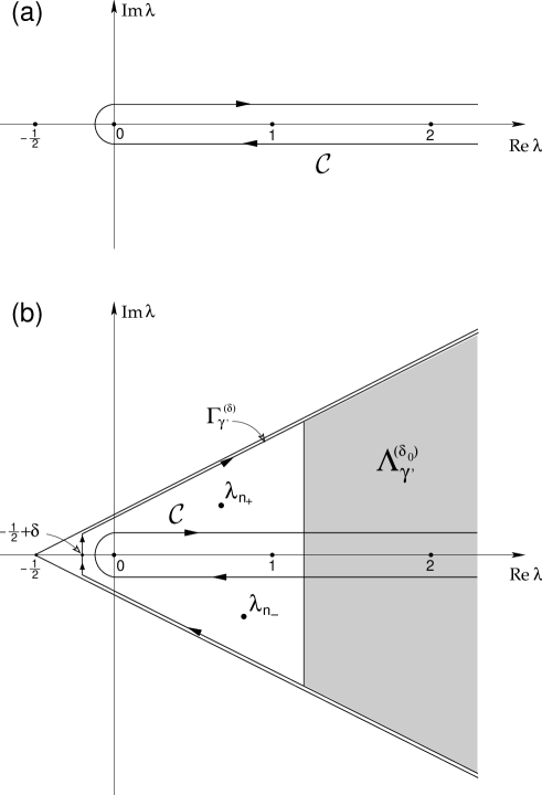
Figure 2: (a): the integration path $\mathcal{C}$ in formula (5.1). (b): the integration path $\Gamma=\Gamma_{\gamma^{\prime}}^{(\delta)}$ in formulae (5.3) and (5.4). The grey sector $\Lambda^{(\delta_{0})}_{\gamma^{\prime}}$ represents a region without poles for the function $a(\lambda,k;g)$. Typical poles, namely $\lambda_{n_{+}}$ and $\lambda_{n_{-}}$, are indicated in the first and fourth quadrants, respectively.

5.2 Analysis of resonances and antiresonances as contributions of poles in the $\boldsymbol{\lambda}$–plane.

We shall now apply the previous Watson–type representation (5.4) of the total scattering amplitude $F(k,\cos\theta;g)$ to the computation of the set of partial waves $a_{\ell}(k;g)$, $(\ell=0,1,\ldots)$, which are defined by the standard inversion formula of expansion (3.159):

$$a_{\ell}(k;g)=\frac{1}{2}\int_{-1}^{+1}F(k,\cos\theta;g)\,P_{\ell}(\cos\theta)\,\mathrm{d}(\cos\theta).$$ (5.8)

For this purpose, we shall use the basic projection formula (see [32, Vol. 1, p. 170, Eq. (7)]):

$$\frac{1}{2}\int_{-1}^{1}P_{\ell}(\cos\theta)\,P_{\lambda}(-\cos\theta)\,\mathrm{d}(\cos\theta)=\frac{\sin\pi\lambda}{\pi(\lambda-\ell)(\lambda+\ell+1)}.$$ (5.9)

By plugging the expression (5.4) of $F$ in (5.8) and applying (5.9) to the various terms, one obtains:

$$a_{\ell}(k;g)=\frac{\mathrm{i}}{2\pi}\int_{\Gamma}\frac{(2\lambda+1)\,a(\lambda,k;g)}{(\lambda-\ell)(\lambda+\ell+1)}\,\mathrm{d}\lambda-\sum_{n=1}^{N}\frac{\rho_{n}(k;g)}{(\lambda_{n}(k;g)-\ell)(\lambda_{n}(k;g)+\ell+1)}.$$ (5.10)

In the r.h.s. of the latter, we distinguish the so–called “background integral” over $\Gamma$ (which is always convergent in view of the exponential decrease property (4.59)) from the individual contributions of the poles $\lambda=\lambda_{n}(k;g)$ of $a(\lambda,k;g)$.

We will show that under certain simple assumptions these poles can be seen to induce properties of the partial waves $a_{\ell}(k;g)$, which are characteristic of resonances and antiresonances; these properties are:

(i) the rapid variation in the momentum variable $k$ (or the energy $E=k^{2}$), including the passage through $\frac{\pi}{2}$ ($\mathrm{mod.}\pi$), of the phase–shift function $k\mapsto\delta_{\ell}(k;g)$, which satisfies (in view of (3.133)):

$$a_{\ell}(k;g)=\frac{e^{\mathrm{i}\delta_{\ell}(k;g)}\sin\delta_{\ell}(k;g)}{k}\qquad(k\in\mathbb{R}^{+}),$$ (5.11)

and therefore:

$$\delta_{\ell}(k;g)=\mathop{\mathrm{Arg}}a_{\ell}(k;g)\ \mathrm{mod.}\ \pi.$$ (5.12)

Resonances (resp., antiresonances) are characterized by the upward (resp., downward) passage of the phase–shift through $\pm\frac{\pi}{2}$ at a certain value $k=k_{\mathrm{r}}$ (resp., $k=k_{\mathrm{ar}}$) at which (in view of (5.11)) $a_{\ell}(k;g)=\mathrm{i}/k$.

In the basic literature on the subject (see, e.g., [1, Chapter 2, Subsection 2.11 (c)]), the quantity $2\,{\partial\delta_{\ell}/\partial E}$ ($=\frac{1}{k}\times{\partial\delta_{\ell}/\partial k}$), whose positive or negative sign plays a role in the previous description of resonances or antiresonances, has been interpreted in terms of the time–delay or time–advance that the incident wave–packet undergoes in the scattering process, in a sense which has been introduced by Eisenbud.

(ii) The production of a “bump” around $k=k_{\mathrm{r}}$ or $k_{\mathrm{ar}}$ in the plot of the function $k\mapsto|a_{\ell}(k;g)|$ and therefore of the cross–section $\sigma_{\mathrm{c}}(k;g)$, since one can write

$$\sigma_{\mathrm{c}}(k;g)=4\pi\,(2\ell+1)\,|a_{\ell}(k;g)|^{2}+4\pi\sum_{\ell^{\prime}\neq\ell}(2\ell^{\prime}+1)\,|a_{\ell^{\prime}}(k;g)|^{2},$$ (5.13)

the sum at the r.h.s. of the latter being subdominant near $k=k_{\mathrm{r}}$ or $k_{\mathrm{ar}}$.

Assumptions. We shall concentrate on the function $a_{\ell}(k;g)$ for given fixed values of $\ell$ and $g$, and assume that among the various poles $\lambda=\lambda_{n}(k;g)$ of the meromorphic function $a(\lambda,k;g)$ which contribute to the sum on the r.h.s. of Eq. (5.10), there exists a distinguished pole, denoted simply by $\lambda(k;g)$, with the corresponding residue $\rho(k;g)=|\rho(k;g)|e^{\mathrm{i}\varphi(k;g)}$. We assume that the corresponding analytic function $k\mapsto\lambda(k;g)$ satisfies the following properties:

There exists a finite interval $I=\{k\,:\,0<k_{\min}<k<k_{\max}\}$ such that for $k\in I$:

• The function $k\mapsto\alpha(k;g)=\mathop{\mathrm{Re}}\lambda(k;g)$ is an increasing function such that for a certain value $k=k_{\ell}\in I$ one has: $\alpha(k_{\ell};g)=\ell$.
  

• The function $k\mapsto\beta(k;g)=\mathop{\mathrm{Im}}\lambda(k;g)$ is such that $0<|\beta(k;g)|\ll 1$ and $|{(\partial\beta/\partial k)}(k;g)|\ll{(\partial\alpha/\partial k)}(k;g)$.
  

• “One–pole dominance”: $|a_{\ell}(k;g)-\widehat{a}_{\ell}(k;g)|\ll 1$, where we have put:

  $$\widehat{a}_{\ell}(k;g)=\frac{-\rho(k;g)}{[\lambda(k;g)-\ell]\,[\lambda(k;g)+\ell+1]}.$$ (5.14)

We shall then consider that the unitarity relation

$$k\,|a_{\ell}(k;g)|^{2}-\mathop{\mathrm{Im}}a_{\ell}(k;g)=0,$$ (5.15)

(implemented by the parametrization (5.11)) is approximately satisfied by this one–pole dominant contribution $\widehat{a}_{\ell}(k;g)$ itself. Applying this approximation yields the following relation between the modulus and the argument $\varphi$ of the residue $\rho$:

$$|\rho|=\frac{1}{k}\left\{(\sin\varphi)\,\left[-(\alpha-\ell)(\alpha+\ell+1)+\beta^{2}\right]+(\cos\varphi)\,\beta\,(2\alpha+1)\right\},$$ (5.16)

which, in particular, yields for $k=k_{\ell}$ (in view of (a)):

$$|\rho(k_{\ell};g)|=\frac{(\cos\varphi)\,\beta(k_{\ell})\,(2\ell+1)}{k_{\ell}}+O\left([\beta(k_{\ell})]^{2}\right),$$ (5.17)

and therefore, in view of assumption (c):

$$|a_{\ell}(k_{\ell};g)|\,\approx\,|\widehat{a}_{\ell}(k_{\ell};g)|\approx\frac{|\cos\varphi(k_{\ell};g)|}{k_{\ell}}.$$ (5.18)

5.2.1 Variation of the phase–shift near $\boldsymbol{k=k_{\ell}}$.

In view of assumption (c) and of (5.12), and by taking the arguments of both sides of Eq. (5.14), one then obtain:

$$\delta_{\ell}(k;g)\approx\varphi(k;g)\pm\pi-\mathop{\mathrm{Arg}}(\lambda(k;g)-\ell)-\mathop{\mathrm{Arg}}(\lambda(k;g)+\ell+1).$$ (5.19)

A simple geometrical analysis, making an essential use of assumption (a), shows that:

(1)  If $\beta(k;g)$ is positive, the function $k\mapsto\delta_{\ell}(k;g)$ admits an upward variation from a value of the form $(\varphi(k;g)+\varepsilon)$ to $(\varphi(k;g)+\pi-\varepsilon)$ for $k$ varying on a short interval $[k_{-},k_{+}]$ centered at $k_{\ell}$. (In view of the assumption $\beta(k;g)\ll 1$, the size of this interval is such that: $\ell-1<\alpha(k_{-})<\ell<\alpha(k_{+})<\ell+1$, provided $\varepsilon$ is chosen sufficiently small). We thus conclude that in a “generic way” (i.e., except if $\varphi(k;g)=\pm\frac{\pi}{2}$), the interval $[k_{-},k_{+}]$ will contain a value $k=k_{\mathrm{r}}$ at which $\delta_{\ell}(k_{\mathrm{r}};g)=\pm\frac{\pi}{2}$, which therefore exhibits the typical behaviour of a resonance at $k=k_{\mathrm{r}}$.

(2)  Similarly, if $\beta(k;g)$ is negative, the function $k\to\delta_{\ell}(k;g)$ admits a downward variation from $(\varphi(k;g)-\varepsilon)$ to $(\varphi(k;g)-\pi+\varepsilon)$ for $k$ varying on a short interval $[k_{-},k_{+}]$ centered at $k_{\ell}$. The latter also contains (in a generic way) a value $k=k_{\mathrm{ar}}$ at which $\delta_{\ell}(k_{\mathrm{ar}};g)=\pm\frac{\pi}{2}$, which then exhibits the typical behaviour of an antiresonance at $k=k_{\mathrm{ar}}$.

Bump for the cross–section near $\boldsymbol{k=k_{\ell}}$.  In both cases (1) and (2) of the previous analysis, one has, in view of (5.11):

$$|a_{\ell}(k_{\mathrm{r},\mathrm{ar}})|=\frac{1}{\ k_{\mathrm{r},\mathrm{ar}}},$$ (5.20)

(where $k_{\mathrm{r},\mathrm{ar}}=k_{\mathrm{r}}$ or $k_{\mathrm{ar}}$), and therefore the plot of the partial wave $a_{\ell}(k;g)$ exhibits a bump around $k=k_{\mathrm{r},\mathrm{ar}}$ which is tangent to the upper limiting curve $|a_{\ell}^{\max}(k;g)|={1/k}$. One can also notice the difference between (5.20) and the value (5.18) of $|\widehat{a}_{\ell}(k_{\ell};g)|$, which (if $|\cos\varphi(k_{\ell};g)|\neq 1$) expresses the rapid variation of the phase–shift between $k_{\ell}$ and $k_{\mathrm{r},\mathrm{ar}}$. Finally, in view of (5.13), the plot of the cross–section $\sigma_{\mathrm{c}}(k;g)$ will also present a bump in an interval of the momentum variable containing the values $k_{\ell}$ and $k_{\mathrm{r},\mathrm{ar}}$.

5.3 Connection between descriptions of phenomena in the $\boldsymbol{\lambda}$–plane and in the $\boldsymbol{k}$–plane.

The description of resonances and antiresonances of a given partial wave $a_{\ell}(k;g)$, which has been given above, appeared to be completely symmetric. In both cases indeed, it was based on the assumption of a dominant one–pole approximation of the partial scattering function $a(\lambda,k;g)$ in the complex $\lambda$–plane, such that the dominant pole $\lambda=\lambda(k;g)$ be located at a very small distance $|\beta(k;g)|$ from the real axis; the two cases are distinguished from each other by the sign of the function $k\mapsto\beta(k;g)$.

We are now going to show that, in spite of the previous apparent symmetry, these two cases necessarily correspond to completely different types of analyticity properties of the dominant function $k\mapsto\widehat{a}_{\ell}(k;g)$ in the complex $k$–plane.

(1) The case of resonances.

In the r.h.s. of (5.14), it is the factor $\lambda(k;g)-\ell=\alpha(k;g)-\ell+{\mathrm{i}}\beta(k;g)$ at the denominator which is responsible for the rapid variation of $\delta_{\ell}(k;g)$ near $k=k_{\ell}$, and whose vanishing in the complex $k$–plane must be analysed. Since the function $(k\ \mathrm{real})\mapsto\lambda(k;g)$ is holomorphic in a small complex neighbourhood $\mathcal{V}$ of $k\ell$, one can postulate the validity (in $\mathcal{V}$) of the following first–order Taylor approximation $\lambda(k;g)\approx\ell+\mathrm{i}\beta(k_{\ell};g)+\frac{\partial\lambda}{\partial k}(k_{\ell};g)\ (k-k_{\ell})$, which therefore yields:

$$\lambda(k;g)-\ell\approx\frac{\partial\lambda}{\partial k}(k_{\ell};g)\ [(k-k_{\ell})+\mathrm{i}\gamma],$$ (5.21)

where we have put:

$$\gamma=\frac{\beta(k_{\ell};g)}{\frac{\partial\lambda}{\partial k}(k_{\ell};g)}.$$ (5.22)

Since it was supposed that $\left|\frac{\partial\beta}{\partial k}\right|\ll\frac{\partial\alpha}{\partial k}$, we can say that $\frac{\partial\lambda}{\partial k}(k_{\ell};g)\approx\frac{\partial\alpha}{\partial k}$, which is real and positive, and (in view of (5.22)) this positivity property is also true for $\gamma$. In view of (5.21), the expression (5.14) of $\widehat{a}_{\ell}(k;g)$ therefore factorizes a pole located at $k=k_{\ell}-\mathrm{i}\gamma$, and $\gamma$ can thus be related to the standard width parameter of the Breit–Wigner one–pole approximation.

The shape of the bump for the cross–section:

If one first considers the case when the residue $\rho(k;g)$ is real (for $k$ real), so that, in view of (5.16): $\rho=\frac{\beta(2\alpha+1)}{k}>0$, we can see that the expression (5.14) of $\widehat{a}_{\ell}(k;g)$ can be approximated by

$$\frac{-\beta}{k\,(\alpha-\ell+\mathrm{i}\beta)}\approx\frac{-\gamma}{k\,(k-k_{\ell}+\mathrm{i}\gamma)}.$$ (5.23)

This approximation, which is valid for $k$ varying in a suitable interval centered at $k_{\ell}$, gives the standard Lorentzian contribution to the cross–section, namely:

$$\widehat{\sigma}_{\ell}(k;g)\approx\frac{4\pi\gamma^{2}}{k^{2}[(k-k_{\ell})^{2}+\gamma^{2}]}.$$ (5.24)

In the general case, the residue is complex and satisfies Eq. (5.16). Then, by taking Eqs. (5.21) and (5.22) into account, expression (5.14) now yields a contribution to the cross–section which is of the following form:

$$\widehat{\sigma}_{\ell}(k;g)\approx\frac{4\pi[\sin\varphi(k;g)\ (k-k_{\ell})-\gamma\,\cos\varphi(k;g)]^{2}}{k^{2}\,[(k-k_{\ell})^{2}+\gamma^{2}]}.$$ (5.25)

This asymmetric contribution corresponds to the generalized form of a Breit–Wigner one–pole model, when the unitary partial wave $S_{\ell}(k)$ includes an additional phase function $\varphi(k)$, namely:

$$S_{\ell}(k)=e^{2\mathrm{i}\varphi(k)}\ \frac{k-k_{0}-\mathrm{i}\gamma}{k-k_{0}+\mathrm{i}\gamma}.$$ (5.26)

(2) The case of antiresonances.

In view of the apparent symmetric treatment of resonances and antiresonances that we have given above, one would be tempted to apply again the previous Taylor expansion argument to the analysis of the factor $[\lambda(k;g)-\ell]$ when $\beta(k;g)$ is negative. However, the analog of formula (5.21) would exhibit a pole in the upper half–plane at $k=k_{\ell}-\mathrm{i}\gamma$, with $\gamma<0$, corresponding to the real value $\lambda=\ell$. But such a result is contradictory with the constraint imposed by the Wronskian Lemma (see, after Lemma 4.10, the paragraph (a) in “Application: regions of $(\lambda,k)$–space free of singularities”). This impossibility of having singular pairs $(\lambda,k)$ at $\lambda$ real and $\mathop{\mathrm{Re}}k>0$, $\mathop{\mathrm{Im}}k>0$, which was known to hold in general for local potentials, has indeed be extended here to the large classes $\mathcal{N}^{\,\gamma}_{{w^{(\varepsilon)}\!,\alpha}}$ of nonlocal potentials.

In order to have a full account of antiresonances associated with dominant poles of $a(\lambda,k;g)$ that may be produced by the theory of nonlocal potentials, one is thus faced to imagine the following type of mathematical model: construct a holomorphic function $k\mapsto\lambda(k;g)$ satisfying the three previous assumptions (a), (b), and (c) with $\beta(k;g)=\mathop{\mathrm{Im}}\lambda(k;g)<0$ for $k\in[k_{-},k_{+}]$, and such that, in addition, $\mathop{\mathrm{Im}}\lambda(k;g)$ remains strictly negative when $k$ varies in the upper half–plane.

As a tutorial model, one can propose the following function:

$$\lambda(k)=\ell+\mathrm{i}\,\frac{\beta_{0}}{2}\left[1+\frac{e^{c(k-k_{\ell})^{2}}}{1-\mathrm{i}(k-k_{\ell})}\right]\qquad(\beta_{0}<0;\ \ \ell={\rm fixed}\ \ {\rm integer}).$$ (5.27)

In fact, one can check that if $\mathop{\mathrm{Re}}k$ varies in some positive interval $I$ depending on $c$ ($c>0$) and centered at $k_{\ell}$, then:

• for real $k$, ${\partial\alpha/\partial k}$ is a positive function, and $\beta(k)$ remains of the order of $\beta_{0}$;
  

• for all $k=\mathop{\mathrm{Re}}k+\mathrm{i}\gamma$, with $\gamma>0$, one has $\mathop{\mathrm{Im}}\lambda(k)<0$.

Then, if we choose as a dominant–pole contribution the function $\widehat{a}_{\ell}(k)$ associated with $\lambda(k)$ by formula (5.14), it satisfies the characteristic phase–shift properties of an antiresonance near $k=k_{\ell}$; thus, according to the previous general analysis, its corresponding contribution to the cross–section produces a bump near $k=k_{\ell}$, but the mathematical description of this bump involves a Gaussian–type behaviour instead of the familiar Lorentzian behaviour, as it is produced by the Breit–Wigner–type pole in the case of a resonance.

Of course, the value of the previous example is limited to the description of local phenomena related to a given partial wave amplitude $a_{\ell}(k)$. As a matter of fact, one should expect that, in the same way as a “Regge trajectory” $\lambda=\lambda(k)$ with $\beta>0$ is able to describe a sequence of resonances, whose angular momentum $\ell$ increases with $k$, a similar “image–trajectory” $\lambda=\lambda(k)$ with $\beta<0$ might correspondingly describe a sequence of antiresonances, whose angular momentum $\ell$ would also increase with $k$. The expectation of an alternating sequence of resonances and antiresonances associated with increasing values of $\ell$ and $k$ seems indeed suggested by the phenomenological study of various nuclear scattering processes (see [10] and [11]). A strong hope exists that the theory of nonlocal potentials (in particular within the classes that have been studied in the present paper) may be able to produce such type of coupled trajectories belonging respectively to the first and to the fourth quadrant in the $\lambda$–plane, a possibility which was forbidden by the usual theory of local potentials.

Appendix A Bounds on the “angular–momentum Green function”

A.I Discrete angular momentum analysis

We shall use the partial wave expansion of the (free–Hamiltonian) Green function:

$$g(\cos\theta,k;R,R^{\prime}) \doteq\frac{1}{4\pi}\,\frac{e^{\mathrm{i}k|\boldsymbol{R}-\boldsymbol{R}^{\prime}|}}{|\boldsymbol{R}-\boldsymbol{R}^{\prime}|}=\frac{1}{4\pi}\,\frac{e^{\mathrm{i}k(R^{2}+{R^{\prime}}^{2}-2RR^{\prime}\cos\theta)^{1/2}}}{(R^{2}+{R^{\prime}}^{2}-2RR^{\prime}\cos\theta)^{1/2}},$$ (A.1)

namely:

$$g(\cos\theta,k;R,R^{\prime}) =-\sum_{\ell=0}^{\infty}\ (2\ell+1)\ \frac{G_{\ell}(k;R,R^{\prime})}{4\pi RR^{\prime}}\ P_{\ell}(\cos\theta),$$ (A.2)

in which the set of coefficients $G_{\ell}(k;R,R^{\prime})$, called “angular–momentum Green function” are given by:

$$G_{\ell}(k;R,R^{\prime})=-2\pi RR^{\prime}\int_{-1}^{+1}g(\cos\theta,k;R,R^{\prime})\ P_{\ell}(\cos\theta)\,\mathrm{d}\cos\theta.$$ (A.3)

Relations (3.10e): i.e., $G_{\ell}(k;R,R^{\prime})=-\mathrm{i}kRR^{\prime}j_{\ell}[k\min(R,R^{\prime})]\ h_{\ell}^{(1)}[k\max(R,R^{\prime})]$, (implied by the fact that $G_{\ell}$ satisfies Bessel equations with appropriate boundary conditions separately with respect to $R$ and $R^{\prime}$) will not be used here, since we shall obtain relevant bounds on $G_{\ell}$ by direct use of formula (A.3).

In formula (A.3), $k$ may be real or complex, namely the functions $G_{\ell}$ are defined for all $R>0$, $R^{\prime}>0$ as entire functions of $k$, and one has:

$$4\pi\,|g(\cos\theta,k;R,R^{\prime})|=\frac{e^{-\mathop{\mathrm{Im}}k\ [(R-R^{\prime})^{2}+2RR^{\prime}(1-\cos\theta)]^{\frac{1}{2}}}}{[(R-R^{\prime})^{2}+2RR^{\prime}(1-\cos\theta)]^{\frac{1}{2}}}.$$ (A.4)

For $\mathop{\mathrm{Im}}k\geqslant 0$, the latter is uniformly bounded by $[2RR^{\prime}(1-\cos\theta)]^{-\frac{1}{2}}$, while for $\mathop{\mathrm{Im}}k<0$ it is uniformly bounded by $\frac{e^{|\mathop{\mathrm{Im}}k|\ (R+R^{\prime})}}{[2RR^{\prime}(1-\cos\theta)]^{\frac{1}{2}}}$. From (A.3) one thus obtains the following global majorization:

$$\begin{split}&|G_{\ell}(k;R,R^{\prime})|\leqslant\frac{1}{2}(RR^{\prime})^{\frac{1}{2}}\max\left(1,e^{-\mathop{\mathrm{Im}}k(R+R^{\prime})}\right)\int_{-1}^{+1}\frac{|P_{\ell}(t)|}{\sqrt{2(1-t)}}\,\mathrm{d}t\\ &\quad\leqslant\frac{1}{2}\max\left(1,e^{-\mathop{\mathrm{Im}}k(R+R^{\prime})}\right)\left(\frac{\pi RR^{\prime}}{2\ell+1}\right)^{\frac{1}{2}}.\end{split}$$ (A.5)

For writing the rightmost inequality of (A.5), we have used the Martin inequality (see [40]) $|P_{\ell}(\cos\theta)|<\min\left(1,2\,[\ell\pi\sin\theta]^{-1/2}\right)$. (Note that for $k$ real, bound (A.5) itself lies in [40]).

We shall now derive an alternative bound on $G_{\ell}$, which exhibits a decrease property with respect to $|k|$ ($k\in\mathbb{C}$). Let us rewrite Eq. (A.3) as follows, by introducing the change of integration variable $u=[R^{2}+{R^{\prime}}^{2}-2RR^{\prime}\cos\theta]^{\frac{1}{2}}$, i.e., $\cos\theta(u)=\frac{R^{2}+{R^{\prime}}^{2}-u^{2}}{2RR^{\prime}}$:

$$G_{\ell}(k;R,R^{\prime})=\frac{1}{2}\int_{|R-R^{\prime}|}^{R+R^{\prime}}e^{\mathrm{i}ku}\ P_{\ell}(\cos\theta(u))\,\mathrm{d}u.$$ (A.6)

We now have (by using integration by parts):

$$\begin{split}&\mathrm{i}kG_{\ell}(k;R,R^{\prime})=\frac{1}{2}\int_{|R-R^{\prime}|}^{R+R^{\prime}}\frac{\mathrm{d}}{\mathrm{d}u}[e^{\mathrm{i}ku}]\ P_{\ell}(\cos\theta(u))\,\mathrm{d}u\\ &\quad=\frac{1}{2RR^{\prime}}\int_{|R-R^{\prime}|}^{R+R^{\prime}}e^{\mathrm{i}ku}\ P^{\prime}_{\ell}(\cos\theta(u))\,u\,\mathrm{d}u\,+\frac{1}{2}\left[e^{\mathrm{i}k(R+R^{\prime})}-(-1)^{\ell}e^{\mathrm{i}k|R-R^{\prime}|}\right],\end{split}$$ (A.7)

(where we have used the fact that $P_{\ell}(1)=1$, $P_{\ell}(-1)=(-1)^{\ell}$).

From the integral representation $P_{\ell}(\cos\theta)=\frac{1}{\pi}\int_{0}^{\pi}(\cos\theta+\mathrm{i}\sin\theta\cos\alpha)^{\ell}\,\mathrm{d}\alpha$, one readily obtains the following bound

$$|P^{\prime}_{\ell}(\cos\theta)|\leqslant\frac{\ell}{|\sin\theta|}.$$ (A.8)

The latter allows one to give a majorization for the r.h.s. of Eq. (A.7), which yields:

$$|k|\,|G_{\ell}(k;R,R^{\prime})|\leqslant\,\max\left(1,e^{-\mathop{\mathrm{Im}}k(R+R^{\prime})}\right)\left[1+\frac{\ell}{2}\int_{|R-R^{\prime}|}^{R+R^{\prime}}\frac{u\,\mathrm{d}u}{RR^{\prime}\,|\sin\theta(u)|}\right].$$ (A.9)

Since $2RR^{\prime}\sin\theta(u)=[(R+R^{\prime}+u)(R+R^{\prime}-u)(u+R-R^{\prime})(u+R^{\prime}-R)]^{\frac{1}{2}}$, one then gets the following majorization:

$$\frac{\ell}{2}\int_{|R-R^{\prime}|}^{R+R^{\prime}}\frac{u\,\mathrm{d}u}{RR^{\prime}\,|\sin\theta|}\leqslant\ell\int_{|R-R^{\prime}|}^{R+R^{\prime}}\frac{\mathrm{d}u}{(R+R^{\prime}-u)^{\frac{1}{2}}\,(u-|R-R^{\prime}|)^{\frac{1}{2}}}=\ell\pi,$$ (A.10)

and therefore, from (A.9):

$$|G_{\ell}(k;R,R^{\prime})|\leqslant\,\max\left(1,e^{-\mathop{\mathrm{Im}}k(R+R^{\prime})}\right)\left(\frac{1+\ell\pi}{|k|}\right).$$ (A.11)

As a result of (A.5) and (A.11), we can thus write the following global uniform bound, which exhibits decrease properties with respect to both variables $\ell$ and $|k|$ when they go to infinity:

$$|G_{\ell}(k;R,R^{\prime})|\leqslant\max\left(1,e^{-\mathop{\mathrm{Im}}k(R+R^{\prime})}\right)[1+R]^{\frac{1}{2}}\,[1+R^{\prime}]^{\frac{1}{2}}\min\left(\frac{\ell\pi+1}{|k|},\frac{1}{2}\sqrt{\frac{\pi}{2\ell+1}}\,\right).$$ (A.12)

A.II Complex angular momentum analysis

We shall now introduce a function $G(\lambda,k;R,R^{\prime})$, called the complex–angular–momentum Green function, defined for all complex $\lambda$ in the half–plane ${\mathbb{C}^{+}_{-\frac{1}{2}}}=\left\{\lambda\,:\,\mathop{\mathrm{Re}}\lambda>-\frac{1}{2}\right\}$, such that for all positive integers $\ell$, one has: $G_{\ell}(k;R,R^{\prime})=G(\ell,k;R,R^{\prime})$. For every $R$, $R^{\prime}$ ($R>0$, $R^{\prime}>0$), the function $G$ will be uniquely defined as a holomorphic function of $(\lambda,k)$ in the product $\mathbb{C}^{+}_{-\frac{1}{2}}\times\widehat{\mathbb{C}}$, where $\widehat{\mathbb{C}}$ denotes the universal covering of $\mathbb{C}\setminus\{0\}$. The uniqueness of this interpolation of $G_{\ell}$ will be ensured by the fact that for $k=\mathrm{i}\kappa$, $\kappa>0$, $G(\lambda,\mathrm{i}\kappa;R,R^{\prime})$ is a Carlsonian interpolation, which will thus allow us to specify the “basic” first–sheet ${\mathbb{C}^{\mathop{(\mathrm{cut})}}}\doteq\mathbb{C}\setminus(-\infty,0]$ of $G$. Our purpose now is the derivation of uniform bounds for $|G(\lambda,k;R,R^{\prime})|$ in $\left\{(\lambda,k)\in\mathbb{C}^{+}_{-\frac{1}{2}}\times\mathbb{C}^{\mathop{(\mathrm{cut})}}\right\}$.

(1) Analysis for $\boldsymbol{k=\mathrm{i}\kappa}$, $\boldsymbol{\kappa>0}$.

Let $z_{0}\equiv z_{0}(R,R^{\prime})=\frac{1}{2}\left(\frac{R}{R^{\prime}}+\frac{R^{\prime}}{R}\right)$. For $k=\mathrm{i}\kappa$, $\kappa>0$, the Green function $g$ (see (A.1)) can be conveniently rewritten as follows in terms of the complex variable $z=\cos\theta$:

$$g(z,\mathrm{i}\kappa;R,R^{\prime})=\frac{1}{4\pi}\,\frac{e^{-\kappa(2RR^{\prime})^{\frac{1}{2}}(z_{0}-z)^{\frac{1}{2}}}}{(2RR^{\prime})^{\frac{1}{2}}\,(z_{0}-z)^{\frac{1}{2}}}.$$ (A.13)

Since the function $u(R,R^{\prime};z)\doteq(2RR^{\prime})^{\frac{1}{2}}(z_{0}-z)^{\frac{1}{2}}$ (specified as being positive for $z$ real, $z<z_{0}$) is such that $\mathop{\mathrm{Re}}u(R,R^{\prime};z)\geqslant 0$ for z varying in the (closed) cut–plane ${\mathbb{C}^{\mathop{(\mathrm{cut})}}_{z_{0}}}\doteq\mathbb{C}\setminus[z_{0},+\infty[$, the following uniform bound holds:

$$\mathrm{For}\ z\in\mathbb{C}^{\mathop{(\mathrm{cut})}}_{z_{0}},\qquad|g(z,\mathrm{i}\kappa;R,R^{\prime})|\leqslant\frac{1}{4\pi}\frac{1}{(2RR^{\prime})^{\frac{1}{2}}\,|z_{0}-z|^{\frac{1}{2}}}.$$ (A.14)

It follows that, as a holomorphic function of $z$, $g(z,\mathrm{i}\kappa;R,R^{\prime})$ satisfies the conditions of the Froissart–Gribov theorem (or Laplace–transformation on the one–sheeted hyperboloid in the sense of [36]). Therefore, there exists a function $G(\lambda,\mathrm{i}\kappa;R,R^{\prime})$, holomorphic in the half–plane $\left\{\lambda\in{\mathbb{C}^{+}_{-\frac{1}{2}}}\right\}$ such that for all integers $\ell$ ($\ell\geqslant 0$), one has $G(\ell,\mathrm{i}\kappa;R,R^{\prime})=G_{\ell}(\mathrm{i}\kappa;R,R^{\prime})$. Moreover, this function $G$ is given by the following integral in terms of the discontinuity $\Delta g$ of $g$ across the cut $z\in[z_{0},+\infty[$, namely $\Delta g(z,\mathrm{i}\kappa;R,R^{\prime})=\frac{1}{4\pi}\frac{\cos\left[\kappa(2RR^{\prime})^{\frac{1}{2}}(z-z_{0})^{\frac{1}{2}}\right]}{(2RR^{\prime})^{\frac{1}{2}}(z-z_{0})^{\frac{1}{2}}}$:

$$G(\lambda,\mathrm{i}\kappa;R,R^{\prime})=-\frac{RR^{\prime}}{2}\int_{z_{0}(R,R^{\prime})}^{+\infty}\frac{\cos\left(\kappa\,(2RR^{\prime})^{\frac{1}{2}}(z-z_{0})^{\frac{1}{2}}\right)}{(2RR^{\prime})^{\frac{1}{2}}(z-z_{0})^{\frac{1}{2}}}\,Q_{\lambda}(z)\,\mathrm{d}z.$$ (A.15)

In this equation, $Q_{\lambda}$ denotes the second–kind Legendre function, and we note that the integral is convergent for all $\lambda$ in ${\mathbb{C}^{+}_{-\frac{1}{2}}}$.

Bounds on $G(\lambda,i\kappa;R,R^{\prime})$:

(a)  In view of (A.15), we have:

$$|G(\lambda,\mathrm{i}\kappa;R,R^{\prime})|\leqslant\frac{(RR^{\prime})^{\frac{1}{2}}}{2\sqrt{2}}\int_{z_{0}(R,R^{\prime})}^{+\infty}\frac{|Q_{\lambda}(z)|}{[z-z_{0}(R,R^{\prime})]^{\frac{1}{2}}}\,\mathrm{d}z.$$ (A.16)

Then, by using the following integral representation of $Q_{\lambda}$ (see, e.g., [36, formula (III–11)]):

$$Q_{\lambda}(z)=\frac{1}{\pi}\int_{v\doteq\cosh^{-1}\!z}^{+\infty}e^{-(\lambda+\frac{1}{2})w}\ [2(\cosh w-\cosh v)]^{-\frac{1}{2}}\,\mathrm{d}w,$$ (A.17)

and the relation $\cosh^{-1}\!z_{0}(R,R^{\prime})=\left|\ln\frac{R}{R^{\prime}}\right|$, we obtain:

$$\int_{z_{0}(R,R^{\prime})}^{+\infty}\frac{|Q_{\lambda}(z)|}{[z-z_{0}(R,R^{\prime})]^{\frac{1}{2}}}\,\mathrm{d}z\leqslant\frac{1}{\pi}\int_{\left|\ln\frac{R}{R^{\prime}}\right|}^{+\infty}e^{-(\mathop{\mathrm{Re}}\lambda+\frac{1}{2})w}\,\mathrm{d}w\int_{z_{0}(R,R^{\prime})}^{\zeta\doteq\cosh w}\frac{\mathrm{d}z}{\{2(\zeta-z)\,[z-z_{0}(R,R^{\prime})]\}^{\frac{1}{2}}}.$$ (A.18)

But, since the subintegral in the r.h.s of (A.18) is equal to the constant $\frac{\pi}{\sqrt{2}}$, we obtain, in view of (A.16) and (A.17):

$$|G(\lambda,\mathrm{i}\kappa;R,R^{\prime})|\leqslant\frac{(RR^{\prime})^{\frac{1}{2}}}{2(2\mathop{\mathrm{Re}}\lambda+1)}\ \left[\min\left(\frac{R}{R^{\prime}},\frac{R^{\prime}}{R}\right)\right]^{(\mathop{\mathrm{Re}}\lambda+\frac{1}{2})}.$$ (A.19)

(b)   We shall now derive an alternative bound on $G$, which exhibits a decrease property with respect to $\kappa$. By making use of the integration variable $\widehat{u}=\widehat{u}(z)=(2RR^{\prime})^{\frac{1}{2}}(z-z_{0})^{\frac{1}{2}}$ and of the inverse mapping $z=z(\widehat{u})=z_{0}+\frac{\widehat{u}^{2}}{2RR^{\prime}}$, we rewrite Eq. (A.15) as follows:

$$G(\lambda,\mathrm{i}\kappa;R,R^{\prime})=-\frac{1}{2}\int_{0}^{+\infty}\cos\kappa\widehat{u}\ Q_{\lambda}(z(\widehat{u}))\,\mathrm{d}\widehat{u}.$$ (A.20)

We then have:

$$\kappa\,G(\lambda,\mathrm{i}\kappa;R,R^{\prime})=-\frac{1}{2}\int_{0}^{+\infty}\frac{\mathrm{d}}{\mathrm{d}\widehat{u}}[\sin\kappa\widehat{u}]\ Q_{\lambda}(z(\widehat{u}))\,\mathrm{d}\widehat{u}=\frac{1}{2}\int_{0}^{+\infty}\sin\kappa\widehat{u}\ \,Q^{\prime}_{\lambda}(z(\widehat{u}))\ \frac{\widehat{u}}{RR^{\prime}}\,\mathrm{d}\widehat{u}.$$ (A.21)

From (A.17) (and making use of a partial integration procedure) we can deduce the following integral representation for $Q^{\prime}_{\lambda}$:

$$Q^{\prime}_{\lambda}(z)=-\frac{\lambda+\frac{1}{2}}{\pi}\int_{z}^{+\infty}\frac{e^{-(\lambda+\frac{1}{2})w}\ \mathrm{d}\zeta}{[2(\zeta-z)]^{\frac{1}{2}}\,(\zeta^{2}-1)}-\frac{1}{\pi}\int_{z}^{+\infty}\frac{e^{-(\lambda+\frac{1}{2})w}\ \zeta\,\mathrm{d}\zeta}{[2(\zeta-z)]^{\frac{1}{2}}\ (\zeta^{2}-1)^{\frac{3}{2}}},$$ (A.22)

in which $w=\cosh^{-1}\!\zeta$. By taking the latter into account in Eq. (A.21) and inverting the integrations over $z$ and $\zeta$, one obtains:

$$\begin{split}&\kappa\,G(\lambda,\mathrm{i}\kappa;R,R^{\prime})=-\frac{\lambda+\frac{1}{2}}{2\pi}\int_{z_{0}}^{+\infty}\frac{e^{-(\lambda+\frac{1}{2})w}}{\zeta^{2}-1}\,\mathrm{d}\zeta\int_{z_{0}}^{\zeta}\frac{\sin\left(\kappa\,(2RR^{\prime})^{\frac{1}{2}}(z-z_{0})^{\frac{1}{2}}\right)}{[2(\zeta-z)]^{\frac{1}{2}}}\,\mathrm{d}z\\ &\quad-\frac{1}{2\pi}\int_{z_{0}}^{+\infty}\frac{e^{-(\lambda+\frac{1}{2})w}}{(\zeta^{2}-1)^{\frac{3}{2}}}\ \zeta\,\mathrm{d}\zeta\int_{z_{0}}^{\zeta}\frac{\sin\left(\kappa\,(2RR^{\prime})^{\frac{1}{2}}(z-z_{0})^{\frac{1}{2}}\right)}{[2(\zeta-z)]^{\frac{1}{2}}}\,\mathrm{d}z.\end{split}$$ (A.23)

A uniform bound for the first term on the r.h.s. of Eq. (A.23) is obtained by simply majorizing the sine–function by one. In fact, this term is majorized in the whole half–plane $\{\lambda\in{\mathbb{C}^{+}_{-\frac{1}{2}}}\}$ by:

$$\frac{\mathop{\mathrm{Re}}\lambda+\frac{1}{2}}{2\pi}\int_{z_{0}(R,R^{\prime})}^{+\infty}\frac{\{2[\zeta-z_{0}(R,R^{\prime})]\}^{\frac{1}{2}}}{(\zeta^{2}-1)}\,\mathrm{d}\zeta\ \leqslant\ A_{1}\times(2\mathop{\mathrm{Re}}\lambda+1),$$ (A.24)

where $A_{1}$ is a numerical constant (independent of $k$, $R$ and $R^{\prime}$). For obtaining a uniform bound for the second term on the r.h.s. of Eq. (A.23) it is necessary to majorize the sine–function: (a) by one in the range $z\geqslant z_{1}\doteq z_{0}+(2RR^{\prime}\kappa^{2})^{-1}$, and (b) by $\kappa(2RR^{\prime})^{\frac{1}{2}}(z-z_{0})^{\frac{1}{2}}$ in the range $z_{0}\leqslant z\leqslant z_{1}$. One is then led to introduce a partition of the integration region into three subregions of the $(z,\zeta)$–plane, namely $R_{1}=\{\zeta\geqslant z_{1},\,z_{0}\leqslant z\leqslant z_{1}\}$, $R_{2}=\{z_{0}\leqslant\zeta\leqslant z_{1},\,z_{0}\leqslant z\leqslant\zeta\}$, and $R_{3}=\{\zeta\geqslant z_{1},\,z_{1}\leqslant z\leqslant\zeta\}$. While the integrals in $R_{1}$ and $R_{2}$ yield uniform majorizations by numerical constants, the integral in $R_{3}$ is majorized by an expression of the form $[a_{1}+a_{2}\max\left(\ln\,(RR^{\prime}\kappa^{2})^{-1},0\right)]$ ($a_{1}$ and $a_{2}$ being numerical constants). By taking all these estimates into account for the r.h.s. of (A.23), one obtains a majorization of the following form in the half–plane $\left\{\lambda\in\mathbb{C}^{+}_{-\frac{1}{2}}\right\}$:

$$\begin{split}&|G(\lambda,\mathrm{i}\kappa;R,R^{\prime})|\leqslant\frac{A_{1}(2\mathop{\mathrm{Re}}\lambda+1)+A_{2}+A_{3}\ln\left(1+(RR^{\prime}\kappa^{2})^{-1}\right)}{\kappa}\\ &\quad\leqslant C\,\frac{2(\mathop{\mathrm{Re}}\lambda+1)+\ln\left(1+\kappa^{-2}\right)}{\kappa}\left[1+\ln\left(1+\frac{1}{R}\right)\right]\left[1+\ln\left(1+\frac{1}{R^{\prime}}\right)\right],\end{split}$$ (A.25)

where $A_{1}$, $A_{2}$, $A_{3}$, and $C$ are suitable numerical constants.

As a result of (A.19) and (A.25), we can thus write the following global uniform bound, which exhibits decrease properties with respect to both variables $\lambda$ and $\kappa$ when they go to infinity:

$$\begin{split}&|G(\lambda,\mathrm{i}\kappa;R,R^{\prime})|\leqslant\left[1+\ln\left(1+\frac{1}{R}\right)+\sqrt{R}\right]\ \left[1+\ln\left(1+\frac{1}{R^{\prime}}\right)+\sqrt{R^{\prime}}\right]\\ &\quad\times\min\left[\frac{1}{2(2\mathop{\mathrm{Re}}\lambda+1)},\ C\,\frac{2(\mathop{\mathrm{Re}}\lambda+1)+\ln\left(1+\kappa^{-2}\right)}{\kappa}\right].\end{split}$$ (A.26)

Bounds on $\frac{\partial}{\partial R}\,G(\lambda,\mathrm{i}\kappa;R,R^{\prime})$:

We shall obtain a relevant expression for this derivative of $G$ by computing the derivative of the double integral on the r.h.s. of Eq. (A.23) with respect to $R$. Using the fact that the successive integrands of the latter in the variables $\zeta$ and $z$ vanish at their common threshold $z_{0}(R,R^{\prime})$, we obtain the following integral representation (in which $w=\cosh^{-1}\!\zeta$):

$$\begin{split}&2\pi\,\frac{\partial}{\partial R}\,G(\lambda,\mathrm{i}\kappa;R,R^{\prime})=\left(\frac{R^{\prime}}{2R}\right)^{\frac{1}{2}}\int_{z_{0}(R,R^{\prime})}^{+\infty}\mathrm{d}\zeta\ e^{-(\lambda+\frac{1}{2})w}\,\left[\frac{\lambda+\frac{1}{2}}{(\zeta^{2}-1)}+\frac{\zeta}{(\zeta^{2}-1)^{\frac{3}{2}}}\right]\\ &\quad\times\!\!\int_{z_{0}(R,R^{\prime})}^{\zeta}\!\!\mathrm{d}z\ \frac{\cos\left(\kappa\,(2RR^{\prime})^{\frac{1}{2}}(z-z_{0})^{\frac{1}{2}}\right)}{[2(\zeta-z)]^{\frac{1}{2}}}\left\{\!\frac{\left[\frac{R}{R^{\prime}}-\frac{R^{\prime}}{R}\right]}{2[z-z_{0}(R,R^{\prime})]^{\frac{1}{2}}}-[z-z_{0}(R,R^{\prime})]^{\frac{1}{2}}\!\right\}\!.\end{split}$$ (A.27)

By proceeding as for the bound (A.19) on $G$, we now deduce the following bound from (A.27):

$$\begin{split}&\left|\frac{\partial}{\partial R}\ G(\lambda,\mathrm{i}\kappa;R,R^{\prime})\right|\\ &\quad\leqslant\frac{1}{4\sqrt{2}}\left(\frac{R^{\prime}}{2R}\right)^{\frac{1}{2}}\left|\frac{R}{R^{\prime}}-\frac{R^{\prime}}{R}\right|\int_{z_{0}(R,R^{\prime})}^{+\infty}e^{-(\mathop{\mathrm{Re}}\lambda+\frac{1}{2})w}\,\left[\frac{|\lambda+\frac{1}{2}|}{(\zeta^{2}-1)}+\frac{\zeta}{(\zeta^{2}-1)^{\frac{3}{2}}}\right]\,\mathrm{d}\zeta\\ &\qquad+\frac{1}{4\sqrt{2}}\left(\frac{R^{\prime}}{2R}\right)^{\frac{1}{2}}\int_{z_{0}(R,R^{\prime})}^{+\infty}\!e^{-(\mathop{\mathrm{Re}}\lambda+\frac{1}{2})w}\left[\frac{|\lambda+\frac{1}{2}|}{(\zeta^{2}-1)}+\frac{\zeta}{(\zeta^{2}-1)^{\frac{3}{2}}}\right][\zeta-z_{0}(R,R^{\prime})]\,\mathrm{d}\zeta.\end{split}$$ (A.28)

By using the inequality $\zeta-z_{0}\leqslant\zeta-1$ one readily obtains that the latter integral in (A.28) is convergent and bounded by a ($\lambda$–dependent) constant in the whole half–plane $\mathbb{C}^{+}_{-\frac{1}{2}}$. By now making the change of variable $u=\sinh w=\sqrt{\zeta^{2}-1}$ in the former integral of (A.28), one also sees that this integral can be majorized (for $\lambda\in\mathbb{C}^{+}_{-\frac{1}{2}}$) by $\left(\left|\lambda+\frac{1}{2}\right|+1\right)\times\int_{\frac{1}{2}\left|\frac{R}{R^{\prime}}-\frac{R^{\prime}}{R}\right|}^{\infty}u^{-2}\,\mathrm{d}u$. As a result, one can replace the inequality (A.28) by a simple majorization of the following form:

$$\left|\frac{\partial}{\partial R}\,G(\lambda,i\kappa;R,R^{\prime})\right|\leqslant c_{1}(\lambda)\times\left(\frac{R^{\prime}}{R}\right)^{\frac{1}{2}},$$ (A.29)

which is valid for all $k=\mathrm{i}\kappa$ ($\kappa>0$) and $\lambda\in\mathbb{C}^{+}_{-\frac{1}{2}}$.

(2) Analytic continuation in $\boldsymbol{k}$.

We start from the definition (A.15) of $G$, in which we insert the integral representation (A.17) of $Q_{\lambda}$ and then invert the integrations over $z$ and $\zeta=\cosh w$. We thus obtain:

$$G(\lambda,\mathrm{i}\kappa;R,R^{\prime})=-\frac{(RR^{\prime})^{\frac{1}{2}}}{2\sqrt{2}\pi}\!\!\int_{z_{0}(R,R^{\prime})}^{+\infty}\!\frac{e^{-(\lambda+\frac{1}{2})w}}{(\zeta^{2}-1)^{\frac{1}{2}}}\,\mathrm{d}\zeta\!\int_{z_{0}}^{\zeta}\!\frac{\cos\left(\!\kappa\,(2RR^{\prime})^{\frac{1}{2}}(z-z_{0})^{\frac{1}{2}}\!\right)}{\{2(\zeta-z)\,[z-z_{0}(R,R^{\prime})]\}^{\frac{1}{2}}}\,\mathrm{d}z.$$ (A.30)

We now wish to define the analytic continuation of this double integral with respect to the complex variable $k$ by putting $k=\mathrm{i}\kappa e^{-\mathrm{i}\phi}$; $\phi$ will be taken in the interval $-\frac{\pi}{2}\leqslant\phi\leqslant\frac{3\pi}{2}$ so that $G$ be defined in the “basic first sheet” ${\mathbb{C}^{\mathop{(\mathrm{cut})}}}$ of the $k$–plane.

(a) For $|\phi|\leqslant\frac{\pi}{2}$, this analytic continuation of $G(\lambda,k;R,R^{\prime})=G(\lambda,\mathrm{i}\kappa e^{-\mathrm{i}\phi};R,R^{\prime})$ is well–defined by shifting in $\mathbb{C}^{2}$ the integration region from its initial situation at $k=\mathrm{i}\kappa$, namely $\Gamma_{0}\doteq\{(\zeta,z)\,:\,z_{0}=z_{0}(R,R^{\prime})\leqslant z\leqslant\zeta<+\infty\}$ to the set $\Gamma_{\phi}\doteq\{(\zeta,z)\,:\,\zeta-z_{0}=|\zeta-z_{0}|e^{2\mathrm{i}\phi},z-z_{0}=|z-z_{0}|e^{2\mathrm{i}\phi};\,z_{0}\leqslant|z|\leqslant|\zeta|<+\infty\}$. The corresponding rotation of angle $\phi$ of $(z-z_{0})^{\frac{1}{2}}$ will then cancel the rotation of angle $-\phi$ of $\kappa$ in the cosine–factor under the integral on the r.h.s. of (A.30), so that this factor can always be bounded by one. It follows that one obtains a majorization for the analytic continuation at $k=\mathrm{i}\kappa e^{-\mathrm{i}\phi}$ of the r.h.s. of (A.30) which involves the same subintegral over $z$ as in (A.18) (equal to the constant $\frac{\pi}{\sqrt{2}}$), namely:

$$|G(\lambda,k;R,R^{\prime})|\leqslant\frac{(RR^{\prime})^{\frac{1}{2}}}{4}\int_{\gamma_{\phi}(z_{0}(R,R^{\prime}))}\left|e^{-(\lambda+\frac{1}{2})(w+\mathrm{i}\varphi)}\right|\,|\mathrm{d}(w+i\varphi)|;$$ (A.31)

in (A.31), $\gamma_{\phi}(z_{0}(R,R^{\prime}))$ is the image of $\widehat{\gamma}_{\phi}\doteq\{\zeta=z_{0}(R,R^{\prime})+\rho e^{2\mathrm{i}\phi},\,\rho\in[0,+\infty)\}$ by the mapping $\zeta\mapsto\widehat{w}\doteq w+\mathrm{i}\varphi=\cosh^{-1}\zeta$. One can check that in the path $\gamma_{\phi}(z_{0}(R,R^{\prime}))$ the variables $|\varphi|$ and $w$ vary respectively in the intervals $|\varphi|\in[0,2\phi]$ and $w\in[w_{0}(R,R^{\prime}),+\infty)$, where $w_{0}(R,R^{\prime})$ is positive and such that:

• if $|\phi|\leqslant\frac{\pi}{4}$, $\cosh w_{0}=z_{0}(R,R^{\prime})=\frac{1}{2}\left(\frac{R}{R^{\prime}}+\frac{R^{\prime}}{R}\right)$, i.e.:

  $$e^{-w_{0}(R,R^{\prime})}=\min\left(\frac{R}{R^{\prime}},\frac{R^{\prime}}{R}\right);$$ (A.32)

• if $\frac{\pi}{4}\leqslant|\phi|\leqslant\frac{\pi}{2}$,  $\cosh^{2}w_{0}(R,R^{\prime})=z_{0}^{2}(R,R^{\prime})\sin^{2}2\phi+\cos^{2}2\phi$, which yields: $\sinh w_{0}(R,R^{\prime})=\frac{1}{2}\left|\frac{R}{R^{\prime}}-\frac{R^{\prime}}{R}\right|\,\sin 2|\phi|$, and thereby:

  $$e^{-w_{0}(R,R^{\prime})}\leqslant(\sin 2|\phi|)^{-1}\,\min\left(\frac{R}{R^{\prime}},\frac{R^{\prime}}{R}\right).$$ (A.33)

Note that in case (i), $\gamma_{\phi}(z_{0}(R,R^{\prime}))$ defines $|\varphi|$ as an increasing function of $w$ in the interval $[w_{0}(R,R^{\prime}),+\infty)$, while in case (ii), $\gamma_{\phi}(z_{0}(R,R^{\prime}))$ is tangent at the line $w=w_{0}(R,R^{\prime})$ at some point $\varphi_{0}$ (with $0\leqslant\varphi_{0}\leqslant\frac{\pi}{2}$).
By taking these geometrical facts into account, one then deduces from (A.31) a majorization of the following form, which is valid for all $k$ in the closed upper half–plane:

$$|G(\lambda,k;R,R^{\prime})|\leqslant\frac{\sqrt{RR^{\prime}}}{4}\int_{\gamma_{\phi}(z_{0})}\!\!\!e^{-(\mathop{\mathrm{Re}}\lambda+\frac{1}{2})w+(\mathop{\mathrm{Im}}\lambda)\varphi}\,|\mathrm{d}(w+\mathrm{i}\varphi)|\leqslant c(\lambda,k)\,\sqrt{RR^{\prime}}\,e^{-(\mathop{\mathrm{Re}}\lambda+\frac{1}{2})w_{0}(R,R^{\prime})},$$ (A.34)

where:

$$c(\lambda,k)=c\,\max\left(e^{2\mathop{\mathrm{Im}}\lambda\,\phi(k)},1\right)\ \left(1+\frac{1}{2\mathop{\mathrm{Re}}\lambda+1}\right).$$ (A.35)

In the latter, $c$ is a numerical constant and $\phi(k)=-\mathop{\mathrm{Arg}}(-\mathrm{i}k)$; more precisely, $k=\mathrm{i}\kappa e^{-\mathrm{i}\phi}$, with $\phi=\phi(k)$ such that $|\phi|\leqslant\frac{\pi}{2}$.

Moreover, by taking Eqs. (A.32) and (A.33) into account, we see that (A.34) implies the following majorization, which is valid globally in the set $\{(\lambda,k)\,:\,\lambda\in\mathbb{C}^{+}_{-\frac{1}{2}};\mathop{\mathrm{Im}}k>0\}$:

$$|G(\lambda,k;R,R^{\prime})|\leqslant c(\lambda,k)\,[\Phi(k)]^{-(\mathop{\mathrm{Re}}\lambda+\frac{1}{2})}\ (RR^{\prime})^{\frac{1}{2}}\left[\min\left(\frac{R}{R^{\prime}},\frac{R^{\prime}}{R}\right)\right]^{\mathop{\mathrm{Re}}\lambda+\frac{1}{2}},$$ (A.36)

in which we have put:

$$\Phi(k) =1\quad\mathrm{if}\quad|\phi(k)|\leqslant\frac{\pi}{4},$$ (A.37)

and

$$\Phi(k) =(\sin 2|\phi(k)|)\quad\mathrm{if}\quad\frac{\pi}{4}\leqslant|\phi(k)|<\frac{\pi}{2}.$$ (A.38)

We also notice that, since $w_{0}(R,R^{\prime})\geqslant 0$, majorization (A.34) also yields for all $k$ in the closed upper half–plane $\mathop{\mathrm{Im}}k\geqslant 0$:

$$|G(\lambda,k;R,R^{\prime})|\leqslant c(\lambda,k)\ (RR^{\prime})^{\frac{1}{2}}\leqslant c\,e^{\pi|\mathop{\mathrm{Im}}\lambda|}\left(1+\frac{1}{2\mathop{\mathrm{Re}}\lambda+1}\right)\,(RR^{\prime})^{\frac{1}{2}}.\ \ \ \$$ (A.39)

By performing the same contour distortion argument on the integral (A.27) for defining the analytic continuation in $k$ of the function $\frac{\partial G}{\partial R}(\lambda,\mathrm{i}\kappa;R,R^{\prime})$, and by proceeding as for the derivation of bound (A.29), we obtain an extension of the latter to the full half–plane $\mathop{\mathrm{Im}}k>0$, which is of the following form:

$$\left|\frac{\partial G}{\partial R}(\lambda,k;R,R^{\prime})\right|\leqslant\widehat{c}_{1}(\lambda,k)\ \left(\frac{R^{\prime}}{R}\right)^{\frac{1}{2}}.$$ (A.40)

(b) For $\frac{\pi}{2}<\phi\leqslant\frac{3\pi}{2}$, the analytic continuation of $G(\lambda,\mathrm{i}\kappa e^{-\mathrm{i}\phi};R,R^{\prime})$ may be pursued, but the “rotated cycle” $\Gamma_{\phi}$ now acquires an additional part whose support is the real set $\Gamma_{\mathrm{r}}\doteq\{(\zeta,z)\,:\,-1\leqslant\zeta\leqslant z\leqslant z_{0}(R,R^{\prime})\}$; in fact, the inclusion of $\Gamma_{\mathrm{r}}$ is more easily seen in the $\widehat{w}$–plane, since for $\phi\geqslant\frac{\pi}{2}$, the contour $\gamma_{\phi}(z_{0}(R,R^{\prime}))$ may be distorted so as to contain the broken line $[v_{0},0]\cup[0,-2\mathrm{i}\pi]\cup[-2\mathrm{i}\pi,-2\mathrm{i}\pi+v_{0}]$, completed by an infinite branch whose asymptot is the line $\varphi=2\phi$ (i.e., the image of $\widehat{\gamma}_{\phi}$ from a second sheet). In this new situation, the bound that one obtains for the analytic continuation at $k=\mathrm{i}\kappa e^{-\mathrm{i}\phi}$ of the r.h.s. of (A.30) still contains the constant subintegral over $z$ (equal to $\frac{\pi}{\sqrt{2}}$), but the latter is now obtained after a majorization of the cosine–factor by $\cosh[\kappa(R+R^{\prime})\cos\phi]=\cosh[\mathop{\mathrm{Im}}k(R+R^{\prime})]$. Moreover, since the range of values of $\varphi$ in this analytic continuation of (A.30) admits $3\pi$ as its maximal value, the latter majorization (A.37) must now be replaced by

$$|G(\lambda,k;R,R^{\prime})|\leqslant c\,(RR^{\prime})^{\frac{1}{2}}\cosh[\mathop{\mathrm{Im}}k(R+R^{\prime})]\max\left(e^{3\pi\mathop{\mathrm{Im}}\lambda},1\right)\,\left(1+\frac{1}{2\mathop{\mathrm{Re}}\lambda+1}\right),$$ (A.41)

which is valid for all $k$ in the lower half–plane (of the basic first sheet) and $\lambda\in\mathbb{C}^{+}_{-\frac{1}{2}}$. (For simplicity, we have used the same constant $c$ in (A.41) as in (A.34) and (A.37), being not concerned with the best values of these constants).

A.III Complements on Bessel and Hankel functions

(a) Bounds on the spherical Bessel and Hankel functions $j_{\ell}$ and $h_{\ell}^{(1)}$ for $\ell$ integer $(\ell\geqslant 0)$:

The following inequalities have been established in [23, 22]; for all $k\in\mathbb{C}$ and $R\geqslant 0$, there hold:

$$\left|kRj_{\ell}(kR)\right| \leqslant c_{\ell}\left(\frac{|k|R}{1+|k|R}\right)^{(\ell+1)}e^{R\,|\mathop{\mathrm{Im}}k|},$$ (A.42)

$$\left|kRh_{\ell}^{(1)}(kR)\right| \leqslant c_{\ell}^{(1)}\left(\frac{1+|k|R}{|k|R}\right)^{\ell}e^{-R\,\mathop{\mathrm{Im}}k},$$ (A.43)

where $c_{\ell}$ and $c_{\ell}^{(1)}$ are constants whose dependence on $\ell$ is not exploited here.

(b) The derivatives of the spherical Bessel and Hankel functions:

Starting from the following relation (see [32, Vol. 2, p. 11, formula (50)]):

$$\frac{\mathrm{d}}{\mathrm{d}z}\left[z^{\nu}J_{\nu}(z)\right]=z^{\nu}J_{\nu-1}(z)\qquad(\nu\in\mathbb{C}),$$ (A.44)

and recalling that

$$j_{\ell}(z)=\sqrt{\frac{\pi}{2z}}\,J_{\ell+1/2}(z),$$ (A.45)

one obtains:

$$\frac{\mathrm{d}}{\mathrm{d}z}\left[zj_{\ell}(z)\right]=-\ell\,j_{\ell}(z)+z\,j_{\ell-1}(z),$$ (A.46)

which yields, in view of (A.42):

$$\left|\frac{\mathrm{d}}{\mathrm{d}R}\left[Rj_{\ell}(kR)\right]\right|\,\leqslant\,c^{\prime}_{\ell}\,\left(\frac{|k|R}{1+|k|R}\right)^{\ell}\,e^{R\,|\mathop{\mathrm{Im}}k|},$$ (A.47)

where $c^{\prime}_{\ell}=\ell\,c_{\ell}+c_{\ell-1}$. This bound is valid for all $k\in\mathbb{C}$ and $R\geqslant 0$.

By using a similar formula for the Hankel functions $H_{\nu}^{(1)}(z)$, namely (see, e.g., [22, p. 361, Eq. (9.1.30)]):

$$\frac{\mathrm{d}}{\mathrm{d}z}\left[z^{\nu}H_{\nu}^{(1)}(z)\right]=z^{\nu}H_{\nu-1}^{(1)}(z)\qquad(\nu\in\mathbb{C}),$$ (A.48)

together with the relation $h_{\ell}^{(1)}(z)=\sqrt{\frac{\pi}{2z}}\,H_{\ell+1/2}^{(1)}(z)$, one also obtains:

$$\frac{\mathrm{d}}{\mathrm{d}z}\left[zh_{\ell}^{(1)}(z)\right]=-\ell\,h_{\ell}^{(1)}(z)+z\,h_{\ell-1}^{(1)}(z).$$ (A.49)

In view of (A.43), the latter equality yields the following bound, which is valid for all $k\in\mathbb{C}$ and $R\geqslant 0$:

$$\left|\frac{\mathrm{d}}{\mathrm{d}R}\left[Rh_{\ell}^{(1)}(kR)\right]\right|\,\leqslant\,{c^{\prime}_{\ell}}^{(1)}\left(\frac{1+|k|R}{|k|R}\right)^{\ell+1}e^{-R\mathop{\mathrm{Im}}k},$$ (A.50)

where ${c^{\prime}_{\ell}}^{(1)}=\ell\,c_{\ell}^{(1)}+c_{\ell-1}^{(1)}$.

(c) The Sommerfeld condition for the spherical Hankel functions:

We now want to prove the following property:

For all $k$ such that $k\neq 0$, there holds the following behaviour in the limit $R\to+\infty$:

$$e^{R\mathop{\mathrm{Im}}k}\left|\frac{\mathrm{d}}{\mathrm{d}R}\left[Rh_{\ell}^{(1)}(kR)\right]-\mathrm{i}kRh_{\ell}^{(1)}(kR)\right|=\frac{1}{|k|^{3}}\ O\!\left(\frac{1}{R^{2}}\right).$$ (A.51)

Formula (A.51) derives from the following representation of the Hankel functions [41, p. 117] by an asymptotic series (in the sense of Poincaré):

$$H_{\nu}^{(1)}(\rho)=\sqrt{\frac{2}{\pi\rho}}\,e^{\mathrm{i}[\rho-(\nu+\frac{1}{2})\frac{\pi}{2}]}\sum_{m=0,1,2,\ldots}\frac{(\nu,m)}{(-2\mathrm{i}\rho)^{m}},$$ (A.52)

where:

$$(\nu,m)=\frac{(4\nu^{2}-1)(4\nu^{2}-9)\cdots(4\nu^{2}-\{2m-1\}^{2})}{2^{2m}\,m!},\qquad(\nu,0)=1.$$ (A.53)

This series reduces exceptionally to a finite sum whenever the subscript $\nu$ takes a half–integral value. In fact, one can easily verify that if $\nu=\ell+\frac{1}{2}$ the symbols $(\nu,m)$ are zero for all integers $m$ such that $m>\ell$. In these cases, the series (A.52) represents exactly the Hankel functions. In view of the relation $Rh_{\ell}^{(1)}(kR)=\sqrt{\frac{\pi}{2}}\sqrt{\frac{R}{k}}H_{\ell+1/2}^{(1)}(kR)$, we deduce from (A.52) the following representation:

$$Rh_{\ell}^{(1)}(kR)=\sqrt{\frac{\pi}{2}}\sqrt{\frac{R}{k}}\,H_{\ell+1/2}^{(1)}(kR)=\frac{1}{k}e^{\mathrm{i}[kR-(\ell+1)\frac{\pi}{2}]}\sum_{0\leqslant m\leqslant\ell}\frac{\left(\ell+\frac{1}{2},m\right)}{(-2\mathrm{i}kR)^{m}}.$$ (A.54)

Then we get by a direct computation

$$\begin{split}&\frac{\mathrm{d}}{\mathrm{d}R}\left[Rh_{\ell}^{(1)}(kR)\right]=\mathrm{i}k\left\{\frac{1}{k}\,e^{\mathrm{i}[kR-(\ell+1)\frac{\pi}{2}]}\!\!\sum_{0\leqslant m\leqslant\ell}\frac{\left(\ell+\frac{1}{2},m\right)}{(-2\mathrm{i}kR)^{m}}\right\}-\frac{1}{k}\,e^{\mathrm{i}[kR-(\ell+1)\frac{\pi}{2}]}\!\!\sum_{1\leqslant m\leqslant\ell}\frac{m\left(\ell+\frac{1}{2},m\right)}{(-2\mathrm{i}kR)^{m+1}}\\ &\quad=\mathrm{i}kRh_{\ell}^{(1)}(kR)+\frac{1}{k}\,e^{\mathrm{i}[kR-(\ell+1)\frac{\pi}{2}]}\ \frac{P^{(\ell-1)}(kR)}{(kR)^{\ell+1}},\end{split}$$ (A.55)

in which $P^{(\ell-1)}$ denotes a polynomial of degree $\ell-1$ whose all coefficients are different from zero. One readily checks that the latter yields limit (A.51) (for all $k$ such that $k\neq 0$).

(d) Bounds on the spherical Bessel functions $j_{\lambda}(z)$ for $\lambda\in\mathbb{C}^{+}_{-\frac{1}{2}}$ and $z\in\mathbb{C}^{\mathop{(\mathrm{cut})}}$:

We recall that $j_{\lambda}(z)=\sqrt{\frac{\pi}{2z}}\,J_{\lambda+1/2}(z)$, and start from the following integral representation of the Bessel function $J_{\lambda}(z)$ [24], which is valid for $z\in\mathbb{R}^{+}$ and $\mathop{\mathrm{Re}}\lambda>0$:

$$J_{\lambda}(z)=\frac{1}{2\pi}\int_{-\pi}^{\pi}e^{-\mathrm{i}z\sin\varphi+\mathrm{i}\lambda\varphi}\,\mathrm{d}\varphi-\frac{\sin\pi\lambda}{\pi}\int_{0}^{+\infty}e^{-z\sinh\xi-\lambda\xi}\,\mathrm{d}\xi.$$ (A.56)

This representation defines $J_{\lambda}(z)$ as the sum of two holomorphic functions $J^{(1)}$ and $J^{(2)}$ of $\lambda$ and $z$. As an integral on the interval $[-\pi,\pi]$, the first term on the r.h.s. of (A.56) defines $J^{(1)}$ as an entire function of $(\lambda,z)$ satisfying the following global bound in $\mathbb{C}^{2}$:

$$\left|J^{(1)}(\lambda,z)\right|\,\leqslant\,e^{|\mathop{\mathrm{Im}}z|}\ e^{\pi|\mathop{\mathrm{Im}}\lambda|}.$$ (A.57)

Consider now the function $J^{(2)}(\lambda,z)$ to be defined by the second term on the r.h.s. of (A.56). For $(\lambda,z)\in\mathbb{C}^{+}\times\mathbb{C}^{+}$, the integral in that term is easily majorized by a convergent integral (thanks to the minoration $\sinh\xi>\xi$ in the exponential under the integral), which shows that $J^{(2)}$ is well–defined and analytic in this set and such that:

$$\left|J^{(2)}(\lambda,z)\right|\leqslant\frac{e^{\pi|\mathop{\mathrm{Im}}\lambda|}}{\pi(\mathop{\mathrm{Re}}\lambda+\mathop{\mathrm{Re}}z)}\leqslant\frac{e^{\pi|\mathop{\mathrm{Im}}\lambda|}}{\pi\,\mathop{\mathrm{Re}}\lambda}.$$ (A.58)

We now obtain an analytic continuation of $J^{(2)}$ and an extension of the previous bound for $(\lambda,z)\in\mathbb{C}^{+}\times\mathbb{C}^{\mathop{(\mathrm{cut})}}$ by distorting the integration path $\gamma_{0}=[0,+\infty[$ of the second integral of (A.56) into any path $\gamma_{\phi}$ whose support is the following set: $\{\xi\in[0,-\mathrm{i}\phi]\}\cup\{\xi=-\mathrm{i}\phi+\beta\,:\,\beta\geqslant 0\}$, with $|\phi|\leqslant\frac{\pi}{2}$. The corresponding integral can then be replaced by

$$\int_{0}^{\phi}e^{\mathrm{i}z\sin u+\mathrm{i}\lambda u}\,\mathrm{d}u+e^{\mathrm{i}\phi}\int_{0}^{+\infty}e^{-z(\cos\phi\sinh\beta-\mathrm{i}\sin\phi\cosh\beta)}\,e^{-\lambda\beta}\,\mathrm{d}\beta,$$ (A.59)

which can be bounded in modulus by

$$e^{|\mathop{\mathrm{Im}}\lambda|\,|\phi|}\left[|\phi|\,e^{|\mathop{\mathrm{Im}}z|\,|\sin\phi|}+\int_{0}^{\infty}e^{-(\mathop{\mathrm{Re}}z\cos\phi+\mathop{\mathrm{Im}}z\sin\phi)\sinh\beta}\,e^{-(\mathop{\mathrm{Re}}\lambda)\beta}\,\mathrm{d}\beta\right],$$ (A.60)

in the half–plane $\varepsilon(\phi)\mathop{\mathrm{Im}}z>0$ ($\varepsilon(\phi)$ denoting the sign of $\phi$). In the sector with equation $\mathop{\mathrm{Re}}z+\mathop{\mathrm{Im}}z\tan\phi>0$ of this half–plane, the previous integral can then be majorized by $(\mathop{\mathrm{Re}}\lambda)^{-1}$ (for any value of $\phi$). For $z$ varying in $\mathbb{C}^{\mathop{(\mathrm{cut})}}$, one then obtains a global bound for the expression (A.60) with the choice $\phi=\pm\frac{\pi}{2}$, which is equal to $e^{|\mathop{\mathrm{Im}}\lambda|\frac{\pi}{2}}\left[\frac{\pi}{2}e^{|\mathop{\mathrm{Im}}z|}+\frac{1}{\mathop{\mathrm{Re}}\lambda}\right]$. It then yields:

$$\left|J^{(2)}(\lambda,z)\right|\leqslant\,e^{|\mathop{\mathrm{Im}}\lambda|\frac{3\pi}{2}}\left[\frac{1}{2}\,e^{|\mathop{\mathrm{Im}}z|}+\frac{1}{\pi\mathop{\mathrm{Re}}\lambda}\right].$$ (A.61)

By now putting together the bounds (A.57), (A.58), and (A.61), we obtain the following majorizations for the function $\sqrt{kR}\,j_{\lambda}(kR)=\sqrt{\frac{\pi}{2}}\,J_{\lambda+1/2}(kR)$:
    for $(\lambda,k)\in{\mathbb{C}^{+}_{-\frac{1}{2}}}\times{\mathbb{C}^{+}}$,

$$\left|\sqrt{kR}\,j_{\lambda}(kR)\right|\leqslant\sqrt{\frac{\pi}{2}}\ e^{|\mathop{\mathrm{Im}}k|R}\ e^{\pi|\mathop{\mathrm{Im}}\lambda|}\left[1+\frac{1}{\pi(\mathop{\mathrm{Re}}\lambda+\frac{1}{2})}\right];$$ (A.62)

    for $(\lambda,k)\in\mathbb{C}^{+}_{-\frac{1}{2}}\times\mathbb{C}^{\mathop{(\mathrm{cut})}}$,

$$\left|\sqrt{kR}\,j_{\lambda}(kR)\right|\leqslant\sqrt{\frac{\pi}{2}}\ e^{|\mathop{\mathrm{Im}}k|R}\ e^{\frac{3\pi}{2}|\mathop{\mathrm{Im}}\lambda|}\left[\frac{3}{2}+\frac{1}{\pi(\mathop{\mathrm{Re}}\lambda+\frac{1}{2})}\right].$$ (A.63)

Appendix B Continuity and holomorphy properties of vector–valued and operator–valued functions

We recall some general facts about continuous and holomorphic functions taking their values in complete normed spaces on the field of complex numbers, denoted by $A$ (resp., $B$ or $C$) in the following. The norm of an element $a$ of $A$ is denoted by $\|a\|_{A}$, or simply $\|a\|$ if there is no ambiguity. $D$ will denote a given domain either in ${\mathbb{R}}^{m}$ or in ${\mathbb{C}}^{m}$. The real or complex variables whose range is $D$ are called $\zeta=(\zeta_{1},\ldots,\zeta_{m})$, and we shall consider vector–valued functions $\zeta\mapsto a[\zeta]$ such that for all $\zeta\in D$, $a[\zeta]$ belongs to $A$ and $\|a[\zeta]\|$ is uniformly bounded on every compact subset of $D$. By definition, the function $\zeta\mapsto a[\zeta]$ is continuous in $D$ if $\lim_{h\to 0}\left\|a[\zeta+h]-a[\zeta]\right\|=0$ for every $\zeta\in D$ and $h$ varying in a neighborhood $V_{\zeta}$ of zero such that $\zeta+V_{\zeta}\subset D$. When $\zeta$ is complex, the function $\zeta\mapsto a[\zeta]$ is holomorphic in $D$ if there exist $m$ functions $\zeta\mapsto\dot{a}_{j}[\zeta]$ defined and continuous in $D$ with values in $A$, called the partial derivatives of $a[\zeta]$, such that: $\lim_{{\rm h}\to 0}\left\|\frac{a[\zeta+h_{j}]-a[\zeta]}{{\rm h}}-\dot{a}_{j}[\zeta]\right\|=0$ for every $\zeta\in D$ and $h_{j}=(0,\ldots,0,{\rm h},0,\ldots,0)$, ${\rm h}$ being the $j^{\rm th}$–component of $h_{j}$; the increments $h_{j}$, $(1\leqslant j\leqslant m)$, are supposed to vary in a neighborhood $V_{\zeta}$ of zero, which is chosen such that $\zeta+V_{\zeta}\subset D$. These definitions of “continuity” and “holomorphy” (or “analyticity”) for vector–valued functions, (also called more precisely “strong continuity” and “strong holomorphy or analyticity”) will be used directly in the following survey of various product operations given in Subsection B.I and of the vector–valued functional interpretation of functions depending on real or complex parameters that we give in Subsection B.II. For completeness, we shall also summarize in Subsection B.III the various (equivalent) “weak” and “strong” characterizations of “vector–valued holomorphy”, by presenting them directly in the several–variable case.

From the previous definitions and by using the norm inequality in $A$, one readily checks that any sum of continuous (resp., holomorphic) vector–valued functions is a continuous (resp., holomorphic) vector–valued function. This property extends to uniformly convergent series of vector–valued functions:

Lemma B.1.

Let $\{\zeta\mapsto a_{n}[\zeta];\,n\in\mathbb{N}\}$ be a sequence of vector–valued functions in $D$ taking their values in the complete normed space $A$ and such that for all $\zeta$ in $D$ there holds a majorization of the form: $\|a_{n}[\zeta]\|\leqslant u_{n}$, where the sequence $\{u_{n}\}_{n=0}^{\infty}$ is such that $M=\sum_{n=0}^{\infty}u_{n}<\infty$. Then there exists a vector–valued function $\zeta\mapsto s[\zeta]$ taking its values in $A$, such that for all $\zeta$ in $D$ one has $s[\zeta]=\sum_{n=0}^{\infty}a_{n}[\zeta]$, as the sum of a convergent series in $A$, with $\|s[\zeta]\|\leqslant M$. Moreover,

• if the functions $a_{n}[\zeta]$ are continuous in $D$, then $s[\zeta]$ is continuous in $D$;
  

• if $\zeta$ is complex and if the functions $a_{n}[\zeta]$ are holomorphic in $D$, then $s[\zeta]$ is holomorphic in $D$.

Proof.

For all $\zeta$, the series with general term $\|a_{n}[\zeta]\|$ is dominated by the series with general term $u_{n}$ and therefore convergent. Then the norm inequality $\|\sum_{n=N_{1}}^{N_{2}}a_{n}[\zeta]\|\leqslant\sum_{n=N_{1}}^{N_{2}}\|a_{n}[\zeta]\|$ and the completeness property of $A$ imply the convergence in $A$ of the sequence $\{s_{N}[\zeta]\doteq\sum_{n=0}^{N}a_{n}[\zeta];\ N\in\mathbb{N}\}$ to a vector $s[\zeta]$ such that $\|s[\zeta]\|\leqslant M$. Moreover,

(i) For any given $\varepsilon$, let $N_{\varepsilon}$ be such that $\sum_{p=N_{\varepsilon}}^{\infty}u_{p}\leqslant\frac{\varepsilon}{3}$. If the functions $a_{n}[\zeta]$ are all continuous, for any given $\zeta$ in $D$ there exists a neighborhood ${\mathcal{V}}_{\zeta,\varepsilon}$ of zero such that $\|s_{N_{\varepsilon}}[\zeta+h]-s_{N_{\varepsilon}}[\zeta]\|\leqslant\frac{\varepsilon}{3}$ for all $h\in{\mathcal{V}}_{\zeta,\varepsilon}$. Then by writing the norm inequality $\|s[\zeta+h]-s[\zeta]\|\leqslant\|s[\zeta+h]-s_{N_{\varepsilon}}[\zeta+h]\|+\|s_{N_{\varepsilon}}[\zeta+h]-s_{N_{\varepsilon}}[\zeta]\|+\|s_{N_{\varepsilon}}[\zeta]-s[\zeta]\|$, one sees that each term on the r.h.s. of this inequality is bounded by $\frac{\varepsilon}{3}$, and therefore the l.h.s. is majorized by $\varepsilon$, which proves the continuity of the function $\zeta\mapsto s[\zeta]$.

(ii) If $\zeta$ is complex and if the functions $a_{n}[\zeta]$ are all holomorphic, one uses a similar $N_{\varepsilon}$–argument with the holomorphic functions $\frac{s_{N}[\zeta+h_{j}]-s_{N}[\zeta]}{{\rm h}}-{(\dot{s}_{N})}_{j}[\zeta]$ (instead of $s_{N}[\zeta+h]-s_{N}[\zeta]$), after having proved that the series of vector–valued functions with general terms $(a_{n})_{h_{j}}[\zeta]\doteq\frac{a_{n}[\zeta+h_{j}]-a_{n}[\zeta]}{{\rm h}}$ and ${(\dot{a}_{n})}_{j}[\zeta]$are uniformly majorized (term by term) by $c\,u_{n}$, where $c$ is some constant independent of $h$. The proof of the latter relies on Cauchy–type inequalities for vector–valued holomorphic functions, which are given in Subsection B.III (see our argument after formula (B.28)). ∎

B.I Products which preserve continuity and holomorphy

Being given three complete normed spaces $A,B,C$, we shall denote by $\Pi$ any mapping $(a,b)\mapsto c=\Pi(a,b)$ from the direct product $A\times B$ into $C$, which is bilinear with respect to the two variables $a$ and $b$ and bicontinuous in the following sense; for all pairs $(a,b)$, there holds:

$$\|\Pi(a,b)\|_{C}\leqslant\|a\|_{A}\times\|b\|_{B}.$$ (B.1)

(A general constant factor, different from one, could be inserted on the r.h.s. of the latter, but it would be of no use in the applications and can always be avoided by a suitable rescaling of the norms). Then we have:

Lemma B.2.

Being given any bilinear and bicontinuous mapping $\Pi$ from $A\times B$ into $C$:

• if $a[\zeta]$ and $b[\zeta]$ (are continuous functions in $D$, respectively vector–valued in $A$ and $B$, then the function $\zeta\mapsto\Pi(a[\zeta],b[\zeta])$ is continuous in $D$, as a vector–valued function with values in $C$.
  

• If $\zeta$ is complex and if $a[\zeta]$ and $b[\zeta]$ are holomorphic functions in $D$, respectively vector–valued in $A$ and $B$, then the function $\zeta\mapsto\Pi(a[\zeta],b[\zeta])$ is holomorphic in $D$, as a vector–valued function with values in $C$.

Proof.

(i) In view of the bilinearity of $\Pi$, of the norm inequality in $C$, and of (B.1), we have:

$$\begin{split}&\|\Pi(a[\zeta+h],b[\zeta+h])-\Pi(a[\zeta],b[\zeta])\|_{C}\\ &\quad\leqslant\|\Pi(a[\zeta+h],(b[\zeta+h]-b[\zeta]))\|_{C}+\|\Pi((a[\zeta+h]-a[\zeta]),b[\zeta])\|_{C}\\ &\quad\leqslant\|a[\zeta+h]\|_{A}\times\|b[\zeta+h]-b[\zeta]\|_{B}+\|a[\zeta+h]-a[\zeta]\|_{A}\times\|b[\zeta]\|_{B}.\end{split}$$ (B.2)

For every $\zeta\in D$, $h$ is submitted to vary in such a sufficiently small neighborhood of zero that $\zeta+h$ remains in a compact subset of $D$, so that $\|a[\zeta+h]\|_{A}$ remains uniformly bounded. Then in view of the continuity of $a[\zeta]$ and $b[\zeta]$, the last member of (B.2) tends to zero with $h$, which implies the continuity of $\Pi(a[\zeta],b[\zeta])$ in $D$.

(ii) Let $\dot{a}_{j}[\zeta]\in A$ and $\dot{b}_{j}[\zeta]\in B$ denote respectively the partial derivatives of $a[\zeta]$ and $b[\zeta]$ with respect to $\zeta_{j}$ in the complex domain $D$. We shall then show that the function $\Pi(a[\zeta],b[\zeta])$ admits a partial derivative with respect to $\zeta_{j}$ in $D$, which is equal to $\Pi(a[\zeta],\dot{b}_{j}[\zeta])+\Pi(\dot{a}_{j}[\zeta],b[\zeta])$. In fact, in view of the bilinearity of $\Pi$ and of the norm inequality in $C$, we can write:

$$\begin{split}&\left\|\frac{\Pi(a[\zeta+h_{j}],b[\zeta+h_{j}])-\Pi(a[\zeta],b[\zeta])}{{\rm h}}-(\Pi(a[\zeta],\dot{b}_{j}[\zeta])+\Pi(\dot{a}_{j}[\zeta],b[\zeta]))\right\|_{C}\\ &\quad\leqslant\left\|\frac{\Pi(a[\zeta+h_{j}],b[\zeta])-\Pi(a[\zeta],b[\zeta])}{{\rm h}}-\Pi(\dot{a}_{j}[\zeta],b[\zeta])\right\|_{C}\\ &\qquad+\left\|\frac{\Pi(a[\zeta],b[\zeta+h_{j}])-\Pi(a[\zeta],b[\zeta])}{{\rm h}}-\Pi(a[\zeta],\dot{b}_{j}[\zeta])\right\|_{C}\\ &\qquad+\left\|\frac{\Pi((a[\zeta+h_{j}]-a[\zeta]),(b[\zeta+h_{j}]-b[\zeta]))}{{\rm h}}\right\|_{C}.\end{split}$$ (B.3)

By using again the bilinearity of $\Pi$ and applying the bicontinuity inequality (B.1) to each term of the r.h.s. of (B.3), we can majorize the latter by

$$\begin{split}&\left\|\frac{a[\zeta+h_{j}]-a[\zeta]}{{\rm h}}-\dot{a}_{j}[\zeta]\right\|_{A}\times\|b[\zeta]\|_{B}+\|a[\zeta]\|_{A}\times\left\|\frac{b[\zeta+h_{j}]-b[\zeta]}{{\rm h}}-\dot{b}_{j}[\zeta]\right\|_{B}\\ &\quad+|{\rm h}|\times\left\|\frac{a[\zeta+h_{j}]-a[\zeta]}{{\rm h}}\right\|_{A}\times\left\|\frac{b[\zeta+h_{j}]-b[\zeta]}{{\rm h}}\right\|_{B}.\end{split}$$ (B.4)

Then, for any given $\zeta$ in $D$, each of the three terms of (B.4) tends to zero with ${\rm h}$, in view of the hypothesis that $a[\zeta]$ and $b[\zeta]$ are holomorphic vector–valued functions in $D$ whose values are bounded in the norm in every compact subset of $D$; this implies that for each $j$, ($1\leqslant j\leqslant m$), the l.h.s. of (B.3) tends to zero with ${\rm h}$, and therefore that the function $\Pi(a[\zeta],b[\zeta])$ is holomorphic in $D$. ∎

An immediate corollary of the previous lemma is obtained by taking $C=A$, and defining $B$ as the space $\mathcal{L}(A)$ of bounded linear operators $\{L:a\mapsto L(a);\,a\in A\}$ on $A$ equipped with the usual norm $\|L\|=\sup_{a\in A}\frac{\|L(a)\|_{A}}{\|a\|_{A}}$. The inequality

$$\|L(a)\|_{A}\leqslant\|L\|\times\|a\|$$ (B.5)

plays the role of (B.1) and there holds

Lemma B.3.

Let $a[\zeta]$ and $L[\zeta]$ denote functions in $D$ which are respectively vector–valued in $A$ and $\mathcal{L}(A)$, and let $\zeta\mapsto L(a)[\zeta]=L[\zeta](a[\zeta])$ denote the image function which is vector–valued in $A$. Then:

• if $a[\zeta]$ and $L[\zeta]$ are continuous in $D$, $L(a)[\zeta]$ is continuous in $D$;
  

• if $\zeta$ is complex and if $a[\zeta]$ and $L[\zeta]$ are holomorphic in $D$, $L(a)[\zeta]$ is holomorphic in $D$.

We shall now give applications of Lemma B.2 to particular structures which are relevant at several places of this paper.

(1) Let $A$ be the Hilbert space $X_{\mu}\doteq L_{2}([0,\infty),\mu(R)\,\mathrm{d}R)$, where $\mu$ denotes a given continuous and strictly positive function on the interval $[0,\infty)$. For any element $x=x(R)$ in $X_{\mu}$, we put:

$$\|x\|_{\mu}\doteq\left[\int_{0}^{\infty}|x(R)|^{2}\,\mu(R)\,\mathrm{d}R\right]^{\frac{1}{2}}.$$ (B.6)

Let $B$ be the dual space $X_{\frac{1}{\mu}}$ of $X_{\mu}$, $C=\mathbb{C}$, and $\Pi$ the bilinear form which associates with each pair $(x,y)\in X_{\mu}\times X_{\frac{1}{\mu}}$ the “quasi–scalar product”

$$\langle y,x\rangle\doteq\int_{0}^{\infty}y(R)\,x(R)\,\mathrm{d}R.$$ (B.7)

Note that it differs from the usual scalar product which is sesquilinear, but since $X_{\mu}$ is stable under the operation $x\mapsto\overline{x}$, where $\overline{x}$ denotes the complex conjugate function $R\mapsto\overline{x(R)}$ of $R\mapsto x(R)$, there still holds the Schwarz inequality:

$$|\langle y,x\rangle|\leqslant\|x\|_{\mu}\times\|y\|_{\frac{1}{\mu}},$$ (B.8)

which appears as a bicontinuity inequality of the type (B.1). We can then state as a special case of Lemma B.2:

Lemma B.4.

(i) If $x[\zeta]$ and $y[\zeta]$ are continuous functions in $D$, respectively vector–valued in $X_{\mu}$ and $X_{\frac{1}{\mu}}$, the quasi–scalar–product–function $\zeta\mapsto\langle y[\zeta],x[\zeta]\rangle$ is continuous in $D$.

(ii) If $\zeta$ is complex and if $x[\zeta]$ and $y[\zeta]$ are holomorphic functions in $D$, respectively vector–valued in $X_{\mu}$ and $X_{\frac{1}{\mu}}$, the function $\zeta\mapsto\langle y[\zeta],x[\zeta]\rangle$ is holomorphic in $D$.

(2) We take for $A$ the Hilbert space $\widehat{X}_{\mu}$ (called “HS–kernel space”) of kernels $K(R,R^{\prime})$ on $X_{\mu}$ equipped with the Hilbert–Schmidt–type norm

$$\|K\|_{(\mu)}\doteq\left[\int_{0}^{+\infty}\mathrm{d}R\int_{0}^{+\infty}\mathrm{d}R^{\prime}\,\frac{\mu(R)}{\mu(R^{\prime})}\,|K(R,R^{\prime})|^{2}\right]^{\frac{1}{2}}.$$ (B.9)

As it can be seen by applying Schwarz’s inequality, this definition of the HS–norm of $K$ ensures that the linear operator defined by the formula

$$(Kx)(R)=\int_{0}^{+\infty}K(R,R^{\prime})\ x(R^{\prime})\,\mathrm{d}R^{\prime},$$

associates with every element $x$ of $X_{\mu}$ an element $Kx$ of $X_{\mu}$. As in (1), we take for $B$ the dual space $\widehat{X}_{\frac{1}{\mu}}=L_{2}([0,\infty)\times[0,\infty),\,\mu^{-1}(R)\,\mu(R^{\prime})\,\mathrm{d}R\,\mathrm{d}R^{\prime})$ of $\widehat{X}_{\mu}$, $C=\mathbb{C}$, and we choose for $\Pi$ the corresponding quasi–scalar–product of pairs $(K,K^{\prime})\in\widehat{X}_{\mu}\times\widehat{X}_{\frac{1}{\mu}}$:

$$\prec\!K^{\prime},K\!\succ\ \doteq\int_{0}^{\infty}\!\mathrm{d}R\int_{0}^{+\infty}\!\mathrm{d}R^{\prime}\ K^{\prime}(R,R^{\prime})\,K(R,R^{\prime}),$$ (B.10)

which also satisfies Schwarz’s inequality:

$$|\prec\!K^{\prime},K\!\succ|\leqslant\|K\|_{(\mu)}\times\|K^{\prime}\|_{\left(\frac{1}{\mu}\right)}.$$ (B.11)

Note that by introducing the transposed kernel $K^{\prime}_{\mathrm{t}}$ of $K^{\prime}$, which is such that $K^{\prime}_{\mathrm{t}}\in\widehat{X}_{\mu}$, one can rewrite the previous formulae (B.10) and (B.11) in terms of the trace formalism, namely:

$$\prec\!K^{\prime},K\!\succ\ =\mathop{\mathrm{Tr}}\left[KK^{\prime}_{\mathrm{t}}\right],\qquad|\mathop{\mathrm{Tr}}\left[KK^{\prime}_{\mathrm{t}}\right]|\leqslant\|K\|_{(\mu)}\times\|K^{\prime}_{\mathrm{t}}\|_{(\mu)}.$$ (B.12)

Then, by specializing Lemma B.2 to the present case, we obtain

Lemma B.5.

(i) If $K[\zeta]$ and $K^{\prime}[\zeta]$ are continuous HS–operator–valued functions in $D$, taking their values respectively in $\widehat{X}_{\mu}$ and $\widehat{X}_{\frac{1}{\mu}}$, the quasi–scalar–product–function $\zeta\mapsto\ \prec\!K^{\prime}[\zeta],K[\zeta]\!\succ\ =\mathop{\mathrm{Tr}}\left[K[\zeta]K^{\prime}_{\mathrm{t}}[\zeta]\right]$ is continuous in $D$.

(ii) If $\zeta$ is complex and if $K[\zeta]$ and $K^{\prime}[\zeta]$ are holomorphic HS–operator–valued functions in $D$, taking their values respectively in $\widehat{X}_{\mu}$ and $\widehat{X}_{\frac{1}{\mu}}$, then the function $\zeta\mapsto\ \prec\!K^{\prime}[\zeta],K[\zeta]\!\succ\ =\mathop{\mathrm{Tr}}\left[K[\zeta]K^{\prime}_{\mathrm{t}}[\zeta]\right]$ is holomorphic in $D$.

(3) Let A=B=C denote the Hilbert space of HS–kernels $\widehat{X}_{\mu}$, and $\Pi$ denote the composition of kernels: for any pair $(K_{1},K_{2})$ in $\widehat{X}_{\mu}\times\widehat{X}_{\mu}$, the kernel $K=K_{1}K_{2}\doteq K_{1}\circ K_{2}$, defined by

$$K(R,R^{\prime})\doteq\int_{0}^{+\infty}K_{1}(R,R^{\prime\prime})\ K_{2}(R^{\prime\prime},R^{\prime})\,\mathrm{d}R^{\prime\prime},$$ (B.13)

belongs to $\widehat{X}_{\mu}$. In fact, the proof of the standard HS–norm inequality, which corresponds to the choice $\mu=1$ (see, e.g., [17] and references therein) can be directly reproduced for the case of $\widehat{X}_{\mu}$, with an arbitrary function $\mu$ ($\mu>0$), namely;

$$\|K\|_{(\mu)}\leqslant\|K_{1}\|_{(\mu)}\times\|K_{2}\|_{(\mu)}.$$ (B.14)

(To check it, just introduce the “renormalized” kernels $(K_{j})_{\rm ren}(R,R^{\prime})=\sqrt{\frac{\mu(R)}{\mu(R^{\prime})}}\,K_{j}(R,R^{\prime})$, $j=1,2$, which are such $\|(K_{j})_{\rm ren}\|_{(1)}=\|K_{j}\|_{(\mu)}$). Since (B.14) is a bicontinuity inequality of the type (B.1), Lemma B.2 applies and yields

Lemma B.6.

(i) If $K_{1}[\zeta]$ and $K_{2}[\zeta]$ are continuous HS–operator–valued functions in $D$, with values in $\widehat{X}_{\mu}$, then the composition–product–function $K[\zeta]=K_{1}[\zeta]\circ K_{2}[\zeta]$ is continuous in $D$ as an operator–valued function with values in $\widehat{X}_{\mu}$.

(ii) If $\zeta$ is complex, and if $K_{1}[\zeta]$ and $K_{2}[\zeta]$ are holomorphic HS–operator–valued functions in $D$, with values in $\widehat{X}_{\mu}$, then the composition–product–function $K[\zeta]=K_{1}[\zeta]\circ K_{2}[\zeta]$ is holomorphic in $D$ as an operator–valued function with values in $\widehat{X}_{\mu}$.

(4) Taking $A=\widehat{X}_{\mu}$, $B=\mathbb{C}$, $C=\widehat{X}_{\mu}$, and the product $\Pi(K,\lambda)=\lambda K$, ($K\in\widehat{X}_{\mu},\,\lambda\in\mathbb{C}$), which is such that $\|\lambda K\|=|\lambda|\,\|K\|$, we immediately obtain from Lemma B.2 the continuity (resp., holomorphy) property of any product $\lambda[\zeta]K[\zeta]$ of continuous (resp., holomorphic) functions $\zeta\mapsto K[\zeta]\in\widehat{X}_{\mu}$, $\zeta\mapsto\lambda[\zeta]\in\mathbb{C}$. By combining this property with the result of Lemma B.6 applied iteratively to any power $K^{n}[\zeta]\doteq K[\zeta]\circ\cdots\circ K[\zeta]$ ($n$ factors), we obtain

Lemma B.7.

(i) If $\zeta\to K[\zeta]$ is a continuous HS–operator–valued function in $D$, taking its values in $\widehat{X}_{\mu}$, then any polynomial function of the form $\zeta\mapsto P_{n}(K)[\zeta]=\sum_{j=1}^{n}a_{j}[\zeta]\,K^{j}[\zeta]$, where the $a_{j}\!$’s are complex–valued continuous functions in $D$, is a continuous HS–operator–valued function in $D$, with values in $\widehat{X}_{\mu}$.

(ii) If $\zeta$ is complex, and if $\zeta\mapsto K[\zeta]$ is a holomorphic HS–operator–valued function in $D$, taking its values in $\widehat{X}_{\mu}$, then any polynomial function of the form $\zeta\mapsto P_{n}(K)[\zeta]=\sum_{j=1}^{n}a_{j}[\zeta]\,K^{j}[\zeta]$, where the $a_{j}\!$’s are holomorphic functions in $D$, is a holomorphic HS–operator–valued function in $D$, with values in $\widehat{X}_{\mu}$.

B.II Passage from functions depending continuously or holomorphically of parameters $\boldsymbol{\zeta}$ to continuous or holomorphic vector–valued functions of $\boldsymbol{\zeta}$

We now introduce for each strictly positive function $\mu$ and each positive number $p$, the functional space $X_{\mu}^{(p)}\doteq L^{p}([0,\infty),\mu(R)\,\mathrm{d}R)$, of all functions $f(R)$ (defined almost everywhere on $[0,+\infty)$) with norm

$$\|f\|_{\mu,p}\doteq\left[\int_{0}^{+\infty}|f(R)|^{p}\mu(R)\,\mathrm{d}R\right]^{\frac{1}{p}},$$ (B.15)

Spaces $\boldsymbol{\mathcal{C}(D,\mu,p)}$: Keeping the same notations as in B.I, we introduce ${\mathcal{C}}(D,{\mu},p)$ as the space of all functions $(\zeta,R)\mapsto f(\zeta;R)$ which are defined on $D\times[0,+\infty)$ for almost every (a.e.) $R$, namely up to a subset of measure zero in $\{R\in[0,+\infty)\}$, and which enjoy the following property. For each function $f$, there exists a positive function $M(R)$ in $X_{\mu}^{(p)}$ such that the following uniform majorization holds, for all $\zeta\in D$ and a.e. $R\in[0,+\infty)$:

$$|f(\zeta;R)|\leqslant M(R).$$ (B.16)

It follows from this definition that every function $f$ in ${\mathcal{C}}(D,{\mu},p)$ defines a vector–valued function $\zeta\mapsto f[\zeta](\cdot)=f(\zeta;\cdot)$ in $D$, which takes its values in $X_{\mu}^{(p)}$, since (in view of (B.16)), one has for all $\zeta\in D$: $\|f[\zeta]\|_{\mu,p}\leqslant\|M\|_{\mu,p}$. We shall now prove:

Lemma B.8.

(i) Let $(\zeta,R)\mapsto f(\zeta;R)$ be a function in ${\mathcal{C}}(D,{\mu},p)$ such that for a.e. $R$, $f(\cdot;R)$ is a continuous function of $\zeta$ in $D$. Then there exists a continuous vector–valued function $\zeta\mapsto f[\zeta]$ in $D$ which takes its values in $X_{\mu}^{(p)}$ and such that $f[\zeta](R)=f(\zeta;R)$.

(ii) Let $D$ be a domain of the space $\mathbb{C}^{m}$ of the complex variables $\zeta=(\zeta_{1},\ldots,\zeta_{m})$, and let $(\zeta,R)\mapsto f(\zeta;R)$ be a function in ${\mathcal{C}}(D,{\mu},p)$ such that for a.e. $R$, $f(\cdot;R)$ is a holomorphic function of $\zeta$ in $D$. Then there exists a holomorphic vector–valued function $\zeta\mapsto f[\zeta]$ in $D$ which takes its values in $X_{\mu}^{(p)}$ and such that $f[\zeta](R)=f(\zeta;R)$.

Proof.

(i) $\zeta$ being fixed in $D$, one considers the family of functions $R\mapsto f_{\zeta,h}(R)\doteq[f(\zeta+h;R)-f(\zeta;R)]$ which, in view of the uniform majorization (B.16) (true for a.e. $R$), satisfy for all $h$ such that $\zeta+h\in D$ the following uniform bound:

$$\|f_{\zeta,h}\|_{\mu,p}^{p}=\int_{0}^{+\infty}|f_{\zeta,h}(R)|^{p}\,\mu(R)\,\mathrm{d}R\leqslant 2^{p}\int_{0}^{+\infty}M(R)^{p}\,\mu(R)\,\mathrm{d}R=2^{p}\|M\|_{\mu,p}^{p}.$$ (B.17)

Since, by the continuity assumption, one has $\lim_{h\to 0}f_{\zeta,h}(R)=0$ for a.e. $R$, it then follows from Lebesgue–Fatou’s theorem that the integral on the l.h.s. of (B.17), and therefore $\|f_{\zeta,h}\|_{\mu,p}=\|f[\zeta+h]-f[\zeta]\|_{\mu,p}$, tends to zero with $h$. Since this holds for all $\zeta\in D$, this proves the continuity in $D$ of the function $f[\zeta](R)=f(\zeta;R)$ as a vector–valued function with values in $X_{\mu}^{(p)}$.

(ii) Let $\zeta$ be fixed in the complex domain $D$ at a “$j$–distance” $r_{j}(\zeta)$ from the boundary of $D$ (by $j$–distance, we mean the distance of $\zeta$ from the boundary of the section of $D$ by the complex one–dimensional submanifold passing at $\zeta$ and parallel to the $\zeta_{j}$–plane). We then introduce the following family of functions (labeled by $h_{j}=(0,\ldots,0,{\rm h},0,\dots,0)$; $1\leqslant j\leqslant m$, with the condition $\zeta+h_{j}\in D$):

$$R\longmapsto g_{h_{j}}[\zeta](R)\doteq\left(\frac{f(\zeta+h_{j};R)-f(\zeta;R)}{{\rm h}}-\frac{\partial f}{\partial\zeta_{j}}(\zeta;R)\right).$$

In the latter, the derivative $\frac{\partial f}{\partial\zeta_{j}}$ of the holomorphic function $f$ satisfies for a.e. $R$ a Cauchy integral representation of the form:

$$\frac{\partial f}{\partial\zeta_{j}}(\zeta;R)=\frac{1}{2\pi\mathrm{i}}\int_{\gamma_{r}}\frac{f(\zeta^{\prime};R)}{(\zeta^{\prime}_{j}-\zeta_{j})^{2}}\,\mathrm{d}\zeta^{\prime}_{j},$$ (B.18)

where $\gamma_{r}$ denotes the circle centered at $\zeta_{j}$ with radius $r$, and where $\zeta^{\prime}$ has all its components $\zeta^{\prime}_{k}$, $k\neq j$, respectively equal to $\zeta_{k}$. In view of the uniform upper bound (B.16), and since $r$ can be chosen arbitrarily close to $r_{j}(\zeta)$, there holds the following bound (for a.e. $R$):

$$\left|\frac{\partial f}{\partial\zeta_{j}}(\zeta;R)\right|\leqslant\frac{M(R)}{r_{j}(\zeta)}.$$ (B.19)

Now, by taking $h_{j}$ such that $|{\rm h}|<r$, we can write a Cauchy integral representation on $\gamma_{r}$ for the holomorphic function $\zeta\mapsto g_{h_{j}}[\zeta](R)$ (for a.e. value of $R$); by combining Eq. (B.18) with the usual Cauchy representation for $f(\zeta)$ and $f(\zeta+h_{j})$, one obtains:

$$g_{h_{j}}[\zeta](R)=\frac{{\rm h}}{2\pi\mathrm{i}}\int_{\gamma_{r}}\frac{f(\zeta^{\prime};R)}{(\zeta^{\prime}_{j}-\zeta_{j})^{2}(\zeta^{\prime}_{j}-\zeta_{j}-{\rm h})}\,\mathrm{d}\zeta^{\prime}_{j}.$$ (B.20)

By restricting ${\rm h}$ to vary in a neighborhood of zero such as, e.g., $\{{\rm h}\in\mathbb{C}\,:\,|{\rm h}|\leqslant\frac{r}{2}\}$, one obtains a uniform majorization for the r.h.s. of Eq. (B.20) which yields for a.e. $R$ (since $r$ can be chosen arbitrarily close to $r_{j}(\zeta)$):

$$|g_{h_{j}}[\zeta](R)|\leqslant\frac{2\,|{\rm h}|\,M(R)}{[r_{j}(\zeta)]^{2}}.$$ (B.21)

From (B.19) and (B.21) one deduces that:

(a) there exists (for each $j$) a vector–valued function $\zeta\mapsto\dot{f}_{j}[\zeta](R)\doteq\frac{\partial f}{\partial\zeta_{j}}(\zeta;R)$ taking its values in $X_{\mu}^{(p)}$ and such that (for all $\zeta\in D$): $\left\|\dot{f}_{j}[\zeta]\right\|_{\mu,p}\leqslant\frac{\|M\|_{\mu,p}}{r_{j}(\zeta)}$.

(b) There holds: $\left\|g_{h_{j}}[\zeta]\right\|_{\mu,p}\leqslant\frac{2|{\rm h}|}{[r_{j}(\zeta)]^{2}}\|M\|_{\mu,p}$, which proves that the vector–valued function $\zeta\mapsto f[\zeta](R)\doteq f(\zeta;R)$ is such that $\left\|\frac{f[\zeta+h_{j}]-f[\zeta]}{{\rm h}}-\dot{f}_{j}[\zeta]\right\|_{\mu,p}$ tends to zero with ${\rm h}$ for all $\zeta$ in $D$. We have thus proved that the function $\zeta\mapsto f[\zeta](R)$ is holomorphic in $D$ as a vector–valued function taking its values in $X_{\mu}^{(p)}$. ∎

In the text, we shall have to apply directly Lemma B.8 for the case $p=2$, and with a weight–function of the form $\mu(R)=w(R)\,e^{2\alpha R}$, $w$ being specified in Subsection 3.1.

We also need to apply the previous result to a more involved situation, which is described below in Lemma B.10. For this purpose, we shall first state the following property, which appears as a variant of Lemma B.8 for the case $p=1$ (we also need this result only for $\mu(R)=1$).

Lemma B.9.

(i) Let $(\zeta,R)\mapsto f(\zeta;R)$ be a function in ${\mathcal{C}}(D,1,1)$ such that for a.e. $R$, $f(\cdot;R)$ is a continuous function of $\zeta$ in $D$. Then the integral $I(\zeta)\doteq\int_{0}^{+\infty}f(\zeta;R)\,\mathrm{d}R$ is continuous in $D$.

(ii) Let $\zeta$ be complex, $D$ a domain of $\mathbb{C}^{m}$ and let $(\zeta,R)\mapsto f(\zeta;R)$ be a function in ${\mathcal{C}}(D,1,1)$ such that for a.e. $R$, $f(\cdot;R)$ is a holomorphic function of $\zeta$ in $D$. Then the integral $I(\zeta)\doteq\int_{0}^{+\infty}f(\zeta;R)\,\mathrm{d}R$ is holomorphic in $D$.

Proof.

(i) One just has to check that $|I(\zeta)|\leqslant\|f(\zeta;\cdot)\|_{1,1}\leqslant\|M\|_{1,1}$ and that $|I(\zeta+h)-I(\zeta)|\leqslant\|f_{\zeta,h}\|_{1,1}$, which tends to zero with $h$ as in Lemma B.8 (i).

(ii) As in the proof of Lemma B.8 (ii), one considers the function $g_{h_{j}}[\zeta](R)$ and its majorization (B.21), which allows one to check that:

$$\left|\frac{I(\zeta+h_{j})-I(\zeta)}{{\rm h}}-\frac{\partial I}{\partial\zeta_{j}}(\zeta)\right|=\left|\int_{0}^{+\infty}g_{h_{j}}[\zeta](R)\,\mathrm{d}R\right|\leqslant\left\|g_{h_{j}}[\zeta]\right\|_{1,1}\leqslant\frac{2\,|{\rm h}|\,\|M\|_{1,1}}{[r_{j}(\zeta)]^{2}}.$$ (B.22)

It follows that the l.h.s. of (B.22) tends to zero with ${\rm h}$, which proves the holomorphy property of $I(z)$ in $D$. ∎

Lemma B.10.

(i) Let $(\zeta,R,R^{\prime})\mapsto F(\zeta;R,R^{\prime})$ be a function defined for a.e. $(R,R^{\prime})$ on $D\times[0,+\infty)\times[0,+\infty)$ by a convergent integral of the following form:

$$F(\zeta;R,R^{\prime})=\int_{0}^{+\infty}F_{1}(\zeta;R,R^{\prime\prime})\ F_{2}(\zeta;R^{\prime\prime},R^{\prime})\,\mathrm{d}R^{\prime\prime},$$ (B.23)

under the following assumptions :

(a) the functions $F_{j}(\zeta;R,R^{\prime})$ $(j=1,2)$, are defined for a.e. $(R,R^{\prime})$ on $D\times[0,+\infty)\times[0,+\infty)$ and satisfy uniform bounds $|F_{j}(\zeta;R,R^{\prime})|\leqslant G_{j}(R,R^{\prime})$ on this set, such that the integral $G(R,R^{\prime})=\int_{0}^{+\infty}G_{1}(R,R^{\prime\prime})G_{2}(R^{\prime\prime},R^{\prime})\,\mathrm{d}R^{\prime\prime}$ is convergent for almost every value of $(R,R^{\prime})$ and the function $(R,R^{\prime})\mapsto G(R,R^{\prime})$ belongs to $\widehat{X}_{\mu}$, (see paragraph B.I-(2) of this Appendix).

(b) For a.e. $(R,R^{\prime})$, the functions $F_{1}(\cdot;R,R^{\prime})$ and $F_{2}(\cdot,R,R^{\prime})$ are continuous functions of $\zeta$ in $D$.

Then there exists a continuous HS–operator–valued function $\zeta\mapsto K[\zeta]$ in $D$ which takes its values in $\widehat{X}_{\mu}$ and such that $K[\zeta](R,R^{\prime})=F(\zeta;R,R^{\prime})$.

(ii) Let $\zeta$ be complex, $D$ a domain of $\mathbb{C}^{m}$, and $(\zeta,R,R^{\prime})\mapsto F(\zeta;R,R^{\prime})$ a function of the form (B.23) satisfying the previous conditions (a) together with the following additional condition:

(b’) for a.e. $(R,R^{\prime})$, the functions $F_{1}(\cdot;R,R^{\prime})$ and $F_{2}(\cdot;R,R^{\prime})$ are holomorphic functions of $\zeta$ in $D$.

Then there exists a holomorphic HS–operator–valued function $\zeta\mapsto K[\zeta]$ in $D$ which takes its values in $\widehat{X}_{\mu}$ and such that $K[\zeta](R,R^{\prime})=F(\zeta;R,R^{\prime})$.

Proof.

The function $R^{\prime\prime}\mapsto F_{R,R^{\prime}}(\zeta;R^{\prime\prime})\doteq F_{1}(\zeta;R,R^{\prime\prime})\,F_{2}(\zeta;R^{\prime\prime},R^{\prime})$, which is defined for a.e. $(R,R^{\prime})$, continuous in $\zeta$ in case (i), holomorphic in $\zeta$ in case (ii), is uniformly bounded by the function in $L^{1}$: $R^{\prime\prime}\mapsto G_{R,R^{\prime}}(R^{\prime\prime})\doteq G_{1}(R,R^{\prime\prime})G_{2}(R^{\prime\prime},R^{\prime})$. Then Lemma B.9 entails that, for a.e. $(R,R^{\prime})$, $F(\zeta;R,R^{\prime})\doteq\int_{0}^{+\infty}F_{R,R^{\prime}}(\zeta;R^{\prime\prime})\,\mathrm{d}R^{\prime\prime}$ is continuous (resp., holomorphic) with respect to $\zeta$ and uniformly bounded by $G(R,R^{\prime})=\int_{0}^{+\infty}G_{R,R^{\prime}}(R^{\prime\prime})\,\mathrm{d}R^{\prime\prime}$. Since the function $(R,R^{\prime})\mapsto G(R,R^{\prime})$ belongs to $\widehat{X}_{\mu}$, it follows that $F(\zeta;R,R^{\prime})$ satisfies conditions which are similar to those of Lemma B.8 for $p=2$ (with either continuity or holomorphy properties in $\zeta$ according to the respective cases (i) or (ii)), up to the replacement of the integration space $\{R\in\mathbb{R}^{+}\}$ by $\{(R,R^{\prime})\in\mathbb{R}^{+}\times\mathbb{R}^{+}\}$ and of the Hilbert space $X_{\mu}$ by $\widehat{X}_{\mu}$. The results (i) and (ii) then correspond directly to those of Lemma B.8. ∎

B.III Complement on the various criteria of vector–valued analyticity in several complex variables

We shall first recall the equivalence between several criteria of analyticity for the case of numerical functions of several complex variables defined in a domain of $\mathbb{C}^{m}$. These criteria are:

• “differentiability criterium”: existence of partial derivatives with respect to the complex variables $\zeta_{j}$ ($1\leqslant j\leqslant m$) at all points of $D$;

• solution of the system of Cauchy–Riemann equations in $D$;

• “Cauchy integral criterium” in $D$ and the associated Cauchy integral representations for the function and all its successive (partial) derivatives, implying corresponding Cauchy inequalities;

• convergence of the Taylor series in an appropriate complex neighborhood of each point of $D$.

For each of these characteristic properties, there is a corresponding “weak criterium of analyticity” for the vector–valued functions $\zeta\mapsto a[\zeta]$ of several complex variables taking their values in the complete normed space $A$; it consists in stating that for every element $\varphi$ of the dual space $A^{\prime}$ of $A$, the numerical “scalar–product” function $\zeta\mapsto\langle\varphi,a[\zeta]\rangle$ satisfies the corresponding analyticity criterium.

Then, it turns out that each weak criterium is equivalent to a “strong criterium of analyticity”, which involves either the notion of limit or that of integral in the sense of the norm in $A$.

In particular, all the results that have been derived in this Appendix have made use of the differentiability criterium, which postulates the existence of partial derivatives $\zeta\mapsto\dot{a}_{j}[\zeta]$ of $\zeta\mapsto a[\zeta]$ as vector–valued functions obtained in the sense of strong limits in $A$. The fact that it is implied by the corresponding weak criterium (1) for the numerical functions $\zeta\mapsto\langle\varphi,a[\zeta]\rangle$ (for all $\varphi\in A^{\prime}$) is obtained by a direct adaptation of the Dunford theorem (see, e.g., [18, p. 128]) to the several variable case. The main ingredient of this “weak to strong passage” consists in the use of the “maximum boundedness theorem” (through its corollary called “Resonance Theorem” in [18]) and of the completeness property of $A$.

The importance of another “weak to strong passage” concerns the Cauchy integral criterium (3), since in particular the latter allows one to give a direct proof of Cauchy–type inequalities, which majorize the norms $\|\dot{a}_{j}[\zeta]\|$ of the partial derivatives at $\zeta$ in terms of the maximum of $\|a[\zeta^{\prime}]\|$ in a neighborhood of $\zeta$, and which also imply the strong convergence of the Taylor series in a complex neighborhood of $\zeta$.

Before giving a further description of the “strong Cauchy integral criterium”, and in order to make clear how the latter results from the “strong differentiability criterion” through the corresponding implications for the weak criteria, let us recall how the implication $(1)\Longrightarrow(3)$ is obtained for numerical functions of several complex variables.

$(1)\Longrightarrow(2)$: choosing the increment ${\rm h}$ either real or purely imaginary in the following definition, one checks that the existence of continuous partial derivatives $\frac{\partial f}{\partial\zeta_{j}}(\zeta)$ for $f(\zeta)$, namely $\lim_{\{{\rm h}\to 0\,{\rm in}\,\mathbb{C}\}}\left\|\frac{f(\zeta+h_{j})-f(\zeta)]}{{\rm h}}-\dot{f}_{j}(\zeta)\right\|=0$ for every $\zeta\in D$ and $h_{j}=(0,\ldots,0,{\rm h},0,\ldots,0)$, implies that $\widehat{f}(x,y)\doteq f(\zeta)$ (with $\zeta_{j}=x_{j}+\mathrm{i}y_{j}$; $1\leqslant j\leqslant m$) satisfies the system of Cauchy–Riemann equations in $D$: $\frac{\partial\widehat{f}}{\partial x_{j}}(x,y)=-\mathrm{i}\frac{\partial\widehat{f}}{\partial y_{j}}(x,y)$ or, by passing formally to the variables $(\zeta_{j},\,\overline{\zeta}_{j}=x_{j}-\mathrm{i}y_{j})$: $\partial\widehat{f}/\partial\overline{\zeta}_{j}(x,y)=0$.

$(2)\Longrightarrow(3)$: considering $\widehat{f}(x,y)$ as a $0$–form in a domain of $\mathbb{R}^{2m}\equiv\mathbb{C}^{m}$, and introducing the differential $1$–form $\mathrm{d}\widehat{f}(x,y)=\sum_{1\leqslant j\leqslant m}\frac{\partial\widehat{f}}{\partial x_{j}}(x,y)\,\mathrm{d}x_{j}+\frac{\partial\widehat{f}}{\partial y_{j}}(x,y)\,\mathrm{d}y_{j}$ or, equivalently, $\mathrm{d}\widehat{f}=\sum_{1\leqslant j\leqslant m}\frac{\partial\widehat{f}}{\partial\zeta_{j}}\,\mathrm{d}\zeta_{j}+\frac{\partial\widehat{f}}{\partial\overline{\zeta}_{j}}(x,y)\,\mathrm{d}\overline{\zeta}_{j}$, the Cauchy–Riemann system can be equivalently written as: $\mathrm{d}\left(\widehat{f}(x,y)\,\mathrm{d}\zeta_{1}\wedge\cdots\wedge\mathrm{d}\zeta_{m}\right)=0$. Then, in view of Stokes’ theorem, the latter is equivalent to the fact that the following Cauchy–type integral formula:

$$\int_{\Gamma}\widehat{f}(x,y)\,\mathrm{d}\zeta_{1}\wedge\cdots\wedge\mathrm{d}\zeta_{m}=0,$$ (B.24)

holds for every $m$–real–dimensional integration cycle $\Gamma$ of the form $\Gamma=\partial\Delta$, where $\Delta$ can be any $(m+1)$–cycle whose support is contained in $D$. An usual and convenient choice for $\Gamma$ is the “distinguished boundary” of a polydisk–type domain, namely $\Gamma=\gamma_{1}\times\cdots\times\gamma_{m}$, where each $\gamma_{j}$ ($1\leqslant j\leqslant m$) is the boundary of a domain $\delta_{j}$ homeomorphic to a disk and such that the polydisk–type domain $\widehat{\Delta}\doteq\delta_{1}\times\cdots\times\delta_{m}$ be contained in $D$. As in the case of one complex variable, Eq. (B.24) implies the corresponding integral representation

$$f(\zeta)=\left(\frac{1}{2\pi\mathrm{i}}\right)^{m}\int_{\gamma_{1}\times\cdots\times\gamma_{m}}\frac{f(\zeta^{\prime})\ \mathrm{d}\zeta^{\prime}_{1}\wedge\cdots\wedge\mathrm{d}\zeta^{\prime}_{m}}{(\zeta^{\prime}_{1}-\zeta_{1})\cdots(\zeta^{\prime}_{m}-\zeta_{m})},$$ (B.25)

which is valid for every point $\zeta=(\zeta_{1},\ldots,\zeta_{m})$ in $\widehat{\Delta}$. Moreover, there also holds integral representations “of partial type”, namely with respect to any subset $J$ ($J\subset\{1,2,\ldots,m\}$) of variables $\zeta^{\prime}_{j}$ integrated on the $1$–cycle $\gamma_{j}$ enclosing $\zeta_{j}$, as those used in Eqs. (B.18) and (B.20). (This corresponds to exploiting the Cauchy–Riemann system under the form: $\left.\mathrm{d}\left(\widehat{f}(x,y)\,\wedge_{\{j\in J\}}\mathrm{d}\zeta_{j}\right)\right|_{\{\zeta_{k}=0,\forall k\notin J\}}=0$, i.e., by Stokes’ theorem: $\int_{\{\prod_{j\in J}\gamma_{j}\}}\widehat{f}(x,y)\,\wedge_{\{j\in J\}}\mathrm{d}\zeta_{j}=0$.)

Coming back to the case of vector–valued functions $\zeta\mapsto a[\zeta]$, the “weak to strong passage” for integral relations such as (B.24) and (B.25) can be presented as follows. Considering, e.g., the case of (B.24), the fact that for all $\varphi\in A^{\prime}$, the numerical functions $\langle\varphi,a[\zeta]\rangle$ satisfy the equation $\int_{\Gamma}\langle\varphi,a[\zeta]\rangle\,\mathrm{d}\zeta=0$ (with $\mathrm{d}\zeta\doteq\mathrm{d}\zeta_{1}\wedge\cdots\wedge\mathrm{d}\zeta_{m}$) implies the corresponding vector–valued equation in $A$, namely $\int_{\Gamma}a[\zeta]\,\mathrm{d}\zeta=0$. This implication is based on the following argument:

(a) The strong differentiability of $a[\zeta]$ implies its strong continuity in $\zeta$, which allows one to define (simple or multiple) integrals of the form $\int_{\Gamma}a[\zeta]\,\mathrm{d}\zeta$ with values in $A$ (namely, as strong limits of Riemann sums in $A$).

(b) In view of the continuity and the linearity of each $\varphi\in A^{\prime}$, and by applying the weak criterium, one has: $\langle\varphi,\int_{\Gamma}a[\zeta]\,\mathrm{d}\zeta\rangle=\int_{\Gamma}\langle\varphi,a[\zeta]\rangle\,\mathrm{d}\zeta=0$.

(c) If a vector $I\in A$ (such as $I=\int_{\Gamma}a[\zeta]\,\mathrm{d}z$) satisfies $\langle\varphi,I\rangle=0$ for all $\varphi\in A^{\prime}$, $I$ is necessarily the zero–vector in $A$. This results from the following

Lemma B.11 (see p. 108 of [18]).

For any given $I$ in $A$ such as $I\neq 0$, there exists a continuous linear form $\varphi_{0}$ such that $\langle\varphi_{0},I\rangle=\|I\|_{A}$.

Now, being given a function $a[\zeta]$ holomorphic in $D$ with values in $A$, and satisfying a uniform bound $\|a[\zeta]\|\leqslant M$, one can write Cauchy–type vector–equations similar to Eqs. (B.18) and (B.20), namely (by putting $a_{h_{j}}[\zeta]=\frac{a[\zeta+h_{j}]-a[\zeta]}{{\rm h}}$):

$$\dot{a}_{j}[\zeta] =\frac{1}{2\pi\mathrm{i}}\int_{\gamma_{r}}\frac{a[\zeta^{\prime}]}{(\zeta_{j}^{\prime}-\zeta_{j})^{2}}\,\mathrm{d}\zeta_{j}^{\prime},$$ (B.26)

$$g_{h_{j}}[\zeta] \doteq a_{h_{j}}[\zeta]-\dot{a}_{j}[\zeta]=\frac{{\rm h}}{2\pi\mathrm{i}}\int_{\gamma_{r}}\frac{a[\zeta^{\prime}]}{(\zeta_{j}^{\prime}-\zeta_{j})^{2}(\zeta_{j}^{\prime}-\zeta_{j}-{\rm h})}\,\mathrm{d}\zeta_{j}^{\prime}.$$ (B.27)

By using norm inequalities under the integration signs in the latter, one then obtains majorizations for these integrals which are similar to (B.19) and (B.21) and yield the Cauchy–type inequalities:

$$\left\|\dot{a}_{j}[\zeta]\right\|\leqslant\frac{M}{r_{j}(\zeta)},\qquad\left\|g_{h_{j}}[\zeta]\right\|\leqslant\frac{2\,|{\rm h}|\,M}{[r_{j}(\zeta)]^{2}}.$$ (B.28)

As an application, we notice that the end of the proof of Lemma B.1 can be obtained by applying (B.28) to the functions $\left(\dot{a}_{n}\right)_{j}[\zeta]$ and $(g_{n})_{h_{j}}[\zeta]\doteq(a_{n})_{h_{j}}[\zeta]-\left(\dot{a}_{n}\right)_{j}[\zeta]$, the positive constant $M$ being then replaced by $u_{n}$. In view of these inequalities, the uniform majorization (by $\frac{\varepsilon}{3}$) of the remainders of the series with general terms $\left(\dot{a}_{n}\right)_{j}[\zeta]$ and $(a_{n})_{h_{j}}[\zeta]$ is then ensured (for all $h_{j}\in\mathcal{V}_{\zeta,\varepsilon}$) by the convergence of the majorizing series with general term $u_{n}$.

References

• [1] H. M. Nussenzveig, Causality and Dispersion Relations, Academic Press, New York and London (1972).
• [2] N. Cindro, D. Počanič, Resonances in heavy–ion reactions – structural vs. diffractional models, in Resonances Models and Phenomena, Lecture Notes in Phys. 211, 158–181, Springer, Berlin (1993).
• [3] V. De Alfaro, T. Regge, Potential Scattering, North–Holland, Amsterdam (1965).
• [4] R. G. Newton, The Complex $j$–plane, W. A. Benjamin, New York, Amsterdam (1964).
• [5] H. A. Bethe, Nuclear many–body problem, Phys. Rev. 103 (1956), 1353–1390.
• [6] K. Wildermuth, Y. C. Tang, A Unified Theory of the Nucleus, Vieweg, Braunschweig (1977).
• [7] Y. C. Tang, M. LeMere, D. R. Thompson, Resonating–group method for nuclear many–body problems, Phys. Rep. 47 (1978), 167–223.
• [8] M. LeMere, Y. C. Tang, D. R. Thompson, Study of the $\alpha$+16O system with the resonating–group method, Phys. Rev. C 14 (1976), 23–27.
• [9] K. Wildermuth, W. McClure, Cluster representation of nuclei, Springer Tracts in Modern Physics 41, Springer, Berlin (1966).
• [10] E. De Micheli, G. A. Viano, Unified scheme for describing time delay and time advance in the interpolation of rotational bands of resonances, Phys. Rev. C 68 (2003), 064606.
• [11] E. De Micheli, G. A. Viano, Time delay and time advance in resonance theory, Nucl. Phys. A 735 (2004), 515–539.
• [12] J. Bros, On the notions of scattering state, potential and wave–function in quantum field theory: an analytic–viewpoint, in Prospect of Algebraic Analysis, Vol. 1, 49–74, M. Kashiwara and T. Kawai (eds.), Academic Press, New York (1988).
• [13] J. Bros, G. A. Viano, Complex angular momentum in general quantum field theory, Ann. Henri Poincaré 1 (2000), 101–172.
• [14] J. Bros, G. A. Viano, Complex angular momentum diagonalization of the Bethe–Salpeter structure in general quantum field theory, Ann. Henri Poincaré 4 (2003), 85–126.
• [15] M. Reed, B. Simon, Methods of Modern Mathematical Physics – Scattering Theory, Vol. 3, Academic Press, New York (1979).
• [16] M. Bertero, G. Talenti, G. A. Viano, (I) Scattering and bound states solutions for a class of non–local potentials ($s$–wave), Commun. Math. Phys. 6 (1967), 128–150; (II) Bound states and Levinson’s theorem for a class of non–local potentials ($s$–wave), Nucl. Phys. A 113 (1968), 625–640; (III) A note on non–local potentials, Nucl. Phys. A 115 (1968), 395–404. (IV) Eigenfunction expansions associated with Schrödinger two–particle operators, Nuovo Cimento (10) 62A (1969), 27–87.
• [17] F. Smithies, The Fredholm theory of integral equations, Duke Math. J. 8 (1941), 107–130.
• [18] K. Yosida, Functional Analysis, Springer, Berlin (1965).
• [19] T. Ikebe, Eigenfunction expansions associated with the Schrödinger operators and their applications to scattering theory, Arch. Rat. Mech. Anal. 5 (1960), 1–34.
• [20] T. Ikebe, On the phase–shift formula for the scattering operator, Pac. J. Math. 15 (1965), 511–523.
• [21] B. Simon, Quantum Mechanics for Hamiltonians Defined as Quadratic Forms, Princeton Univ. Press, Princeton (1971) (see also the references quoted therein).
• [22] M. Abramowitz, I.A. Stegun, Handbook of Mathematical Functions, Dover, New York (1965).
• [23] R. G. Newton, Analytic properties of radial wave functions, J. Math. Phys. 1 (1960), 319–347.
• [24] A. N. Tichonov, A. A. Samarskij, Uravnenija Matematičeskoi Fiziki, Mir, Moscow (1977).
• [25] J. von Neumann, E. P. Wigner, Über Merkwurdige Diskrete Eigenwerte, Z. Physik 30 (1929), 465–467.
• [26] L. Fonda, Bound states embedded in the continuum and the formal theory of scattering, Ann. Phys. 22 (1963), 123–132.
• [27] E. Goursat, Cours d’Analyse Mathématique, Tome III, Gauthier–Villars, Paris (1956).
• [28] J. Bros, D. Pesenti, Fredholm resolvents of meromorphic kernels with complex parameters, J. Math. Pures et Appl. 62 (1983), 215–252.
• [29] K. Chadan, P.C. Sabatier, Inverse Problems in Quantum Scattering Theory, p. 110, Springer–Verlag, New York (1977).
• [30] A. Martin, On the validity of Levinson’s theorem for non–local interactions, Nuovo Cimento 7 (1958), 607–627.
• [31] G. N. Watson, Theory of Bessel Functions, p. 389, Cambridge University Press, Cambridge (1952).
• [32] A. Erdelyi, Bateman Manuscript Project – Higher Trascendental Functions, McGraw–Hill, New York (1953).
• [33] R. P. Boas, Entire Functions, Academic Press, New York (1954).
• [34] D. V. Widder, The Laplace Transform, Princeton Univ. Press, Princeton (1972).
• [35] K. Hoffman, Banach spaces of analytic functions, p. 125, Prentice–Hall, Englewood Cliffs, N.J., (1962).
• [36] J. Bros, G. A. Viano, Connection between the harmonic analysis on the sphere and the harmonic analysis on the one–sheeted hyperboloid–III, Forum Math. 9 (1997), 165–191.
• [37] A. Erdelyi, Bateman Manuscript Project – Tables of Integral Transforms, McGraw–Hill, New York (1954).
• [38] J. Bros, G. A. Viano, Connection between the harmonic analysis on the sphere and the harmonic analysis on the one–sheeted hyperboloid–II, Forum Math. 8 (1996), 659–722.
• [39] R. G. Newton, Scattering Theory of Waves and Particles, McGraw–Hill, New York (1966).
• [40] A. Martin, Some simple inequalities in scattering by complex potentials, Nuovo Cimento 23 (1962), 641–654.
• [41] A. Sommerfeld, Partial Differential Equations in Physics, Vol. 6, Academic Press, New York (1964).