Entanglement renormalization and boundary critical phenomena

Abstract

The multiscale entanglement renormalization ansatz is applied to the study of boundary critical phenomena. We compute averages of local operators as a function of the distance from the boundary and the surface contribution to the ground state energy. Furthermore, assuming a uniform tensor structure, we show that the multiscale entanglement renormalization ansatz implies an exact relation between bulk and boundary critical exponents known to exist for boundary critical systems.

I Introduction

Variational approaches based on tensor networks CV are a novel powerful numerical tool believed to be the key ingredient to simulate efficiently quantum-many body systems. Although a detailed understanding of their potentialities and their limitations is presently under scrutiny, there are already a number of encouraging results. Variational Tensor Networks (VTN) are free of most of the problems of traditional numerical methods. Differently from quantum Monte Carlo methods, VTN do not suffer of the sign problem. Compared to density matrix renormalization group DMRG , they are more versatile and allow to simulate efficiently critical correlations, long-range interactions and two- and higher-dimensional quantum systems. Indeed the density matrix renormalization group can be reformulated in terms of a particular class of tensor networks known as Matrix Product States mps . VTN include also projected entangled pair states peps that generalize matrix product states in dimensions higher than one and weighted graph states wgs designed to study systems with long-range interactions.

Among the proposed VTNs, a very promising one is the so-called Multiscale Entanglement Renormalization Ansatz (MERA) mera . MERA has been already applied successfully to the study of a number of different physically relevant systems, like quantum models on a two-dimensional lattices cincio ; Evenbly:2009p1759 , interacting fermions corboz , and critical systems jova08 ; pev-09 ; Giovannetti:2009p1563 ; Montangero:2008p1565 , only to mention a few of the most remarkable examples. The capability of MERA to describe accurately critical systems derives directly from the scale-invariant self similarity of its tensor structure, intimately related to a real-space renormalization procedure. The structure of the MERA state is designed mera in such a way to reproduce scale-invariance and so, in one-dimensional systems, it naturally encoded several important features of the Conformal Field Theory (CFT) underlying the critical lattice model pev-09 . The critical exponents can be computed directly from the spectrum of the MERA transfer matrix jova08 .

Critical systems can however lack translational invariance, due to the presence of a physical boundary or to an impurity. The study of boundary critical phenomena is, since many years, a very active field of research which ranges from the study of the critical magnets with surfaces to quantum impurity problems (as e.g. Kondo) or the Casimir effects (for a review of the field see for example bcs ). The presence of the boundary does not spoil conformal invariance. Oppositely, boundary CFTs have a very rich structure and a deep mathematical foundation (see e.g. cardy-05 ). While in fact it started only as the study of critical two-dimensional systems in system with boundaries (surface critical behavior), it found applications to open-string theory (D-branes), quantum impurity problems s-98 , quantum out-of-equilibrium studies (quantum quenches cc-q ) just to cite a few. Furthermore, it attracted a large attention from the mathematical community for the recent developments of stochastic Loewner evolution sle .

In view of the connection between MERA and CFT, it is natural to wonder whether the MERA tensor-network can be employed to study quantum systems with boundaries. In this work we introduce and analyze an entanglement renormalization tensor-network design which takes into account the presence of a (critical) boundary, and we study its properties. This is implemented by allowing the edge spin at the boundary of the system to interact at each step with an ancillary element, describing a fictitious degree of freedom. Similarly to Refs. jova08 ; Giovannetti:2009p1563 ; pev-09 , we will focus on homogeneous configurations, where tensor elements of the same class are also identical to each other. Interestingly enough this ansatz is able to capture some important properties predicted by boundary CFT. Specifically, we show that the critical exponent associated to the decay of any one-point function (as function of the distance from the boundary) is always half of the one of the bulk two-point correlation function corresponding to the same scaling operator. We also compute the boundary corrections to the ground state energy.

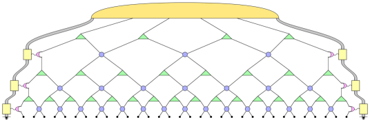
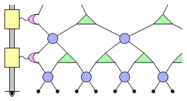
Figure 1: Left panel - Entanglement renormalization network representation for $N=32$ sites. In the bulk the MERA structure consists of isometries and disentanglers. The boundary is represented by an additional ancillary system indicated by the grey stripe. Right panel - Alternative insertion of the boundary obtained by applying the ancilla interaction tensors (magenta crescent-moons) at the same level of the disentanglers instead of the renormalizers, as done in the left panel.

The paper is organized as follows. In Sec. II we introduce the tensor network and its main properties. In Sec. III we discuss how the expectation values of local observable can be computed. Assuming a uniform tensor structure, in the thermodynamic limit, these expectation values decay as power law. We relate the associated critical exponents to those of the corresponding two-point correlations in the bulk. In Sec. IV we discuss the boundary corrections to the ground state energy. The conclusions of our work are summarized in Sec. V.

II The tensor network

Consider a 1D lattice of $N=2^{n+2}$ spins (sites), of a given local dimension $d$, with open boundary conditions. A generic pure state of such system can be expressed as

$$|\psi^{(n)}\rangle=\sum_{\ell_{1},\ldots,\ell_{N}=1}^{d}\mathcal{T}_{\ell_{1},\ldots\ell_{N}}|\xi_{\ell_{1}}\ldots\xi_{\ell_{N}}\rangle\;,$$ (1)

with $\{|\xi_{i}\rangle\}_{i}$ a canonical basis for the single qudit and $\mathcal{T}$ a type-$\left(\begin{array}[]{c}0\\ N\end{array}\right)$ tensor. Following the prescriptions of the MERA structure mera , we assume a formal decomposition of $\mathcal{T}$ which is schematically sketched in Fig. 1. Here we use the standard graphical convention (see e.g. Ref. mera ) for which each node of the graph represents a tensor (the emerging legs of the node being its indices), while a link connecting any two nodes represents the contraction of the corresponding indices. The yellow element on the top of the figure describes a type-$\left(\begin{array}[]{c}0\\ 6\end{array}\right)$ tensor ${\cal C}$ of elements ${\cal C}_{a,\ell_{1},\ell_{2},\cdots,\ell_{4},a^{\prime}}$, that we can call hat tensor. The green triangles represent instead the same $d\times d^{2}$ renormalizer tensor $\lambda$ of type-$\left(\begin{array}[]{c}1\\ 2\end{array}\right)$ of elements ${\lambda}^{u}_{\ell_{1},\ell_{2}}$, and the blue circular elements represent the same $d^{2}\times d^{2}$ disentangler tensor $\chi$ of type-$\left(\begin{array}[]{c}2\\ 2\end{array}\right)$ of elements $\chi^{u_{1},u_{2}}_{\ell_{1},\ell_{2}}$.

At the boundary, we introduce extra tensors that couple the sites at the border with an ancillary degree of freedom represented in Fig. 1 by the thick grey strip. These new elements form the lateral edges of the network and describe the boundary at each level of the MERA, i.e. at each level of the renormalization flow. As shown in the figure, each of them can be viewed as a matrix product state (yellow squares) whose bonding dimensions coincide with the coordinate space of the ancillas, which is coupled to the bulk via local coupling-elements (drawn as magenta crescent-moons in the figure). Via purification, we can always choose the dimension of such ancilla to be large enough so that the resulting interaction is described by a unitary operator, that we indicate as $\alpha$, a type-$\left(\begin{array}[]{c}2\\ 2\end{array}\right)$ tensor of elements $\alpha^{u_{1},u_{2}}_{\ell_{1},\ell_{2}}$. Similarly to the case of the $\lambda$s and of the $\chi$s, we will also assume these elements to be uniform in the network (possibly allowing the ones on the left-hand-side of the structure to differ from the ones on the right-hand-side footbcco ).

As customary with MERA-like configurations, to enforce efficient evaluation of local observables and correlation functions, the various elements of the network are assumed to obey specific contraction rules (a detailed analysis of the efficiency requirements for MERA can be found in Refs. mera ; EVE ; Giovannetti:2009p1563 ). In particular the renormalizers and the disentanglers obey isometric and unitary constraints respectively, i.e.

$$\sum_{k_{1},k_{2}}\lambda^{u}_{k_{1},k_{2}}\bar{\lambda}_{\ell}^{k_{1},k_{2}}=\delta^{u}_{\ell},\quad\sum_{k_{1},k_{2}}\chi^{u_{1},u_{2}}_{k_{1},k_{2}}\bar{\chi}_{\ell_{1},\ell_{2}}^{k_{1},k_{2}}=\delta^{u_{1}}_{\ell_{1}}\;\delta^{u_{2}}_{\ell_{2}},$$ (2)

where $\delta^{u}_{\ell}$ is the Kronecker delta, while $\bar{\lambda}_{\ell}^{u_{1},u_{2}}\equiv({\lambda}^{\ell}_{u_{1},u_{2}})^{*}$ and $\bar{\chi}_{\ell_{1},\ell_{2}}^{u_{1},u_{2}}\equiv({\chi}^{\ell_{1},\ell_{2}}_{u_{1},u_{2}})^{*}$ are the adjoint counterparts of the $\lambda$ and $\chi$ tensors respectively, obtained by exchanging their lower and upper indices and taking the complex conjugate. Similar conditions are imposed also for the edge tensors

$$\sum_{k_{1},k_{2}}\alpha^{u_{1},u_{2}}_{k_{1},k_{2}}\bar{\alpha}_{\ell_{1},\ell_{2}}^{k_{1},k_{2}}=\delta^{u_{1}}_{\ell_{1}}\;\delta^{u_{2}}_{\ell_{2}}.$$ (3)

These rules are graphically represented in Fig. 2. Finally to ensure proper state normalization, the tensor ${\cal C}$ is supposed to satisfy the identity $\sum_{a,k_{1},\cdots,k_{4},a^{\prime}}{\cal C}_{a,k_{1},\cdots,k_{4},a^{\prime}}\bar{\cal C}^{a,k_{1},\cdots,k_{4},a^{\prime}}=1$.

It is worth noticing that, by simply re-arranging the various tensorial components, an entanglement renormalization configuration which differs from the one given in Fig. 1 can be obtained. In fact, the ancilla interaction tensors $\alpha$ (the magenta crescents) can be applied at the same level of the disentanglers, instead of the renormalizers (see Fig. 1 right panel). Despite their different appearance, it can be shown that these two structures are formally equivalent to each other. This can be verified by grouping together the edge-ancilla interaction with the nearest linked element belonging to the lower half-level. Now, by just performing a polar decomposition HORN , we obtain a structure of the opposite type (although, the very first spin of the chain is now taken out the system and put into the ancilla, while the second one becomes the edge spin). Having acknowledged this equivalence, in the rest of the paper we will work with the structure of the left panel of Fig. 1.

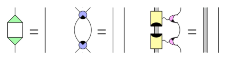
Figure 2: Rules for the elements of the tensor network of Fig. 1. The black marks drawn upon the tensors are used to make distinction between top and bottom. The first two schemes correspond to the the contractions of Eq. (2), while the last one represents the unitary constraint for the edge elements of the tensor.

III Local averages in the presence of a boundary

In the presence of the boundary, the average of any local observable depends on the distance from the boundary itself. For a one-dimensional critical system, the case we consider here, the space-dependence will be a power-law characterized by a set of critical exponents. In this Section we show how to compute local averages and how to extract these exponents.

Consider a family ${\cal F}\equiv\{|\psi^{(n)}\rangle;n=2,3,\cdots\}$ of states $|\psi^{(n)}\rangle$ of increasing sizes, described by homogeneous networks of the form shown in Fig. 1, each sharing the same structural elements (renormalizer, disentangler, edge-ancilla interaction, hat). For such family we want to calculate the expectation value of a general observable acting on a small group of neighboring sites located at a given distance from the closest edge of the system, say the left one. For instance, in the case of a three-sited observable $\Theta_{\ell}$ acting on the sites $\ell,\ell+1$, and $\ell+2$ MOTA we have

$$\langle\Theta_{\ell}\rangle^{(n)}\equiv\langle\psi^{(n)}|\Theta_{\ell}|\psi^{(n)}\rangle=\text{Tr}[\Theta_{\ell}\cdot\rho^{(n)}_{\ell,\ell+1,\ell+2}],$$ (4)

where the site indices are counted starting from the leftmost spin as the first one, and where $\rho^{(n)}_{\ell,\ell+1,\ell+2}$ is the reduced density matrix of $|\psi^{(n)}\rangle$ associated with the selected spins.

We assume a uniform MERA structure. This assumption may seem an over-simplification for a system which is not translational invariant, but it turns out that it naturally accounts for the underlying (boundary) conformal invariance. From the locality requirements imposed in Fig. 2, it is straightforward to verify that for all $1\leqslant\ell\leqslant 2^{n+1}-2$ and $n\geqslant 1$, the following recursion rules apply:

$$\begin{array}[]{c}\rho^{(n)}_{2\ell,2\ell+1,2\ell+2}=\mathcal{D}_{L}\left(\rho^{(n-1)}_{\ell,\ell+1,\ell+2}\right)\;,\\ \\ \rho^{(n)}_{2\ell+1,2\ell+2,2\ell+3}=\mathcal{D}_{R}\left(\rho^{(n-1)}_{\ell,\ell+1,\ell+2}\right)\;,\end{array}$$ (5)

where $\rho^{(n-1)}_{\ell,\ell+1,\ell+2}$ and $\rho^{(n-1)}_{\ell,\ell+1,\ell+2}$ are 3-sites reduced density matrices of $|\psi^{(n-1)}\rangle\in{\cal F}$. In these expressions, $\mathcal{D}_{L}$ and $\mathcal{D}_{R}$ are completely positive trace preserving (CPT) maps that depend only on the bulk elements of the network (indeed they coincide with the $\mathcal{D}_{L}$ and $\mathcal{D}_{R}$ maps of an ordinary homogenous MERA with the same $\lambda$ and $\chi$ jova08 ) and whose formal expression is graphically depicted in Fig. 3.

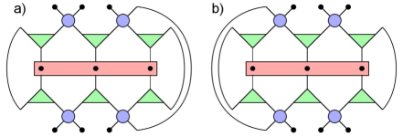
Figure 3: Sketch of the CPT maps a) $\mathcal{D}_{L}$ and b) $\mathcal{D}_{R}$; the contracted tensors picture represents their Kraus decomposition.

By means of the the renormalization procedure implied by Eq. (5), at each application of the map the site over which the average is performed approaches the boundary in an exponential fashion. Correspondingly the network depth decreases linearly. Upon reaching the boundary one has to define further operations:

$$\rho^{(n)}_{1,2,3}=\mathcal{K}_{L}\left(\rho^{(n-1)}_{A,1,2}\right)\;,$$ (6)

where $A$ refers to the degree of freedom belonging to the ancillary system, and $\mathcal{K}_{L}$ is again a CPT map, sketched in Fig. 4 (left). At this point the causal cone of the ancilla jointed with the first two sites is stable. Indeed one has

$$\rho^{(n)}_{A,1,2}=\mathcal{B}_{L}\left(\rho^{(n-1)}_{A,1,2}\right),$$ (7)

where $\mathcal{B}_{L}$ is the CPT map represented in Fig. 4 (right). Analogously to $\mathcal{B}_{L}$ and $\mathcal{K}_{L}$, we define the CPT maps at the right boundary from the mirror images of Fig. 4 and we call them $\mathcal{B}_{R}$ and $\mathcal{K}_{R}$ respectively.

Because of the stability of the causal cone mera ; EVE ; Giovannetti:2009p1563 , approaching the thermodynamical limit we can determine the reduced density matrix in proximity of the boundary by calculating the fixed point of $\mathcal{B}_{L}$. This is unique provided that the CPT map is mixing NJP ; jova08 , i.e.

$$\lim_{n\to\infty}\rho^{(n)}_{A,1,2}=\rho^{f}_{A,1,2}=\mathcal{B}_{L}\left(\rho^{f}_{A,1,2}\right).$$ (8)

We can now use this argument to obtain the expectation value in Eq. (4) for infinite volume. The resulting expression becomes particularly simple when $\mathcal{D}_{L}=\mathcal{D}_{R}=\mathcal{D}$. In this case indicating the integer part of $\log_{2}\ell$ with $\lfloor\log_{2}\ell\rfloor$, we have

$$\langle\Theta_{\ell}\rangle^{(\infty)}=\text{Tr}\left[\Theta\cdot\mathcal{D}^{\lfloor\log_{2}\ell\rfloor}\circ\mathcal{K}_{L}(\rho^{f}_{A,1,2})\right]\;,$$ (9)

where “$\circ$” stands for super-operator composition and where ${\cal D}^{\tau}$ describe a $\tau$ reiterated applications of the map ${\cal D}$.

We can now exploit the Jordan block decomposition HORN to simplify further this expression.

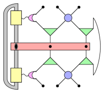
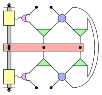
Figure 4: Tensor graph representations of the CPT map $\mathcal{K}_{L}$ (left) and $\mathcal{B}_{L}$ (right) defined in Eq. (6) and (7) respectively.

Adapting the derivation for the bulk in Ref.  Giovannetti:2009p1563 to the boundary case, we easily get

$$\langle\Theta_{\ell}\rangle^{(\infty)}=\sum_{\kappa}\kappa^{\lfloor\log_{2}\ell\rfloor}\;{g}_{\kappa}(\lfloor\log_{2}\ell\rfloor)\;,$$ (10)

where the sum spans over the eigenvalues $\kappa$ of $\mathcal{D}$ and ${g}_{\kappa}(\cdot)$ is a (finite degree) polynomial in its main argument with coefficients which depends on $\rho^{f}_{A,1,2}$ and $\mathcal{D}$. Since CPT maps are contractive, the values of $\kappa$ entering in Eq. (10) belong to the unit circle (i.e. $|\kappa|\leqslant 1$). Furthermore, if $\mathcal{D}$ is mixing (which is a reasonable assumption jova08 ) then its spectrum admits a unique eigenvector (the fix point $\rho^{f}$ of the channel) associated with $\kappa=1$; all the remaining eigenvalues have modulus strictly smaller than $1$. Under these circumstances, in the limit of large distance from the boundary, the quantity $\langle\Theta_{\ell}\rangle^{(\infty)}$ converges toward its bulk limit which is obtained by computing the expectation value of $\Theta$ on the fix point of the channel, i.e. $\langle\Theta_{\text{bulk}}\rangle^{(\infty)}=\mbox{Tr}[\Theta\rho_{f}]$. The deviations from such limiting expression can be evaluated by keeping the largest contribution associated with the terms with $\kappa\neq 1$. This yields an exponential decay in $\log_{2}\ell$ of the form

$$\langle\Theta_{\ell}\rangle^{(\infty)} = \langle\Theta_{\text{bulk}}\rangle^{(\infty)}+\sum_{\kappa\neq 1}\kappa^{\lfloor\log_{2}\ell\rfloor}\;{g}_{\kappa}(\lfloor\log_{2}\ell\rfloor)$$ (11)

$$= \langle\Theta_{\text{bulk}}\rangle^{(\infty)}+\ell^{\log_{2}|\bar{\kappa}|}\;g^{\prime}(\log_{2}\ell)\;,$$

where $\bar{\kappa}$ is the eigenvalue of $\mathcal{D}$ which has the largest absolute value smaller than one and which contributes not trivially to Eq. (10), and where $g^{\prime}(\log_{2}\ell)$ is instead some complicated function which is dominated by a polynomial of $\log_{2}\ell$. In particular, if $\Theta$ is an eigenvector of the Heisenberg adjoint of the channel $\mathcal{D}$, then Eq. (11) yields an exact power-law decay (without polynomial corrections), i.e.

$$\langle\Theta_{\ell}\rangle^{(\infty)} = c\;\kappa^{\lfloor\log_{2}\ell\rfloor}\;,$$ (12)

where $c=\;\mbox{Tr}[\Theta\;{\cal K}_{L}(\rho_{A,1,2}^{f})]$, and where $\kappa$ is the associated eigenvalue (notice that for such a $\Theta$ one has $\langle\Theta_{\text{bulk}}\rangle^{(\infty)}=0$). The above expressions show that the quantities $-\log_{2}|{\kappa}|$ play the role of the critical exponents of the system. It is now evident that these critical exponents are the half of the corresponding ones for two-point correlation functions computed in the bulk, a well-known result in conformal field theory cardy-05 . For instance fixing the distance $\Delta\ell=2^{m}$ of the two points, the bulk connected correlation function has been computed jova08 , and it holds

$$\mathfrak{C}^{(n)}_{\Delta\ell}\equiv\frac{1}{N}\sum_{\ell=1}^{N}[\langle\Theta_{\ell}\,\Theta_{\ell+\Delta\ell}\rangle^{(n)}-\langle\Theta_{\ell}\rangle^{(n)}\langle\Theta_{\ell+\Delta\ell}\vphantom{\sum}\rangle^{(n)}]$$

$$=\mbox{Tr}[(\Theta\otimes\Theta)\;\cancel{\mathcal{D}}^{\log_{2}\Delta\ell}(\sigma)]=\sum_{\xi\neq 1}\xi^{\log_{2}\Delta\ell}\;h_{\xi}(\log_{2}\Delta\ell),$$ (13)

where the summation is performed over the eigenvalues $\xi$ of the CPT map $\cancel{\mathcal{D}}=\frac{1}{2}\left(\mathcal{D}_{L}\otimes\mathcal{D}_{L}+\mathcal{D}_{R}\otimes\mathcal{D}_{R}\right)$, and where $h_{\xi}(\cdot)$ is a polynomial function of its argument (in this expression $\sigma$ stands for a traceless operator while finally $N=2^{n+2}$ is the size of the associated homogeneous MERA with periodic boundary conditions). The result then follows by noticing that by construction $\cancel{\mathcal{D}}=\mathcal{D}\otimes\mathcal{D}$ so that the $\xi$ can be expressed as products $\kappa\kappa^{\prime}$ of the eigenvalues of $\mathcal{D}$. In particular if as in Eq. (12), $\Theta$ is an eigenvector the Heisenberg adjoint of $\mathcal{D}$ we have that $\Theta\otimes\Theta$ is an eigenvector of the adjoint of $\cancel{\mathcal{D}}$ at the eigenvalue $\xi=\kappa^{2}$ and thus,

$$\mathfrak{C}^{(n)}_{\Delta\ell}=c^{\prime}\kappa^{2\log_{2}\Delta\ell}=c^{\prime}\;(\Delta\ell)^{2\log_{2}\kappa}\;,$$ (14)

which proves the claim (here $c^{\prime}=\mbox{Tr}[(\Theta\otimes\Theta)\sigma]$).

IV Boundary contribution to the ground state energy

In the presence of a boundary, the average of extensive observables (the ground state energy for example) does contain a bulk and a boundary contribution (negligible in the thermodynamic limit). In this section, we evaluate the density of the ground-state energy for a local Hamiltonian (with interactions among sites at maximum distance $\nu$) of the form

$$\mathcal{H}=\frac{1}{L-\nu+1}\sum_{j=1}^{L-\nu+1}H_{j\ldots j+\nu},$$ (15)

where $\nu$ is the number of sites involved in the model interaction $H$. While this problem is easily solved in a level-recursive manner for a MERA structure (in which periodic boundary conditions hold), when explicit conditions over a defined boundary are involved things become slightly more complicated.

Suppose, for simplicity, that the interaction is again a $\nu=$ 3-body operator, therefore

$$\langle\mathcal{H}\rangle=\text{Tr}[H_{3}\cdot\bar{\rho}_{3}^{(n)}]\;,$$ (16)

where

$$\bar{\rho}_{3}^{(n)}\equiv\frac{1}{2^{n+2}-2}\sum_{j=1}^{2^{n}}\rho^{(n)}_{j,j+1,j+2}\;\;.$$

We need to build a recursive function which relates this average density matrix to the one belonging to the previous tensor level $\bar{\rho}_{3}^{(n-1)}$. Of course, the boundaries will play some role too in this relation

$$\bar{\rho}_{3}^{(n)}=\frac{1}{2^{n+2}-2}\left[\mathcal{K}_{L}\left(\rho^{(n-1)}_{A,1,2}\right)+\mathcal{K}_{R}\left(\rho^{(n-1)}_{2^{n+1}-1,2^{n+1},A^{\prime}}\right)\right]\\ +\left(1-\frac{1}{2^{n+1}-1}\right)\cdot\mathcal{D}\left(\bar{\rho}_{3}^{(n-1)}\right),$$ (17)

(here $\mathcal{D}$ is the average of $\mathcal{D}_{L}$ and $\mathcal{D}_{R}$). This equation shows the contributions of both bulk and edge terms; nevertheless, when we approach the thermodynamical limit $n\to\infty$, the contribution of the first two terms vanishes in every norm, because any density matrix has trace norm bounded by one and CPT maps are contractive.

This means that the extensive influence of the boundary upon the lattice grows slower than the size of the system, a physical sounding and known property. To quantitatively describe such behavior, we compute the (total) energy associated with the block of the first $2^{\tau}-1$ spins near a boundary, say the left one. In our notation this corresponds to

$$E^{(n)}_{1\ldots 2^{\tau}-1}=\text{Tr}\left[H_{3}\cdot\sum_{j=1}^{2^{\tau}-1}\rho^{(n)}_{j,j+1,j+2}\right].$$ (18)

Exploiting the usual formalism of level-growing CPT maps, we can rewrite the sum in (18) as

$$\sum_{j=1}^{2^{\tau}-1}\rho^{(n)}_{j,j+1,j+2}=\sum_{p=0}^{\tau-1}\,2^{p}\cdot\mathcal{D}^{p}\circ\mathcal{K}_{L}\circ\mathcal{B}_{L}^{\tau-p-1}\left(\rho^{(n-\tau)}_{A,1,2}\right).$$ (19)

Now, we can successfully approach the thermodynamical limit while keeping $\tau$ fixed. Recalling that $\rho^{f}_{A,1,2}$ is the fixed point of $\mathcal{B}_{L}$, we obtain

$$E^{(\text{th})}_{1\ldots 2^{\tau}-1}=\text{Tr}\left[H_{3}\cdot\sum_{p=0}^{\tau-1}\,2^{p}\;\mathcal{D}^{p}\circ\mathcal{K}_{L}\left(\rho^{f}_{A,1,2}\right)\right].$$ (20)

As expected, the result diverges for $\tau\to\infty$ since the series is made of terms growing in trace norm. To explicitly estimate how this quantity deviates from its corresponding value in the bulk as $\tau$ grows we evaluate the following quantity

$$\Delta E^{(\text{th})}_{1\ldots 2^{\tau}-1}=-(2^{\tau}-1)\;\text{Tr}\left[H_{3}\cdot\rho^{f}_{3}\right]+\\ +\text{Tr}\left[H_{3}\cdot\sum_{p=0}^{\tau-1}\,2^{p}\;\mathcal{D}^{p}\circ\mathcal{K}_{L}\left(\rho^{f}_{A,1,2}\right)\right]=\\ =\text{Tr}\left[H_{3}\cdot\sum_{p=0}^{\tau-1}\,2^{p}\;\mathcal{D}^{p}\left\{\mathcal{K}_{L}\left(\rho^{f}_{A,1,2}\right)-\rho^{f}_{3}\right\}\right].$$ (21)

Notice that in this case the map $\mathcal{D}$ applies to a traceless operator, therefore if we decompose the argument in a basis of generalized eigenvectors for $\mathcal{D}$, it must have null component over the unique state of eigenvalue one. As a result the boundary contribution to the ground state energy has the form

$$\Delta E^{(\text{th})}_{1\ldots\infty}=\sum_{\kappa_{D}\neq 1}\;\sum_{p=0}^{\infty}(2\kappa_{\mathcal{D}})^{p}\cdot g_{\kappa_{\mathcal{D}}}(p),$$ (22)

where $g(\cdot)$ is a polynomial in its main argument. Looking at Eq. (22), we notice that the inner sum diverges for any eigenvalue $\kappa_{\mathcal{D}}$ of $\mathcal{D}$ greater or equal to $1/2$, unless the $g$ are identically zero for such values of $\kappa_{\mathcal{D}}$. In general this will happen when $\rho^{f}_{3}-\mathcal{K}_{L}(\rho^{f}_{A,1,2})$ has null component over any generalized eigenspace whose $\kappa_{\mathcal{D}}\geq 1/2$.

Interestingly enough the capability of such deviation to diverge is another manifestation that the MERA states of Fig. 1 are critical: indeed only the integral of a power-law function can diverge, while for an exponential decaying correlation function the integral of the corresponding action is always finite.

V Conclusions

In this paper we exploited the properties of MERA to describe boundary critical phenomena. We considered the case of a one-dimensional critical system with a boundary. To this end we modified the local structure of the MERA at the boundary to account for more flexibility in its description.

Besides showing how to compute local observables, we achieved two main results. First of all we showed, as predicted by boundary conformal field theory, that the critical exponents associated to the decay of the one-point function (as a function of the distance from the boundary) is always half of the one of the bulk two-point correlation function corresponding to the same scaling operator. Secondly we compute the boundary corrections to the ground state energy and determined its scaling behavior. As in the bulk case, also in the presence of the boundary, most of the critical properties are determined solely by the eigenvalues of the MERA transfer matrix.

A remarkable feature of treating boundary critical phenomena with MERAs is that it is enough to consider uniform tensor network. This is the result of the scale invariance of the underlying tensor network which holds also in the presence of boundaries. In addition to the practical advantage in the numerical simulations, this observation further clarifies the properties of the MERA. It is worth noticing that such property (that is at the basis of the effectiveness of a bounded MERA) is physically equivalent to the fact that, in boundary critical phenomena, the operator content of the bulk is not influenced by the boundary bcs , suggesting that maybe the connection between MERA and general renormalization group theory is deeper than what nowadays understood.

One dimensional systems display the peculiar feature that the boundary can be critical only when also the bulk is. This is not the case in higher dimensions bcs , where we can have a critical boundary in a gapped system, resulting in a richer scenario for the boundary-bulk phase diagram. This richness will reflect in the possibility to have different compositions of tensor structure. In this paper we considered a matrix product state (at the border) connected to a MERA. It is easy to imagine that, to describe critical surfaces in a non-critical bulk, different compositions of tensor networks are required.

During the writing of this work a paper by G. Evenbly et al. appeared on the archive discussing boundary critical phenomena using MERA, see Ref. BOU .

We acknowledge fruitful discussions with M. Campostrini, S. Montangero and M. Rizzi, and financial support from FIRB-RBID08B3FM and the National Research Foundation and Ministry of Education Singapore.

References

- (1) F. Verstraete, J.I. Cirac, V. Murg, Adv. Phys. 57, 143 (2008); J. I. Cirac and F. Vestraete, J. Phys. A 42, 504004 (2009).
- (2) S. R. White, Phys. Rev. Lett. 69, 2863 (1992); Phys. Rev. B 48, 10345 (1993); U. Schollwoeck, Rev. Mod. Phys. 77, 259 (2005).
- (3) M. Fannes, B. Nachtergaele, and R. F. Werner, Lett. Math. Phys. 25, 249 (1992); S. Ostlund and S. Rommer, Phys. Rev. Lett. 75, 3537 (1995); G. Vidal, Phys. Rev. Lett. 91, 147902 (2003); F. Verstraete, D. Porras, and J. I. Cirac, Phys. Rev. Lett. 93, 227205 (2004).
- (4) F. Verstraete, J. I. Cirac, Eprint arXiv:cond-mat/0407066; V. Murg, F. Verstraete, and J. I. Cirac, Phys. Rev. A 75, 033605 (2007).
- (5) W. Dür et al., Phys. Rev. Lett. 94, 097203 (2005); S. Anders et al., Phys. Rev. Lett. 97, 107206 (2006).
- (6) G. Vidal, Phys. Rev. Lett. 99, 220405 (2007); ibid. 101, 110501 (2008); 0912.1651.
- (7) L. Cincio, J. Dziarmaga, M. M. Rams, Phys. Rev. Lett. 100, 240603 (2008).
- (8) G. Evenbly and G. Vidal, Phys. Rev. Lett. 102 180406 (2009).
- (9) P. Corboz, G. Evenbly, F. Verstraete, and G. Vidal, arXiv:0904.4151.
- (10) V. Giovannetti, S. Montangero, and R. Fazio, Phys. Rev. Lett. 101, 180503 (2008).
- (11) R. N. C. Pfeifer, G. Evenbly, and G. Vidal, Phys. Rev. A 79, 04030 (2009); G. Evenbly, P.Corboz, and G. Vidal, 0912.2166.
- (12) V. Giovannetti, S. Montangero, M. Rizzi, and R. Fazio, Phys Rev A 79 052314 (2009).
- (13) S. Montangero, M. Rizzi, V. Giovannetti, and R. Fazio, Phys. Rev. B 80, 113103 (2009).
- (14) K. Binder, in Phase Transitions and Critical Phenomena, edited by C. Domb and J. L. Lebowitz (Academic Press, London, 1983) Vol. 8, p. 1; H. W. Diehl, in Phase Transitions and Critical Phenomena, edited by C. Domb and J. L. Lebowitz (Academic Press, London, 1986), Vol. 10, p. 75.
- (15) J. L. Cardy, Nucl. Phys. B 240 514 (1984); Nucl. Phys. B 275, 200 (1986); Boundary Conformal Field Theory, in Encyclopedia of Mathematical Physics, ed J.-P. Francoise, G. Naber, and S. Tsun Tsou, (Elsevier, Amsterdam, 2006) [hep-th/0411189].
- (16) H. Saleur, Lectures on Non Perturbative Field Theory and Quantum Impurity Problems, cond-mat/9812110; I. Affleck, N. Laflorencie, and E. S. Sorensen, J. Phys. A 42, 504009 (2009).
- (17) P. Calabrese and J. Cardy, Phys. Rev. Lett. 96, 136801(2006); J. Stat. Mech. (2007) P06008; J. Stat. Mech. (2007) P10004.
- (18) W. Werner, Springer Lecture Notes in Mathematics 1180, 113 (2004); W. Kager and B. Nienhuis, J. Stat. Phys. 115, 1149 (2004); J. Cardy, Annals Phys. 318, 81 (2005); M. Bauer and D. Bernard, Phys. Rep. 432, 115 (2006).
- (19) Notice that allowing the boundary elements to change along the renormalization flow corresponds to introduce a boundary condition changing operator cardy-05 in the language of CFT.
- (20) G. Evenbly and G. Vidal Phys. Rev. B 79, 144108 (2009).
- (21) R. A. Horn and C. R. Johnson, Matrix Analysis (Cambridge: Cambridge University Press) (1990).
- (22) The three-side observable is the simplest configuration we can consider since the three-site causal cone is the smallest stable for a MERA-like bulk mera .
- (23) D. Burgarth and V. Giovannetti, New J. Phys. 9, 150 (2007).
- (24) G. Evenbly, R. N. C. Pfeifer, V. Pico, S. Iblisdir, L. Tagliacozzo, I. P. McCulloch, and G. Vidal, arXiv:0912.1642v1 [cond-mat.str-el].