Matching between typical fluctuations and large deviations in disordered systems :
application to the statistics of the ground state energy in the SK spin-glass model

Abstract

For the statistics of global observables in disordered systems, we discuss the matching between typical fluctuations and large deviations. We focus on the statistics of the ground state energy $E_{0}$ in two types of disordered models : (i) for the directed polymer of length $N$ in a two-dimensional medium, where many exact results exist (ii) for the Sherrington-Kirkpatrick spin-glass model of $N$ spins, where various possibilities have been proposed. Here we stress that, besides the behavior of the disorder-average $E_{0}^{av}(N)$ and of the standard deviation $\Delta E_{0}(N)\sim N^{\omega_{f}}$ that defines the fluctuation exponent $\omega_{f}$, it is very instructive to study the full probability distribution $\Pi(u)$ of the rescaled variable $u=\frac{E_{0}(N)-E_{0}^{av}(N)}{\Delta E_{0}(N)}$ : (a) numerically, the convergence towards $\Pi(u)$ is usually very rapid, so that data on rather small sizes but with high statistics allow to measure the two tails exponents $\eta_{\pm}$ defined as $\ln\Pi(u\to\pm\infty)\sim-|u|^{\eta_{\pm}}$. In the generic case $1<\eta_{\pm}<+\infty$, this leads to explicit non-trivial terms in the asymptotic behaviors of the moments $\overline{Z_{N}^{n}}$ of the partition function when the combination $[|n|N^{\omega_{f}}]$ becomes large (b) simple rare events arguments can usually be found to obtain explicit relations between $\eta_{\pm}$ and $\omega_{f}$. These rare events usually correspond to ’anomalous’ large deviation properties of the generalized form $R(w_{\pm}=\frac{E_{0}(N)-E_{0}^{av}(N)}{N^{\kappa_{\pm}}})\sim e^{-N^{\rho_{\pm}}{\cal R}_{\pm}(w_{\pm})}$ (the ’usual’ large deviations formalism corresponds to $\kappa_{\pm}=1=\rho_{\pm}$).

I Introduction

In the field of disordered systems, the interest has been first on self-averaging quantities, like the free-energy per degree of freedom, or other thermodynamic observables that determine the phase diagram. However, it has become clear over the years that a true understanding of random systems has to include the sample-to-sample fluctuations of global observables, in particular in disorder-dominated phases where interesting universal critical exponents show up. Besides these typical sample-to-sample fluctuations, it is natural to characterize also the large deviations properties, since rare anomalous regions are known to play a major role in various properties of random systems.

Among the various global observables that are interesting, the simplest one is probably the ground-state energy $E_{0}$ of a disordered sample. Since it is the minimal value among the energies of all possible configurations, the study of its distribution belongs to the field of extreme value statistics. Whereas the case of independent random variables is well classified in three universality classes [1], the problem for the correlated energies within a disordered sample remains open and has been the subject of many recent studies (see for instance [2] and references therein). For many-body models with $N$ degrees of freedom ($N$ spins for disordered spin models, $N$ monomers for disordered polymers models), the interest lies

(i) in the scaling behavior of the average $E_{0}^{av}(N)$ and the standard deviation $\Delta E_{0}(N)$ with $N$. Following the definitions of Ref. [3], the ‘shift exponent’ $\omega_{s}$ governs the correction to extensivity of the averaged value

$$E_{0}^{av}(N)\simeq Ne_{0}+N^{\omega_{s}}e_{1}+...$$ (1)

whereas the ‘fluctuation exponent’ $\omega_{f}$ governs the growth of the standard deviation

$$\Delta E_{0}(N)\sim N^{\omega_{f}}$$ (2)

(ii) in the asymptotic distribution $\Pi(u)$ of the rescaled variable

$$u\equiv\frac{E_{0}-E_{0}^{av}(N)}{\Delta E_{0}(N)}$$ (3)

in the limit $N\to\infty$

$${\cal P}_{N}(E_{0})\mathop{\simeq}_{N\to\infty}\frac{1}{\Delta E_{0}(N)}\ \Pi\left(u=\frac{E_{0}-E_{0}^{av}(N)}{\Delta E_{0}(N)}\right)$$ (4)

This scaling function $\Pi(u)$ describes the typical events where the variable $u$ is finite.

(iii) in the large deviations properties. In the standard ’large deviation formalism’ (see for instance the recent review [4] and references therein), one is interested in the exponentially rare events giving rise to a finite difference $v$ between the intensive observable $(E_{0}/N)$ and its averaged value $E_{0}^{av}(N)/N$

$$v\equiv\frac{E_{0}-E_{0}^{av}(N)}{N}$$ (5)

In disordered systems, the probability distributions of these rare events is not necessarily exponentially small in $N$ but can sometimes involve other exponents $\gamma_{\pm}$ (see examples below in the text)

$$D^{-}_{N}(v_{-}\equiv\frac{E_{0}-E_{0}^{av}(N)}{N}<0) \mathop{\simeq}_{N\to\infty}e^{-N^{\gamma_{-}}{\cal D}_{-}(v_{-})}$$

$$D^{+}_{N}(v_{+}\equiv\frac{E_{0}-E_{0}^{av}(N)}{N}>0) \mathop{\simeq}_{N\to\infty}e^{-N^{\gamma_{+}}{\cal D}_{+}(v_{+})}$$ (6)

In this paper, we discuss these properties for two types of disordered models : for the directed polymer of length $N$ in a two-dimensional medium, where many exact results exist, and for the Sherrington-Kirkpatrick (SK) spin-glass model of $N$ spins, where various possibilities have been proposed from numerical results or theoretical arguments. The main conclusions we draw from these two cases are the following :

(a) it is very instructive to study the tails of the full probability distribution $\Pi(u)$ of Eq. 4 : these tails are usually described by the following form

$$\ln\Pi(u) \mathop{\propto}_{u\to-\infty}-(-u)^{\eta_{-}}+...$$

$$\ln\Pi(u) \mathop{\propto}_{u\to+\infty}-u^{\eta_{+}}+...$$ (7)

where the two tails exponents $\eta_{\pm}$ are usually different and in the range $1\leq\eta_{\pm}\leq+\infty$. In particular, the very common fits based on generalized Gumbel distributions are very restrictive and very misleading since they correspond to the unique values $\eta_{-}=1$ and $\eta_{+}=+\infty$. We also discuss the consequences of Eq. 7 for the moments $\overline{Z_{N}^{n}}$ of order $n$ (either positive or negative) of the partition function $Z_{N}$ at very low temperature.

(b) simple rare events arguments can usually be found to obtain explicit relations between $\eta_{\pm}$ and $\omega_{f}$. The probability distributions of these rare events usually correspond to ’anomalous’ large deviation properties of the generalized forms

$$R^{-}_{N}(w_{-}\equiv\frac{E_{0}-E_{0}^{av}(N)}{N^{\kappa_{-}}}<0) \mathop{\simeq}_{N\to\infty}e^{-N^{\rho_{-}}{\cal R}_{-}(w_{-})}$$

$$R^{+}_{N}(w_{+}\equiv\frac{E_{0}-E_{0}^{av}(N)}{N^{\kappa_{+}}}>0) \mathop{\simeq}_{N\to\infty}e^{-N^{\rho_{+}}{\cal R}_{+}(w_{+})}$$ (8)

The paper is organized as follows. In Section II, we recall the exact results concerning the directed polymer in a two-dimensional random medium, and discuss their meaning for the above points (a) and (b). In Section III, we discuss the case of the Sherrington-Kirkpatrick spin-glass model, and we present numerical results obtained for small sizes but with high statistics. Our conclusions are summarized in section IV.

II Reminder on the directed polymer in a two-dimensional random medium

II.1 Brief summary of exact results

The directed polymer model in a two-dimensional random medium (see the review [5]) is an exactly soluble model that has the following properties :

(i) a single exponent [6, 7, 8, 9]

$$\omega_{s}=\omega_{f}=\frac{1}{3}$$ (9)

governs both the correction to extensivity of the average $E_{0}^{av}(N)$ (Eq. 1) and the width $\Delta E_{0}(N)$ (Eq. 2).

(ii) the rescaled distribution $\Pi(u)$ of Eq. 4 is the Tracy-Widom distribution of the largest eigenvalue of random matrices ensembles [8, 9, 10]. In particular, the two tails exponents of Eq. 7 read

$$\eta_{-} =\frac{3}{2}$$

$$\eta_{+} =3$$ (10)

(iii) the exponents of the large deviations forms of Eq. 6 are respectively [11, 12, 13, 14]

$$\gamma_{-} =1$$

$$\gamma_{+} =2$$ (11)

After this brief reminder of known results, we now turn to their physical interpretation.

II.2 Physical interpretation of the large deviation exponents in terms of simple rare events

As explained in detail in [14], the large deviation exponents of Eq. 10 can be understood as follows

(-) to obtain a ground state energy which is extensively lower than the typical, it is sufficient to draw $N$ anomalously good on-site energies along the ground state path. This will happen with a probability $e^{-(cst)N}$ corresponding to $\gamma_{-}=1$ of Eq. 11.

(+) to obtain a ground state energy which is extensively higher than the typical, one needs to draw $N^{2}$ bad on-site energies (i.e. in the whole sample). This will happen with a probability $e^{-(cst)N^{2}}$ corresponding to $\gamma_{+}=2$ of Eq. 11.

Note that in the Asymmetric Exclusion process language, the interpretation is that to slow down the traffic, it is sufficient to slow down a single particle, whereas to speed up the traffic, one needs to speed up all particles [11]. In the random matrix language, the interpretation is that to push the maximal eigenvalue inside the Wigner sea, one needs to reorganize everything, whereas to pull the maximal eigenvalue outside the Wigner sea, one may leave the Wigner sea unchanged for the other eigenvalues [12, 13].

The fact that these large deviation exponents $\gamma_{\pm}$ can be guessed via simple physical arguments is an important lesson that is very useful in other disordered models which are not exactly solvable : in particular, these arguments can be easily extended to the directed polymer in a random medium of higher dimensionality [14], or to other observables in various models [14, 15, 16].

II.3 Matching between typical fluctuation and large deviations

For an arbitrary probability distribution, the typical fluctuations in the bulk and the rare fluctuations in the far tails are in general different questions. However, for the probability distribution of the ground state energy $E_{0}(N)$ (or more generally the probability distributions of other global observables) in disordered statistical physics models, it is very natural, from a physical point of view, to expect some matching between the typical fluctuation scaling regime where $E_{0}-E_{0}^{av}\sim N^{\omega_{f}}$ and the large deviations scaling regime where $E_{0}-E_{0}^{av}\sim N$. More precisely, the tails in the regions $u\to\pm\infty$ of the rescaled distribution $\Pi(u)$ of typical fluctuations should match smoothly the large deviation region regime where the variable $v$ of Eq. 5 is finite, which corresponds to the regime where the variable $u$ of Eq. 3 is of order $u\propto N^{1-\omega_{f}}$. If one plugs this scaling into the asymptotic form of Eq. 7, and if one insists that one should then recover the large deviations exponents of Eq. 6, one obtains the very simple relations between exponents [14]

$$(1-\omega_{f})\eta_{\pm}=\gamma_{\pm}$$ (12)

For the directed polymer in a two-dimensional random medium, these relations are satisfied by the values quoted in Eqs 9,10 and 11. This smooth matching has also been discussed in the equivalent problems concerning the current in the asymmetric exclusion process [11] and the largest eigenvalue of Gaussian random matrices [12, 13].

This matching property between typical fluctuation and large deviations is again an important lesson that can be used in other disordered models which are not exactly solvable. These relations have been checked in detail for the directed polymer in dimension $d=2,3$ [17] as well as on hierarchical lattices [14]. This matching property has also been used recently for the distribution of the dynamical barriers [15, 16]. It is also interesting from a physical point of view, because the asymmetry $\eta_{-}<\eta_{+}$ seen in the distribution of typical events can be seen as a consequence of the asymmetry of rare events $\gamma_{-}<\gamma_{+}$.

II.4 Consequences for the moments of the partition function

Since a direct calculation of the probability distribution of the ground state of a disordered model is usually very difficult, analytical calculations usually focus on the moments $\overline{Z^{n}_{N}}$ of the partition function $Z_{N}$. Then one can use two types of arguments to relate the distribution of $Z_{N}=e^{-\beta F_{N}}$ to the distribution $P_{N}(E_{0})$ of the ground state energy $E_{0}(N)$ : (1) at very low temperature $T\to 0$, the partition function will be dominated by the ground state $Z_{N}(\beta\to+\infty)\simeq e^{-\beta E_{0}(N)}$ (2) moreover in some models, where the disorder-dominated phase $0\leq T<T_{c}$ is governed by a zero-temperature fixed point, one expects that in the whole region of temperatures $0\leq T<T_{c}$, the probability distribution of the free-energy $F_{N}$ will actually have the same properties as the distribution of $E_{0}$. Since (2) is valid for the directed polymer model, but cannot be taken for granted in all disordered models, we will restrict here to the point of view (1) of very low temperature $T\to 0$.

There exists a simple argument that has been proposed by Zhang [5] on the specific case on the directed polymer, that relates the scaling behaviors of the moments $\overline{Z^{n}_{N}}$ with the size $N$ and with the replica index $n$ to the properties of $P_{N}(E_{0})$. The idea is to evaluate the moments by using the rescaled distribution of Eq. 4

$$\overline{Z_{N}^{n}}=\int dE_{0}P_{N}(E_{0})e^{-\beta nE_{0}}\simeq\frac{1}{\Delta E_{0}(N)}e^{-\beta nE_{0}^{av}(N)}\ \int du\Pi(u)e^{-\beta n\Delta E_{0}(N)u}$$ (13)

For the case $n>0$ considered by Zhang [5], the integral can be then evaluated by a saddle point method in the region $u\to-\infty$, where one may use the asymptotic behavior of Eq. 7 with the exponent $\eta_{-}>1$ : the saddle point is of order

$$u^{*}\propto(\beta n\Delta E_{0}(N))^{\frac{1}{\eta_{-}-1}}$$ (14)

that should be large $u^{*}\gg 1$, and one obtains

$$\overline{Z_{N}^{n>0}}\propto e^{-\beta nE_{0}^{av}(N)+(cst)(\beta n\Delta E_{0}(N))^{\frac{\eta_{-}}{\eta_{-}-1}}}$$ (15)

For the case $n<0$, the equivalent calculation yields in term of the other tail exponent $\eta_{+}>1$ :

$$\overline{Z_{N}^{n<0}}\propto e^{-\beta nE_{0}^{av}(N)+(cst)(\beta(-n)\Delta E_{0}(N))^{\frac{\eta_{+}}{\eta_{+}-1}}}$$ (16)

For the directed polymer in a two-dimensional random medium, one obtains, using $\Delta E_{0}(N)\propto N^{\omega_{f}}$ with the explicit values of Eqs 9,10

$$\overline{Z_{N}^{n>0}}\propto e^{-\beta nE_{0}^{av}(N)+(cst)(\beta n)^{3}N}$$ (17)

where one recognizes the combination $(n^{3}N)$ that appears in the Bethe Ansatz replica calculation of Ref. [7]. Moreover, in Zhang’s argument [5], one actually imposes that the non-trivial term of Eq. 15 should be extensive in $N$ (because for positive integer $n$, the moments of the partition function can be formulated in terms of the iteration of some transfer matrix, and thus they have to diverge exponentially in $N$ with some Lyapunov exponent) to obtain the relation $\omega_{f}\frac{\eta_{-}}{\eta_{-}-1)}=1$ (which is equivalent here to the relation of Eq. 12 obtained previously by the rare event interpretation).

For $n<0$, the obtained behavior

$$\overline{Z_{N}^{n<0}}\propto e^{-\beta nE_{0}^{av}(N)+(cst)(\beta(-n))^{\frac{3}{2}}N^{\frac{1}{2}}}$$ (18)

is rather different : the only extensive contribution of order $N$ in the exponential comes from $E_{0}^{av}(N)$. The leading contribution due to fluctuations is only of subleading order $N^{\frac{1}{2}}$, and it involves a non-integer power of the replica index $(-n)$. To the best of our knowledge, the behavior of these negative moments has not been much discussed in the literature, in contrast to the case $n>0$.

These saddle-point calculations based on the facts that the tails exponents satisfy $\eta_{\pm}>1$ can be very useful in other non-exactly soluble models, for instance in the Sherrington-Kirkpatrick spin-glass model that we now consider.

III Sherrington-Kirkpatrick spin-glass model

For short-ranged spin-glasses in any finite dimension $d$, it has been proven that the fluctuation exponent of Eq. 2 is exactly $\theta_{f}=d/2$ [18]. Accordingly, the rescaled distribution ${\Pi}(u)$ of Eq. (4) was numerically found to be Gaussian in $d=2$ and $d=3$ [3], suggesting some Central Limit theorem. On the contrary, in mean-field spin-glasses, the width does not grows as $N^{1/2}$ and the distribution is not Gaussian, as will be discussed in more details in this section. Studies on long-ranged one-dimensional spin-glasses [19] have confirmed that non-mean-field models are characterized by Gaussian distributions, whereas mean-field models are not.

III.1 Brief summary of previous works

The statistics of the ground state energy of the Sherrington-Kirkpatrick spin-glass model [20]

$$H=-\sum_{1\leq i<j\leq N}J_{ij}S_{i}S_{j}$$ (19)

where the couplings $J_{ij}$ are random quenched variables of zero mean $\overline{J}=0$ and of variance $\overline{J^{2}}=1/N$, has been much studied recently with the following outputs :

(i) there seems to be a consensus (see for instance [21, 3, 22] and references therein) on the shift exponent of Eq. 1

$$\omega_{s}=\frac{1}{3}$$ (20)

whereas the ‘fluctuation exponent’ $\omega_{f}$ is still under debate between the value (see [23, 3, 22] and references therein)

$$\omega_{f}=\frac{1}{4}$$ (21)

and the value (see [24, 25, 21, 26] and references therein)

$$\omega_{f}=\frac{1}{6}$$ (22)

(ii) the asymptotic distribution $\Pi(u)$ of Eq. 4 has been measured numerically by various authors (see [21, 28, 27] and references therein), but unfortunately it has almost always been fitted by ’generalized Gumbel distributions’ of the form $e^{m(u-e^{u})}$ containing a single free-parameter $m$ for the shape. However these fits are very restrictive and very misleading since the tails exponents are fixed to be

$${\rm GeneralizedGumbel:}\ \ \eta_{-} =1$$

$$\ \eta_{+} =+\infty$$ (23)

for any value of the parameter $m$. In this paper, we propose instead that these exponents are in the range $1<\eta_{\pm}<+\infty$.

(iii) the large deviation properties have been also very controversial. In [29], numerical results have been interpreted with the following values for the exponents $\gamma_{\pm}$ of Eq. 6

$${\rm Ref.[29]:}\ \ \gamma_{-} \simeq 1.2$$

$$\gamma_{+} \simeq 1.5$$ (24)

Other proposals are (see [26] and references therein)

$${\rm Ref.[26]:}\ \ \gamma_{-} =1$$

$$\gamma_{+} =2$$ (25)

After this brief summary of conflicting proposals, we now turn to the analysis along the same line as in the previous section concerning the directed polymer model.

III.2 Discussion of simple rare events

The simplest rare events one may consider for the SK model are the following :

(-) to obtain a ground state energy which is much lower than the typical, it is natural to consider the anomalous ferromagnetic samples [29] that appear with a small probability of order $e^{-(cst)N^{2}}$ (one needs to draw $N^{2}$ positive couplings in Eq. 19), and that will corresponds to anomalously low energy of order $E_{0}\propto-(cst)N^{3/2}$. These events corresponds to the ’very large deviation’ of the generalized form of Eq. 8 with the values [29]

$${\rm Ferro:}\ \ \rho_{-} =2$$

$$\ \ \ \ \kappa_{-} =\frac{3}{2}$$ (26)

This form has been checked numerically in [29].

(+) to obtain a ground state energy which is much higher than the typical, one could consider the anomalous antiferromagnetic samples that appear with a small probability of order $e^{-(cst)N^{2}}$ (one needs to draw $N^{2}$ negative couplings) and that will give an energy extensively higher. In the large deviation form of Eq. 6, this would corresponds to

$${\rm Antiferro:}\ \ \gamma_{+}=2$$ (27)

This value corresponds to the proposal of Eq. 25 from Ref. [26], but disagrees with the numerical proposal of Eq. 24 from Ref. [29]. The question is whether to obtain an extensively higher energy, it is sufficient to draw anomalously only a number of order $N^{1.5}$ random couplings instead of $N^{2}$. We are presently not aware of any simple argument in favor of this smaller power $N^{1.5}$.

III.3 Matching between typical fluctuation and large deviations

In the (+) region, the matching between typical fluctuation and rare events leads to the same relation as in Eq. 12

$$(1-\omega_{f})\eta_{+}=\gamma_{+}$$ (28)

In particular, the possible values of $\gamma_{+}$ and $\omega_{f}$ leads to the following values for the tail exponent $\eta_{+}$ :

$${\rm If}\ \ \gamma_{+}=2\ \ :\eta_{+}^{\left(\omega_{f}=\frac{1}{4}\right)} =\frac{8}{3}=2.6666..$$

$$\eta_{+}^{\left(\omega_{f}=\frac{1}{6}\right)} =\frac{12}{5}=2.4$$ (29)

or

$${\rm If}\ \ \gamma_{+}=\frac{3}{2}\ \ :\eta_{+}^{\left(\omega_{f}=\frac{1}{4}\right)} =2$$

$$\eta_{+}^{\left(\omega_{f}=\frac{1}{6}\right)} =\frac{9}{5}=1.8$$ (30)

In the (-) region, the matching between typical fluctuation and the very large deviations of Eq. 24 leads to the relation

$$\left(\kappa_{-}-\omega_{f}\right)\eta_{-}=\rho_{-}$$ (31)

Using the values of Eq. 26 one obtains the two possible values for $\eta_{-}$

$${\rm If}\ \ \ \omega_{f}=\frac{1}{4}\ \ :\eta_{-} =\frac{8}{5}=1.6$$

$${\rm If}\ \ \ \omega_{f}=\frac{1}{6}\ \ \eta_{-} =\frac{3}{2}=1.5$$ (32)

If this matching works, the region of large deviation of Eq. 6 which is between the typical region and the very large deviation region, is constrained by consistency to involve the exponent

$$\gamma_{-}=\left(1-\omega_{f}\right)\eta_{-}$$ (33)

The two possible values read

$${\rm If}\ \ \ \omega_{f}=\frac{1}{4}\ \ :\gamma_{-} =\frac{6}{5}=1.2$$

$${\rm If}\ \ \ \omega_{f}=\frac{1}{6}\ \ :\gamma_{-} =\frac{5}{4}=1.25$$ (34)

Both are close to the numerical value of Eq. 24 proposed by Ref. [29]. Both disagree with the value $\gamma_{-}=1$ of Eq. 25 used in replica calculations of [26].

III.4 Consequences for the moments of the partition function

As explained in detail in section II.4, the moments of the partition function $Z_{N}$ are then expected to follow Eqs 15 and 16

$$\overline{Z_{N}^{n>0}} \propto e^{-\beta nE_{0}^{av}(N)+(cst)(\beta nN^{\omega_{f}})^{\frac{\eta_{-}}{\eta_{-}-1}}}$$

$$\overline{Z_{N}^{n<0}} \propto e^{-\beta nE_{0}^{av}(N)+(cst)(\beta(-n)N^{\omega_{f}})^{\frac{\eta_{+}}{\eta_{+}-1}}}$$ (35)

For positive $n>0$ : the two possible values of $\omega_{f}$ and of the associated tail exponent $\eta_{-}$ (see Eq. 32) correspond to the behaviors

$${\rm If}\ \ \ \omega_{f}=\frac{1}{4}\ \ :\overline{Z_{N}^{n>0}} \propto e^{-\beta nE_{0}^{av}(N)+(cst)(\beta nN^{\frac{1}{4}})^{\frac{8}{3}}}$$

$${\rm If}\ \ \ \omega_{f}=\frac{1}{6}\ \ :\overline{Z_{N}^{n>0}} \propto e^{-\beta nE_{0}^{av}(N)+(cst)(\beta nN^{\frac{1}{6}})^{3}}$$ (36)

We note that in both cases, the non-trivial part is sub-extensive in $N$, in contrast to the replica calculations of [26], but in agreement with the replica calculations of [30, 31]. It is also clear that the non-trivial part $(n^{3}N^{1/2})$ for the case $\omega_{f}=\frac{1}{6}$, is simpler than the term $(n^{8/3}N^{2/3})$ for the case $\omega_{f}=\frac{1}{4}$. In both cases, the powers of $n$ that appear are different from the value $n^{5}$ of perturbative replica calculations [32, 26].

For negative $n<0$ : for the case $\gamma_{+}=2$ of Eq. 29, the possible behaviors are

$${\rm If}\ \ \ \omega_{f}=\frac{1}{4}\ \ :\overline{Z_{N}^{n<0}} \propto e^{-\beta nE_{0}^{av}(N)+(cst)(\beta(-n)N^{\frac{1}{4}})^{\frac{8}{5}}}$$

$${\rm If}\ \ \ \omega_{f}=\frac{1}{6}\ \ :\overline{Z_{N}^{n<0}} \propto e^{-\beta nE_{0}^{av}(N)+(cst)(\beta(-n)N^{\frac{1}{6}})^{\frac{12}{7}}}$$ (37)

For the case $\gamma_{+}=3/2$ of Eq. 24 proposed in Ref. [29], the behavior of the moments can be similarly evaluated using Eq. 30. Again in all cases, the non-trivial part is sub-extensive in $N$, as already proposed in [33]. Concerning the powers of $(-n)$, the exponent $(12/7)$ for the case $\omega_{f}=\frac{1}{6}$ is in agreement with the replica calculations of [26].

III.5 Numerical results for small sizes and large statistics of samples

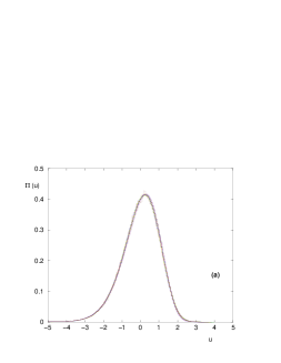
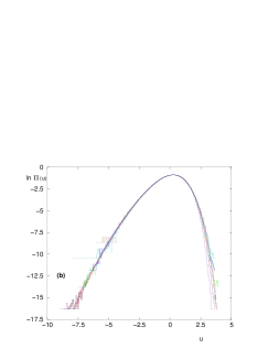
Figure 1: Rescaled probability distribution of the ground state energy $E_{0}(N)$ in the SK model : (a) the histograms $\Pi_{N}(u)$ of the rescaled variable $u$ of Eq. 3 measured for even sizes in the range $6\leq N\leq 20$ almost coincide : this shows that the convergence in $N$ towards the asymptotic form is very rapid. (b) same data in log-scale to see the tails : one sees that the left tail does not change, whereas finite-size effects are visible on the right tail.

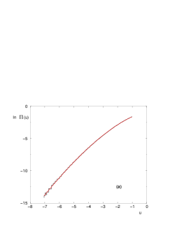
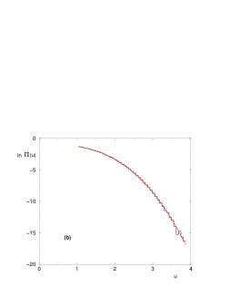
Figure 2: Tails exponents of the rescaled distribution $\Pi_{N}(u)$ : examples of fits of our numerical rescaled histogram (step function) corresponding to the size $N=10$ (a) The smooth curve corresponds to the best three-parameter fit in the range $u\leq-1$ by the form $(a_{0}-a_{1}(-u)^{\eta_{-}})$ : the left tail exponent is of order $\eta_{-}\simeq 1.5$. (b) The smooth curve corresponds to the best three-parameter fit in the range $u\geq 1$ by the form $(a_{0}-a_{1}u^{\eta_{+}})$ : the right tail exponent is of order $\eta_{+}\simeq 2.8$.

Most numerical works on the distribution of the ground state energy in the SK model have followed the strategy to study the biggest sizes $N$ as possible, to measure the averaged value and the variance (see [21, 3, 22] and references therein). An opposite strategy has been followed in Ref. [27] where an exact enumeration of the disordered samples with the binomial distribution $\pm J$ was performed for small sizes. As mentioned in [22], the results for the rescaled distribution $\Pi(u)$ at $N=9$ are already very good when compared to the results for larger $N$. In other cases, we have also found that the distribution of rescaled variables converge much more rapidly than other observables [15, 16, 34]. In the following, we thus follow the same strategy : we study the distribution of $E_{0}(N)$ for the small sizes with a high statistics of disordered samples.

On Fig. 1 (a), we show the measured histograms $\Pi_{N}(u)$ of the the rescaled variable $u$ of Eq. 3 for even sizes in the range $6\leq N\leq 20$ with a statistics of $2.10^{8}\geq n_{s}(N)\geq 13.10^{4}$ disordered samples : one clearly sees that all these histograms almost coincide. Our conclusion is thus that the convergence in $N$ towards the asymptotic form is very rapid, so that these small-size data should provide a reliable measure of the asymptotic $\Pi(u)$. As explained before, we are mainly interested into the tails exponents $\eta_{\pm}$ of Eq. 7 : as shown on Fig. 1 (b) the convergence of the left tail is extremely good, whereas the convergence of the right tail presents much stronger finite-size effects.

Let us first consider the left tail. The three-parameter fit of $\Pi(u)$ in the range $u\leq-1$ by the form $(a_{0}-a_{1}(-u)^{\eta_{-}})$ yields the value (see Fig 2 (a))

$$\eta_{-}\simeq 1.5$$ (38)

that corresponds exactly to the value associated to $\omega_{f}=1/6$ (see Eq. 32). Of course, it is probably not far enough from the alternative value $\eta_{-}=1.6$ corresponding to $\omega_{f}=1/4$ (see Eq. 32) to really rule out the value $\omega_{f}=1/4$.

Let us now turn to the right tail. The three-parameter fit of $\Pi(u)$ in the range $u\geq 1$ by the form $(a_{0}-a_{1}u^{\eta_{+}})$ yields values for $\eta_{+}$ that are less precise, as a consequence of the finite-size effects visible on Fig. 1 (b). We have already found in other studies that the right tail is usually more difficult to measure than the left tail [14]. Nevertheless our non-precise values of $\eta_{+}$ in the range $[2.4,2.9]$ (see Fig 2 (b)) seem more compatible with the value $\gamma_{+}=2$ than with the value $\gamma_{+}=1.5$ (see Eq. 29 and 30).

III.6 Final discussion

In summary, even if a definitive agreement on the precise value of the fluctuation exponent $\omega_{f}$ remains difficult to reach (see [21, 3, 22] and references therein), our conclusions concerning the SK model are the following :

(i) the numerical measure of the left tail exponent $\eta_{-}$ is in agreement with the matching argument based on rare ferromagnetic samples described by the very-large deviation form of Eq. 8 with the values of Eq. 26 from Ref. [29]. Then the large deviation form of Eq. 6 is constrained to involve an exponent $\gamma_{-}$ given by Eq. 33

$$\gamma_{-}=(1-\omega_{f})\eta_{-}=\frac{2(1-\omega_{f})}{(\frac{3}{2}-\omega_{f})}$$ (39)

This explains the numerical value of Eq. 24 proposed in Ref. [29], and excludes the value $\gamma_{-}=1$ of Eq. 25 used in the replica calculations of [26]. We note moreover that this ’usual large deviation value’ $\gamma_{-}=1$ would be satisfied only for the value $\omega_{f}=1/3$, i.e. only if the fluctuation exponent $\omega_{f}$ would coincide with the shift exponent $\omega_{s}=1/3$ of Eq. 20.

(ii) although less precise, the numerical measure of the right tail exponent $\eta_{+}$ is more in favor of the large deviation exponent $\gamma_{+}=2$, that can be justified with a simple rare events argument (see Eq. 27).

(iii) finally, the facts that the tails exponents satisfy $\eta_{\pm}>1$ induces non-trivial behavior for the moments of the partition function (see Eqs. 35) when $(|n|N^{\omega_{f}})$ becomes large. In particular, from Eqs 36 and 37, our conclusion is that the only extensive term in $N$ comes from the trivial term $E_{0}^{av}(N)$ both for negative and positive $n$. Moreover, the non-trivial sub-extensive terms can a priori involve non-integer powers of the replica index $n$.

IV Conclusion

In this paper, we have discussed the statistics of the ground state energy $E_{0}(N)$ in two types of disordered models: (i) for the directed polymer of length $N$ in a two-dimensional medium, where many exact results exist (ii) for the Sherrington-Kirkpatrick spin-glass model, where various possibilities are still under debate both numerically and theoretically. Our main conclusions are the following. Besides the behavior of the disorder-average $E_{0}^{av}(N)$ and of the standard deviation $\Delta E_{0}(N)\sim N^{\omega_{f}}$, it is very instructive to study the full probability distribution $\Pi(u)$ of the rescaled variable $u=\frac{E_{0}(N)-E_{0}^{av}(N)}{\Delta E_{0}(N)}$ :

(a) numerically, the convergence towards $\Pi(u)$ is usually very rapid, so that data on rather small sizes but with high statistics allow to measure the tails exponents $\eta_{\pm}$ that satisfy generically $1<\eta_{\pm}<+\infty$ (whereas the very common fits based on generalized Gumbel distributions correspond to the unique values $\eta_{-}=1$ and $\eta_{+}=+\infty$). Moreover, if one wishes to measure tails beyond the region probed via simple sampling, one may uses a Monte-Carlo procedure in the disorder, as done in [28] for the SK model, and in [17] for the directed polymer model.

(b) simple rare events arguments can usually be found to obtain explicit relations between $\eta_{\pm}$ and $\omega_{f}$. These rare events usually correspond to ’anomalous’ large deviation properties of the generalized form $R_{N}(w_{\pm}=\frac{E_{0}(N)-E_{0}^{av}(N)}{N^{\kappa_{\pm}}})\sim e^{-N^{\rho_{\pm}}{\cal R}_{\pm}(w_{\pm})}$ (the ’usual” large deviations formalism corresponding to $\kappa_{\pm}=1=\rho_{\pm}$ is too restrictive for disordered models, as shown on explicit examples in the text).

(c) We have also discussed the consequences of $1<\eta_{\pm}<+\infty$ for the moments $\overline{Z_{N}^{n}}$ of order $n$ (either positive or negative) of the partition function $Z_{N}$. In the regime where $[|n|N^{\omega_{f}}]$ becomes large, a saddle-point calculation leads to explicit non-trivial terms in the asymptotic behaviors of the moments $\overline{Z_{N}^{n}}$ of the partition function.

We have shown in detail how this analysis for the directed polymer is in agreement with all known exact results. For the SK model, we have explained how this analysis agrees or disagrees with various possibilities debated in the literature.

In conclusion, we believe that this type of analysis based on the matching between typical fluctuations and rare events is very useful to study disordered systems. Here we have focused on the statistics of the ground state energy, but it can also be used for other global observables such as the maximal dynamical barrier of a disordered sample [15, 16], or for the statistics of large excitations in ferromagnets and spin-glasses [14].

References

- [1] E.J. Gumbel, “ Statistics of extreme” (Columbia University Press, NY 1958); J. Galambos, “ The asymptotic theory of extreme order statistics” ( Krieger , Malabar, FL 1987).
- [2] G. Biroli, J.P. Bouchaud and M. Potters, J. Stat. Mech. P07019 (2007).
- [3] J.-P. Bouchaud, F. Krzakala and O.C. Martin, Phys. Rev. B68, 224404 (2003).
- [4] H. Touchette, Phys. Rep. 478, 1 (2009).
- [5] T. Halpin-Healy and Y.-C. Zhang, Phys. Repts., 254, 215 (1995).
- [6] D. A. Huse, C. L. Henley, and D. S. Fisher, Phys. Rev. Lett. 55, 2924 (1985).
- [7] M. Kardar, Nucl. Phys. B 290 582 (1987).
- [8] K. Johansson, Comm. Math. Phys. 209 (2000) 437.
- [9] M. Prahofer and H. Spohn, Physica A 279, 342 (2000) ; M. Prahofer and H. Spohn, Phys. Rev. Lett. 84, 4882 (2000) ; M. Prahofer and H. Spohn, J. Stat. Phys. 108, 1071 (2002).
- [10] M. Prähoher and H. Spohn, http://www-m5.ma.tum.de/KPZ/.
- [11] B. Derrida and J.L. Lebowitz, Phys. Rev. Lett. 80, 209 (1998)
- [12] D.S. Dean and S.N. Majumdar, Phys. Rev. Lett. 97, 160201 (2006) and Phys. Rev. E 77, 041108 (2008).
- [13] S. N. Majumdar and M. Vergassola, Phys. Rev. Lett. 102, 060601 (2009).
- [14] C. Monthus and T. Garel, J. Stat. Mech. (2008) P01008.
- [15] C. Monthus and T. Garel, arXiv:0910.4833.
- [16] C. Monthus and T. Garel, arXiv:0911.5649.
- [17] C. Monthus and T. Garel, Phys. Rev. E 74, 051109 (2006).
- [18] J. Wehr and M. Aizenman, J. Stat. Phys. 60 (1990) 287.
- [19] H.G. Katzgraber, M. Körner, F. Liers, M. Jünger and A.K. Hartmann, Phys. Rev. B 72, 094421 (2005).
- [20] D. Sherrington and S. Kirkpatrick, Phys. Rev. Lett. 35, 1792 (1975).
- [21] M. Palassini, cond-mat/0307713; M. Palassini, J. Stat. Mech. P10005 (2008).
- [22] S. Boettcher, arxiv:0906.1292.
- [23] T. Aspelmeier, M.A. Moore and A.P. Young, Phys. Rev. Lett. 90, 127202 (2003).
- [24] A. Crisanti, G. Paladin, H.J. Sommers and A. Vulpiani, J. Phys. I France 2, 1325 (1992).
- [25] T. Aspelmeier, A. Billoire, E. Marinari and M.A. Moore, J. Phys. A Math. Theor. 41 , 324008 (2008).
- [26] G. Parisi and T. Rizzo, Phys. Rev. Lett. 101, 117205 (2008) and Phys. Rev. B 79, 134205 (2009) and arXiv:0901.1100.
- [27] S. Boettcher and T.M. Kott, Phys. Rev. B 72, 212408 (2005).
- [28] M. Körner, H.G. Katzgraber and A.K. Hartmann, J. Stat. Mech., P04005 (2006).
- [29] A. Andreanov, F. Barbieri and O.C. Martin, Eur. Phys. J. B 41, 365 (2004).
- [30] T. Aspelmeier and M.A. Moore, Phys. Rev. Lett. 90, 177201 (2003).
- [31] C. De Dominicis ans P. Di Francesco, J. Phys. A Math. Gen. 36, 10955 (2003).
- [32] I. Kondor, J. Phys. A Math Gen 16, L127 (1983).
- [33] V. Dotsenko, S. Franz and M. Mézard, J. Phys. A 27 , 2351 (1994).
- [34] C. Monthus and T. Garel, J. Phys. A: Math. Theor. 41 (2008) 255002; C. Monthus and T. Garel, J. Stat. Mech. (2008) P07002 ; C. Monthus and T. Garel, J. Phys. A: Math. Theor. 41 (2008) 375005.