Variational Bayesian inference and complexity control for stochastic block models

Abstract: It is now widely accepted that knowledge can be acquired from networks by clustering their vertices according to connection profiles. Many methods have been proposed and in this paper we concentrate on the Stochastic Block Model (SBM). The clustering of vertices and the estimation of SBM model parameters have been subject to previous work and numerous inference strategies such as variational Expectation Maximization (EM) and classification EM have been proposed. However, SBM still suffers from a lack of criteria to estimate the number of components in the mixture. To our knowledge, only one model based criterion, ICL, has been derived for SBM in the literature. It relies on an asymptotic approximation of the Integrated Complete-data Likelihood and recent studies have shown that it tends to be too conservative in the case of small networks. To tackle this issue, we propose a new criterion that we call ILvb, based on a non asymptotic approximation of the marginal likelihood. We describe how the criterion can be computed through a variational Bayes EM algorithm.

Key words: Random graphs, Stochastic block models, Community detection, Variational EM, Variational Bayes EM, Integrated complete-data likelihood, Integrated observed-data likelihood

Received: date / Accepted: date

1 Introduction

Networks are used in many scientific fields such as biology (Albert and Barabási 2002) and social sciences (Snijders and Nowicki 1997, Nowicki and Snijders 2001). They aim at modelling with edges the way objects of interest are related to each other. Examples of such data sets are friendship (Palla et al 2007), protein-protein interaction networks (Barabási and Oltvai 2004), powergrids (Watts and Strogatz 1998) and the Internet (Zanghi et al 2008). In this context, a lot of attention has been paid on developing models to learn knowledge from the network topology. It appears that available methods can be grouped into three significant categories.

Some models look for community structure, also called homophily or assortative mixing (Girvan and Newman 2002, Danon et al 2005). Given a network, the vertices are partitioned into classes such that vertices of a class are mostly connected to vertices of the same class. In the model of Handcock et al (2007), which extends Hoff et al (2002), vertices are clustered depending on their positions in a continuous latent space. They proposed a two-stage maximum likelihood approach and a Bayesian algorithm, as well as an asymptotic BIC criterion to estimate the number of latent classes. The two-stage maximum likelihood approach first maps the vertices in the latent space and then uses a mixture model to cluster the resulting positions. In practice, this procedure converges quickly but looses some information by not estimating the positions and the cluster model at the same time. Conversely, the Bayesian algorithm, based on Markov Chain Monte Carlo, estimates both the latent positions and the mixture model parameters simultaneously. It gives better results but is time consuming. Both the maximum likelihood and the Bayesian approach are implemented in the R package “latentnet” (Krivitsky and Handcock 2009).

Other models look for disassortative mixing, in which vertices mostly connect to vertices of different classes (Estrada and Rodriguez-Velazquez 2005). They are particularly suitable for the analysis of bipartite networks which are used in numerous applications. Examples of data sets having such structures are transcriptional regulatory networks where operons encode transcription factors directly involved in operons regulation. To get some insight into the transcription process, these two types of nodes are often grouped into different classes with high inter connection probabilities. Other examples are citation networks where authors cite or are cited by papers. For a more detailed description of the differences between community structure and disassortative mixing, see Newman and Leicht (2007).

Finally, a few models can look for both community structure and disassortative mixing. Hofman and Wiggins (2008) proposed a probabilistic framework, as well as an efficient clustering algorithm. Their model, implemented in the software “VBMOD”, is based on two key parameters $\lambda$ and $\epsilon$. Given a network, it assumes that vertices connect with probability $\lambda$ if they belong to the same class and with probability $\epsilon$ otherwise. Moreover, they introduced a non asymptotic Bayesian criterion to estimate the number of classes. It is based on a variational approximation of the marginal likelihood and has shown promising results. In this paper, we focus on the Stochastic Block Model (SBM) which was originally developed in social sciences (White et al 1976, Fienberg and Wasserman 1981, Frank and Harary 1982, Holland et al 1983, Snijders and Nowicki 1997). Given a network, SBM assumes that each vertex belongs to a hidden class among $Q$ classes, and uses a $Q\times Q$ matrix $\operatorname{\boldsymbol{\pi}}$ to describe the intra and inter connection probabilities. Moreover, the class proportions are represented using a $Q$-dimensional vector $\operatorname{\boldsymbol{\alpha}}$. No assumption is made on the form of the connectivity matrix such that very different structures can be taken into account. In particular, SBM can characterize the presence of hubs which make networks locally dense (Daudin et al 2008). Moreover and to some extent, it generalizes many of the existing graph clustering techniques as shown in Newman and Leicht (2007). For instance, the model of Hofman and Wiggins (2008) can be seen as a constrained SBM where the diagonal of $\operatorname{\boldsymbol{\pi}}$ is set to $\lambda$ and all the other elements to $\epsilon$.

Many methods have been proposed in the literature to jointly estimate SBM model parameters and cluster the vertices of a network. They all face the same difficulty. Indeed, contrary to many mixture models, the conditional distribution of all the latent variables $\operatorname{{\bf Z}}$ and model parameters, given the observed data $\operatorname{{\bf X}}$, can not be factorized due to conditional dependency (for more details, see Daudin et al 2008). Therefore, optimization techniques such as the EM algorithm can not be used directly. Nowicki and Snijders (2001) proposed a Bayesian probabilistic approach. They introduced some prior Dirichlet distributions for the model parameters and used Gibbs sampling to approximate the posterior distribution over the model parameters and posterior predictive distribution. Their algorithm is implemented in the software BLOCKS, which is part of the package StoCNET (Boer et al 2006). It gives accurate a posteriori estimates but can not handle networks with more than 200 vertices. Daudin et al (2008) proposed a frequentist variational EM approach for SBM which can handle much larger networks. Online strategies have also been developed (Zanghi et al 2008).

While many inference strategies have been proposed for estimation and clustering purpose, SBM still suffers from a lack of criteria to estimate the number of classes in networks. Indeed, many criteria, such as the Bayesian Information Criterion (BIC) or the Akaike Information Criterion (AIC) (Burnham and Anderson 2004) are based on the likelihood $p(\operatorname{{\bf X}}|\operatorname{\boldsymbol{\alpha}},\operatorname{\boldsymbol{\pi}})$ of the observed data $\operatorname{{\bf X}}$, which is intractable here. To tackle this issue, Mariadassou et al (2010) and Daudin et al (2008) used a criterion, so-called ICL, based on an asymptotic approximation of the integrated complete-data likelihood. This criterion relies on the joint distribution $p(\operatorname{{\bf X}},\operatorname{{\bf Z}}|\operatorname{\boldsymbol{\alpha}},\operatorname{\boldsymbol{\pi}})$ rather than $p(\operatorname{{\bf X}}|\operatorname{\boldsymbol{\alpha}},\operatorname{\boldsymbol{\pi}})$ and can be easily computed, even in the case of SBM. ICL was originally proposed by Biernacki et al (2000) for model selection in Gaussian mixture models, and is known to be particularly suitable for cluster analysis view since it favors well separated clusters. However, because it relies on an asymptotic approximation, Biernacki et al (2010) showed, in the case of mixtures of multivariate multinomial distributions, that it may fail to detect interesting structures present in the data, for small sample sizes. Mariadassou et al (2010) obtained similar results when analyzing networks generated using SBM. They found that this asymptotic criterion tends to underestimate the number of classes when dealing with small networks. We emphasize that, to our knowledge, ICL is currently the only model based criterion developed for SBM.

Our main concern in this paper is to propose a new criterion for SBM, based on the marginal likelihood $p(\operatorname{{\bf X}})$, also called integrated observed-data likelihood. The marginal likelihood is known to focus on density estimation view and is expected to provide a consistent estimation of the distribution of the data. For a more detailed overview of the differences between integrated complete-data likelihood and integrated observed-data likelihood, we refer to Biernacki et al (2010). In the case of SBM, the marginal likelihood is not tractable and we describe in this paper how a non asymptotic approximation can be obtained through a variational Bayes EM algorithm.

In Section 2, we describe SBM and we introduce some non informative conjugate prior distributions for the model parameters. The variational Bayes EM algorithm is then presented in Section 3. We show in Section 4 how it naturally leads to a new model selection criterion that we call ILvb, based on a non asymptotic approximation of the marginal likelihood. Finally, in Section 5, we carry out some experiments using simulated data sets and the metabolic network of Escherichia coli, to assess ILvb.

The R package “mixer” implementing this work is available from the following web site: http://cran.r-project.org.

2 A Mixture Model for Graphs

The data we model consists of a $N\times N$ binary matrix $\operatorname{{\bf X}}$, with entries $X_{ij}$ describing the presence or absence of an edge from vertex $i$ to vertex $j$. Both directed and undirected relations can be analyzed but in the following, we focus on undirected relations. Therefore $\operatorname{{\bf X}}$ is symmetric.

2.1 Model and Notations

The Stochastic Block Model (SBM) introduced by Nowicki and Snijders (2001) associates to each vertex of a network a latent variable $\operatorname{{\bf Z}}_{i}$ drawn from a multinomial distribution, such that $Z_{iq}=1$ if vertex $i$ belongs to class $q$

$$\operatorname{{\bf Z}}_{i}\sim\mathcal{M}\Big{(}1,\>\operatorname{\boldsymbol{\alpha}}=(\alpha_{1},\alpha_{2},\dots,\alpha_{Q})\Big{)}.$$

We denote $\operatorname{\boldsymbol{\alpha}}$, the vector of class proportions. The edges are then drawn from Bernoulli distribution

$$X_{ij}|\{Z_{iq}Z_{jl}=1\}\sim\mathcal{B}(\pi_{ql}),$$

where $\operatorname{\boldsymbol{\pi}}$ is a $Q\times Q$ matrix of connection probabilities. According to this model, the latent variables $\operatorname{{\bf Z}}_{1},\dots,\operatorname{{\bf Z}}_{N}$ are iid and given this latent structure, all the edges are supposed to be independent. Note that SBM was originally described in a more general setting, allowing any discrete relational data. However, as explained previously, we concentrate in the following on binary edges only.

Thus, when considering an undirected graph without self loops, this leads to

$$p(\operatorname{{\bf Z}}|\operatorname{\boldsymbol{\alpha}})=\prod_{i=1}^{N}\mathcal{M}(\operatorname{{\bf Z}}_{i};\>1,\operatorname{\boldsymbol{\alpha}})=\prod_{i=1}^{N}\prod_{q=1}^{Q}\alpha_{q}^{Z_{iq}},$$

and

$$p(\operatorname{{\bf X}}|\operatorname{{\bf Z}},\operatorname{\boldsymbol{\pi}}) =\prod_{i<j}p(X_{ij}|\operatorname{{\bf Z}}_{i},\operatorname{{\bf Z}}_{j},\operatorname{\boldsymbol{\pi}})$$

$$=\prod_{i<j}\prod_{q,l}\mathcal{B}(X_{ij}|\pi_{ql})^{Z_{iq}Z_{jl}}$$

$$=\prod_{i<j}\prod_{q,l}\left(\pi_{ql}^{X_{ij}}(1-\pi_{ql})^{1-X_{ij}}\right)^{Z_{iq}Z_{jl}}.$$

In the case of a directed graph, the products over $i<j$ must be replaced by products over $i\neq j$. The edges $X_{ii}$ must also be taken into account if the graph contains self-loops.

Note that SBM is related to the infinite block model of Kemp et al (2004) although the number $Q$ of classes is fixed. Moreover, contrary to the mixed membership stochastic block model of Airoldi et al (2008) which captures partial membership and allows each vertex to have a distribution over a set of classes, SBM assumes that each vertex of a network belongs to a single class.

The identifiability of SBM was studied by Allman et al (2009), who showed that the model is generically identifiable up to a permutation of the classes. In other words, except in a set of parameters which has a null Lebesgue’s measure, two parameters imply the same random graph model if and only if they differ only by the ordering of the classes.

2.2 A Bayesian Stochastic Block Model

SBM can be described in a full Bayesian framework where it can be considered as a generalisation of the affiliation model proposed by Hofman and Wiggins (2008). Indeed, the Bayesian model of Hofman and Wiggins (2008) considers a simple structure where vertices of the same class connect with probability $\lambda$ and with probability $\epsilon$ otherwise. Therefore, it can be seen as a constrained SBM where the diagonal of $\operatorname{\boldsymbol{\pi}}$ is set to $\lambda$ and all the other elements to $\epsilon$.

To extend the SBM frequentist model, we first specify some non informative conjugate priors for the model parameters. Since $p(\operatorname{{\bf Z}}_{i}|\operatorname{\boldsymbol{\alpha}})$ is a multinomial distribution, we consider a Dirichlet distribution for the mixing coefficients

$$p\Big{(}\operatorname{\boldsymbol{\alpha}}|\operatorname{{\bf n}}^{0}=\{n_{1}^{0},\dots,n_{Q}^{0}\}\Big{)}=\operatorname{Dir}(\operatorname{\boldsymbol{\alpha}};\>\operatorname{{\bf n}}^{0}),$$ (2.1)

where $n_{q}^{0}=1/2,\>\forall q$. This Dirichlet distribution corresponds to a non-informative Jeffreys prior distribution which is known to be proper (Jeffreys 1946). It is also possible to consider a uniform distribution on the $Q-1$ dimensional simplex by fixing $n_{q}^{0}=1,\forall q$.

Since $p(X_{ij}|\operatorname{{\bf Z}}_{i},\operatorname{{\bf Z}}_{j},\operatorname{\boldsymbol{\pi}})$ is a Bernoulli distribution, we use independent $\operatorname{Beta}$ priors to model the connectivity matrix $\operatorname{\boldsymbol{\pi}}$

$$p\Big{(}\operatorname{\boldsymbol{\pi}}|\operatorname{\boldsymbol{\eta}}^{0}=(\eta_{ql}^{0}),\operatorname{\boldsymbol{\zeta}}^{0}=(\zeta_{ql}^{0})\Big{)}=\prod_{q\leq l}\operatorname{Beta}(\pi_{ql};\>\eta_{ql}^{0},\zeta_{ql}^{0}),$$ (2.2)

with $\eta_{ql}^{0}=\zeta_{ql}^{0}=1/2,\forall q$. This corresponds to a product of non-informative Jeffreys prior distributions. Note that if the graph is directed, the products over $q\leq l$, must be replaced by products over $q,l$ since $\operatorname{\boldsymbol{\pi}}$ is no longer symmetric.

Thus, the model parameters are now seen as random variables (see Figure 1) whose distributions depend on the hyperparameters $\operatorname{{\bf n}}^{0}$, $\operatorname{\boldsymbol{\eta}}^{0}$, and $\operatorname{\boldsymbol{\zeta}}^{0}$. In the following, since these hyperparameters are fixed and in order to keep the notations simple, they will not be shown explicitly in the conditional distributions.

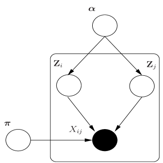
Figure 1: Directed acyclic graph representing the Bayesian view of the stochastic block model. Nodes represent random variables, which are shaded when they are observed and edges represent conditional dependencies.

3 Estimation

In this section, we first describe the variational EM algorithm used by Daudin et al (2008) to jointly estimate SBM model parameters and cluster the vertices of a network. We then propose a new variational Bayes EM algorithm for SBM which approximates the full posterior distribution of the model parameters and latent variables, given the observed data $\operatorname{{\bf X}}$. This procedure relies on a lower bound which will be later used, in Section 4, as a non asymptotic approximation of the marginal log-likelihood $\ln p(\operatorname{{\bf X}})$.

3.1 Variational Approach

The likelihood $p(\operatorname{{\bf X}}|\operatorname{\boldsymbol{\alpha}},\operatorname{\boldsymbol{\pi}})$ of the observed data $\operatorname{{\bf X}}$ can be obtained through the marginalization $p(\operatorname{{\bf X}}|\operatorname{\boldsymbol{\alpha}},\operatorname{\boldsymbol{\pi}})=\sum_{\operatorname{{\bf Z}}}p(\operatorname{{\bf X}},\operatorname{{\bf Z}}|\operatorname{\boldsymbol{\alpha}},\operatorname{\boldsymbol{\pi}})$. This summation involves $Q^{N}$ terms and quickly becomes intractable. To tackle such problem, the well known EM algorithm (Dempster et al 1977, McLachlan and Krishnan 1997) has been applied with success on a large variety of mixture models. This two stage estimation approach (Hathaway 1986, Neal and Hinton 1998) can be described in a variational inference framework. Thus, given a distribution $q(\operatorname{{\bf Z}})$ over the latent variables, the $\log$-likelihood of the observed data is decomposed into two terms

$$\ln p(\operatorname{{\bf X}}|\operatorname{\boldsymbol{\alpha}},\operatorname{\boldsymbol{\pi}})=\mathcal{L}\Big{(}q(.);\>\operatorname{\boldsymbol{\alpha}},\operatorname{\boldsymbol{\pi}}\Big{)}+\operatorname{KL}\Big{(}q(.)\>||\>p(.|\operatorname{{\bf X}},\operatorname{\boldsymbol{\alpha}},\operatorname{\boldsymbol{\pi}})\Big{)},$$ (3.1)

where

$$\mathcal{L}\Big{(}q(.);\>\operatorname{\boldsymbol{\alpha}},\operatorname{\boldsymbol{\pi}}\Big{)}=\sum_{\operatorname{{\bf Z}}}q(\operatorname{{\bf Z}})\ln\{\frac{p(\operatorname{{\bf X}},\operatorname{{\bf Z}}|\operatorname{\boldsymbol{\alpha}},\operatorname{\boldsymbol{\pi}})}{q(\operatorname{{\bf Z}})}\},$$ (3.2)

and

$$\operatorname{KL}\Big{(}q(.)\>||\>p(.|\operatorname{{\bf X}},\operatorname{\boldsymbol{\alpha}},\operatorname{\boldsymbol{\pi}})\Big{)}=-\sum_{\operatorname{{\bf Z}}}q(\operatorname{{\bf Z}})\ln\{\frac{p(\operatorname{{\bf Z}}|\operatorname{{\bf X}},\operatorname{\boldsymbol{\alpha}},\operatorname{\boldsymbol{\pi}})}{q(\operatorname{{\bf Z}})}\}.$$ (3.3)

In (3.1) and (3.3), KL denotes the Kullback-Leibler divergence between the distribution $q(\operatorname{{\bf Z}})$ and the distribution $p(\operatorname{{\bf Z}}|\operatorname{{\bf X}},\operatorname{\boldsymbol{\alpha}},\operatorname{\boldsymbol{\pi}})$. Suppose that the current value of the model parameters is $(\operatorname{\boldsymbol{\alpha}}^{old},\operatorname{\boldsymbol{\pi}}^{old})$. During the E-step, the lower bound $\mathcal{L}\Big{(}q(.);\>\operatorname{\boldsymbol{\alpha}}^{old},\operatorname{\boldsymbol{\pi}}^{old}\Big{)}$ is maximized with respect to $q(\operatorname{{\bf Z}})$ while holding the model parameters fixed. The solution to this optimization step occurs when the KL divergence vanishes, that is when $q(\operatorname{{\bf Z}})$ is equal to $p(\operatorname{{\bf Z}}|\operatorname{{\bf X}},\operatorname{\boldsymbol{\alpha}}^{old},\operatorname{\boldsymbol{\pi}}^{old})$. The lower bound is then equal to the log-likelihood of the observed data. In the M-step, the distribution $q(\operatorname{{\bf Z}})$ is held fixed and the lower bound is maximized with respect to the model parameters to give $(\operatorname{\boldsymbol{\alpha}}^{new},\operatorname{\boldsymbol{\pi}}^{new})$. This causes the log-likelihood to increase.

Unfortunately, when considering SBM, $p(\operatorname{{\bf Z}}|\operatorname{{\bf X}},\operatorname{\boldsymbol{\alpha}},\operatorname{\boldsymbol{\pi}})$ is not tractable and variational approximations are required. It can be easily verified that minimizing (3.3) with respect to $q(\operatorname{{\bf Z}})$ is equivalent to maximizing the lower bound (3.2) of (3.1) with respect to $q(\operatorname{{\bf Z}})$. To obtain a tractable algorithm, Daudin et al (2008) assumed that the distribution $q(\operatorname{{\bf Z}})$ can be factorized such that

$$q(\operatorname{{\bf Z}})=\prod_{i=1}^{N}q(\operatorname{{\bf Z}}_{i})=\prod_{i=1}^{N}\mathcal{M}(\operatorname{{\bf Z}}_{i};\>1,\operatorname{\boldsymbol{\tau}}_{i}),$$

where $\tau_{iq}$ is a variational parameter denoting the probability of node $i$ to belong to class $q$. This gives rise to a so-called variational EM procedure. During the variational E-step, the model parameters are fixed and, by maximizing (3.2) with respect to $q(\operatorname{{\bf Z}})$, the algorithm looks for an approximation of the conditional distribution of the latent variables. Conversely, during the variational M-step, the approximation $q(\operatorname{{\bf Z}})$ is fixed and the lower bound is maximized with respect to the model parameters. This procedure is repeated until convergence and was proposed by Daudin et al (2008) for the SBM model.

3.2 Variational Bayes EM

In the context of mixture models, the conditional distribution $p(\operatorname{{\bf Z}}|\operatorname{{\bf X}},\operatorname{\boldsymbol{\alpha}},\operatorname{\boldsymbol{\pi}})$ can generally be computed and therefore Bayesian inference strategies focus on estimating the posterior distribution $p(\operatorname{\boldsymbol{\alpha}},\operatorname{\boldsymbol{\pi}}|\operatorname{{\bf X}})$. The distribution $p(\operatorname{{\bf Z}},\operatorname{\boldsymbol{\alpha}},\operatorname{\boldsymbol{\pi}}|\operatorname{{\bf X}})$ is then simply given by a byproduct. However, when considering SBM, the distribution $p(\operatorname{{\bf Z}}|\operatorname{{\bf X}},\operatorname{\boldsymbol{\alpha}},\operatorname{\boldsymbol{\pi}})$ is intractable and so we propose to approximate the full distribution $p(\operatorname{{\bf Z}},\operatorname{\boldsymbol{\alpha}},\operatorname{\boldsymbol{\pi}}|\operatorname{{\bf X}})$. We follow the work of Attias (1999), Corduneanu and Bishop (2001), Svensén and Bishop (2004) on Bayesian mixture modelling and Bayesian model selection. Thus, the marginal log-likelihood, also called integrated observed-data log-likelihood, can be decomposed into two terms

$$\ln p(\operatorname{{\bf X}})=\mathcal{L}\Big{(}q(.)\Big{)}+\operatorname{KL}\Big{(}q(.)\>||\>p(.|\operatorname{{\bf X}})\Big{)},$$ (3.4)

where

$$\mathcal{L}\Big{(}q(.)\Big{)}=\sum_{\operatorname{{\bf Z}}}\int\int q(\operatorname{{\bf Z}},\operatorname{\boldsymbol{\alpha}},\operatorname{\boldsymbol{\pi}})\ln\{\frac{p(\operatorname{{\bf X}},\operatorname{{\bf Z}},\operatorname{\boldsymbol{\alpha}},\operatorname{\boldsymbol{\pi}})}{q(\operatorname{{\bf Z}},\operatorname{\boldsymbol{\alpha}},\operatorname{\boldsymbol{\pi}})}\}d\operatorname{\boldsymbol{\alpha}}d\operatorname{\boldsymbol{\pi}},$$ (3.5)

and

$$\operatorname{KL}\Big{(}q(.)\>||\>p(.|\operatorname{{\bf X}})\Big{)}\\ =-\sum_{\operatorname{{\bf Z}}}\int\int q(\operatorname{{\bf Z}},\operatorname{\boldsymbol{\alpha}},\operatorname{\boldsymbol{\pi}})\ln\{\frac{p(\operatorname{{\bf Z}},\operatorname{\boldsymbol{\alpha}},\operatorname{\boldsymbol{\pi}}|\operatorname{{\bf X}})}{q(\operatorname{{\bf Z}},\operatorname{\boldsymbol{\alpha}},\operatorname{\boldsymbol{\pi}})}\}d\operatorname{\boldsymbol{\alpha}}d\operatorname{\boldsymbol{\pi}}.$$ (3.6)

Again, as for the variational EM approach (Section 3.1), minimizing (3.6) with respect to $q(\operatorname{{\bf Z}},\operatorname{\boldsymbol{\alpha}},\operatorname{\boldsymbol{\pi}})$ is equivalent to maximizing the lower bound (3.5) of (3.4) with respect to $q(\operatorname{{\bf Z}},\operatorname{\boldsymbol{\alpha}},\operatorname{\boldsymbol{\pi}})$. However, we now have a full variational optimization problem since the model parameters are random variables and we are looking for an approximation $q(\operatorname{{\bf Z}},\operatorname{\boldsymbol{\alpha}},\operatorname{\boldsymbol{\pi}})$ of $p(\operatorname{{\bf Z}},\operatorname{\boldsymbol{\alpha}},\operatorname{\boldsymbol{\pi}}|\operatorname{{\bf X}})$. To obtain a tractable algorithm, we assume that the distribution $q(\operatorname{{\bf Z}},\operatorname{\boldsymbol{\alpha}},\operatorname{\boldsymbol{\pi}})$ can be factorized such that

$$q(\operatorname{{\bf Z}},\operatorname{\boldsymbol{\alpha}},\operatorname{\boldsymbol{\pi}})=q(\operatorname{\boldsymbol{\alpha}})q(\operatorname{\boldsymbol{\pi}})q(\operatorname{{\bf Z}})=q(\operatorname{\boldsymbol{\alpha}})q(\operatorname{\boldsymbol{\pi}})\prod_{i=1}^{N}q(\operatorname{{\bf Z}}_{i}).$$

In the following, we use a variational Bayes EM algorithm. We call variational Bayes E-step, the optimization of each distribution $q(\operatorname{{\bf Z}}_{i})$ and variational Bayes M-step, the approximations of the remaining distributions $q(\operatorname{\boldsymbol{\alpha}})$ and $q(\operatorname{\boldsymbol{\pi}})$. All the optimization equations, the lower bound, as well as proofs are given in the appendix.

We first initialize a matrix $\operatorname{\boldsymbol{\tau}}^{old}$ with a hierarchical algorithm based on the classical Ward distance. The distance between vertices which is considered is simply the Euclidean distance $d(i,j)=\sum_{k=1}^{N}(X_{ik}-X_{jk})^{2}$ which takes the number of discordances between $i$ and $j$ into account. Given a number of classes $Q$, each vertex is assigned (hard assignment) to its nearest group. Second, the algorithm uses (B.1) and (C.1) to estimate the variational distributions over the model parameters $\operatorname{\boldsymbol{\alpha}}$ as well as $\operatorname{\boldsymbol{\pi}}$. Finally, the variational distribution over the latent variables is estimated using (A.1). The algorithm cycles though the E and M steps until the absolute distance between two successive values of the lower bound (D.1) is smaller than a threshold $eps$. In the experiment section, we set $eps=1e-6$. In practice, smaller values slow the convergence of the algorithm and do not lead to better estimates.

The computational costs of the frequentist approach of Daudin et al (2008) and our variational Bayes algorithm are both equal to $\mathrm{O}(Q^{2}N^{2})$. Analyzing a sparse network takes about a second for $N=200$ nodes and about a minute for $N=1000$.

4 Model selection

So far, we have seen that the variational Bayes EM algorithm leads to an approximation of the posterior distribution of all the model parameters and latent variables, given the observed data. However, the problem of estimating the number $Q$ of classes in the mixture has not been addressed yet. Given a set of values of $Q$, we aim at selecting $Q^{*}$ which maximizes the marginal log-likelihood $\ln p(\operatorname{{\bf X}}|Q)$, also called integrated observed-data log-likelihood. The marginal likelihood is known to focus on density estimation view and is expected to provide a consistent estimation of the distribution of the data (Biernacki et al 2010). Unfortunately, this quantity is not tractable, since for each value of $Q$, it involves integrating over all the model parameters and latent variables

$$\ln p(\operatorname{{\bf X}}|Q)=\ln\left\{\sum_{\operatorname{{\bf Z}}}\int\int p(\operatorname{{\bf X}},\operatorname{{\bf Z}},\operatorname{\boldsymbol{\alpha}},\operatorname{\boldsymbol{\pi}}|Q)\>d\operatorname{\boldsymbol{\alpha}}d\operatorname{\boldsymbol{\pi}}\right\}.$$

To tackle this issue, we propose to replace the marginal log-likelihood with its variational Bayes approximation. Thus, given a value of $Q$, the algorithm introduced in Section 3.2 is used to maximize the lower bound (3.5) with respect to $q(.)$. We recall that this maximization implies a minimization of the KL divergence (3.6) between $q(.)$ and the unknown posterior distribution. After convergence of the algorithm, according to (3.4), if the KL divergence is small, then the lower bound $\mathcal{L}\Big{(}q(.)\Big{)}$ approximates the marginal log-likelihood. Obviously, this assumption can not be verified in practice since (3.6) can not be computed analytically. Moreover, we emphasize that there is no solid reason to believe that the KL divergence is close to zero and does not depend on the model complexity. Nevertheless, in order to obtain a tractable model selection criterion we rely on this approximation. After convergence of the algorithm, the lower bound takes a simple form and leads to a new criterion for SBM that we call ILvb

$$IL_{vb}=\ln\{\frac{\Gamma(\sum_{q=1}^{Q}n_{q}^{0})\prod_{q=1}^{Q}\Gamma(n_{q})}{\Gamma(\sum_{q=1}^{Q}n_{q})\prod_{q=1}^{Q}\Gamma(n_{q}^{0})}\}\\ +\sum_{q\leq l}^{Q}\ln\{\frac{\Gamma(\eta_{ql}^{0}+\zeta_{ql}^{0})\Gamma(\eta_{ql})\Gamma(\zeta_{ql})}{\Gamma(\eta_{ql}+\zeta_{ql})\Gamma(\eta_{ql}^{0})\Gamma(\zeta_{ql}^{0})}\}-\sum_{i=1}^{N}\sum_{q=1}^{Q}\tau_{iq}\ln\tau_{iq},$$ (4.1)

where $\tau_{iq}$ is the estimated probability of vertex $i$ to belong to class $q$ and $(n_{q})_{q}$, $(\eta_{ql})_{ql}$, $(\zeta_{ql})_{ql}$ are parameters given in the appendix. The gamma function is denoted by $\Gamma(\cdot)$. Contrary to the criterion proposed by Daudin et al (2008), ILvb does not rely on an asymptotic approximation, sometimes called BIC-like approximation. In practice, given a network, the variational Bayes EM algorithm is run for the different values of $Q$ considered and $Q^{*}$ is chosen such that ILvb is maximized.

5 Experiments

We present some results of the experiments we carried out to assess the criterion we proposed in Section 4. Throughout our experiments, we chose to compare our approach to the work of Daudin et al (2008) and Hofman and Wiggins (2008). Indeed, contrary to many other model based techniques, the corresponding algorithms can analyze networks with hundred of nodes in a reasonable amount of time (a few minutes on a dual core). We recall that Daudin et al (2008) proposed a frequentist maximum likelihood approach (see Section 3.1) for SBM as well as an ICL criterion. On the other hand, Hofman and Wiggins (2008) presented a model for community structure detection and a Bayesian criterion that we will denote VBMOD. Thus, by using both synthetic data and the metabolic network of bacteria Escherichia coli, our aim is twofold. First, we illustrate the overall capacity of SBM to retrieve interesting structures in a large variety of networks. Second, we concentrate on comparing the two criteria ICL and ILvb developed for SBM.

5.1 Comparison of the criteria

In these experiments, we consider two types of networks. In Section 5.1.1, we generate affiliation networks, made of community structures, using the generative model of Hofman and Wiggins (2008). Therefore, vertices of the same class connect with probability $\lambda$ and with probability $\epsilon$ otherwise. This corresponds to a constrained SBM where the diagonal of the connectivity matrix is set to $\lambda$ and all the other elements to $\epsilon$

$$\operatorname{\boldsymbol{\pi}}=\begin{pmatrix}\lambda&\epsilon&\dots&\epsilon\\ \epsilon&\lambda&&\vdots\\ \vdots&&\ddots&\epsilon\\ \epsilon&\dots&\epsilon&\lambda\end{pmatrix}.$$

In Section 5.1.2, we then draw networks with more complex topologies, made of both community structures and a class of hubs. The corresponding model is given by the connectivity matrix

$$\operatorname{\boldsymbol{\pi}}=\begin{pmatrix}\lambda&\epsilon&\dots&\epsilon&\lambda\\ \epsilon&\lambda&&&\vdots\\ \vdots&&\ddots&&\vdots\\ \lambda&\dots&\dots&\dots&\lambda\end{pmatrix},$$

where hubs connect with probability $\lambda$ to any vertices in the network.

Following Mariadassou et al (2010) who showed that ICL tends to underestimate the number of classes in the case of small graphs, we consider networks with only $N=50$ vertices to analyze the robustness of our criterion. We set $(\lambda=0.9,\>\epsilon=0.1)$ and for each value of $Q_{True}$ in the set $\{3,\dots,7\}$, we then generate 100 networks with classes mixed in the same proportions $\alpha_{1}=\dots=\alpha_{Q_{True}}=1/Q_{True}$.

In order to estimate the number of classes in the latent structures, we applied the methods of Hofman and Wiggins (2008), Daudin et al (2008), and our algorithm (Section 3.2) on each network, for various numbers of classes $Q\in\{1,\dots,7\}$. Note that, we choose $n_{q}^{0}=1/2,\>\forall q\in\{1,\dots,Q\}$ for the Dirichlet prior and $\eta_{ql}^{0}=\zeta_{ql}^{0}=1/2,\>\forall(q,l)\in\{1,\dots,Q\}^{2}$ for the Beta priors. We recall that such distributions correspond to non informative prior distributions. Like any optimization technique, the clustering methods we consider depend on the initialization. Thus, for each simulated network and each number of classes $Q$, we use five different initializations of $\boldsymbol{\tau}$. Finally, we select the best learnt models for which the corresponding criteria VBMOD, ICL, or ILvb were maximized.

Before comparing ICL and ILvb, it is crucial to recall that these two criteria were not conceived for the same purpose. ICL approximates the integrated complete-data likelihood and is known to focus on cluster analysis view since it favors well separated clusters. It realizes a compromise between the estimation of the data density and the evidence of data partitioning. Conversely, ILvb approximates the marginal likelihood which is known to focus on density estimation only. In the following experiments, since networks are generated using SBM, and because we evaluate the criteria through their capacity to retrieve the true number of classes, ILvb is expected to lead to better results. However, in other situations (which are not considered in this paper), where the focus would be on the clustering of vertices, ICL might be of possible interest.

5.1.1 Affiliation Networks

In Table 1c, we observe that VBMOD outperforms both ICL and ILvb. For instance, when $Q_{True}=5$, VBMOD correctly estimates the number of classes of the 100 generated networks, while ICL and ILvb have respectively a percentage of accuracy of 77 and 99. These differences increase when $Q_{True}=6$ and $Q_{True}=7$. Indeed, the higher $Q_{True}$ is, the less vertices the classes contain, and therefore, the more difficult it is to retrieve and distinguish the community structures. Thus, when $Q_{True}=7$, each class only contains on average $Q_{True}/N\approx 7.1$ vertices. VBMOD appears to be a very stable criterion for community structure detection. It has a percentage of accuracy of 84 while ICL never estimates the true number of classes.

All the affiliation networks were generated using the model of Hofman and Wiggins (2008) which explains the results of VBMOD presented above. Indeed, the corresponding model for community structure detection only estimates the parameters $\lambda$ and $\epsilon$ whereas the frequentist and Bayesian approaches for SBM look for a full $Q\times Q$ matrix $\operatorname{\boldsymbol{\pi}}$ of connection probabilities. They are capable of handling networks with complex topologies, as shown in the following section, but they might miss some structures if the number of vertices is too limited.

We observe that ILvb leads to a better estimates of the true number of classes in networks than ICL. Thus, when $Q_{True}=5$ and $Q_{True}=6$, ILvb estimates correctly the number of classes of 99 and 73 networks while ICL has respectively a percentage of accuracy of 77 and 12.

Table 1: Confusion matrices for VBMOD, ICL and ILvb. $\lambda=0.9$, $\epsilon=0.1$ and $Q_{True}\in\{3,\dots,7\}$. Affiliation networks.

	2	3	4	5	6	7
3	0	100	0	0	0	0
4	0	0	100	0	0	0
5	0	0	0	$\mathbf{100}$	0	0
6	0	0	0	0	$\mathbf{97}$	3
7	0	0	0	2	14	$\mathbf{84}$

(a) $Q_{True}\backslash Q_{VBMOD}$

	2	3	4	5	6	7
3	0	100	0	0	0	0
4	0	0	100	0	0	0
5	0	0	23	$\mathbf{77}$	0	0
6	0	1	28	59	$\mathbf{12}$	0
7	0	8	49	42	1	$\mathbf{0}$

(b) $Q_{True}\backslash Q_{ICL}$

	2	3	4	5	6	7
3	0	100	0	0	0	0
4	0	0	100	0	0	0
5	0	0	0	$\mathbf{99}$	1	0
6	0	0	4	23	$\mathbf{73}$	0
7	0	2	14	44	27	$\mathbf{13}$

(c) $Q_{True}\backslash Q_{ILvb}$

5.1.2 Networks with Community Structures and Hubs

Table 2c displays the results of the experiments on networks exhibiting community structures and hubs. The presence of hubs is a central property of so-called real real networks (Albert and Barabási 2002).

This slightly more complex and more realistic situation does heavily perturb the estimation of VBMOD. Most of the time, VBMOD fails to detect the class of hub and henceforth underestimates the number of classes. For example, when $Q_{True}=3$ or $Q_{True}=4$, VBMOD always misses a class. When the number of true classes grows over four, VBMOD’s behaviour becomes more variable but keep the same heavy tendency to underestimate.

In this context, ICL and ILvb behaves more consistently than VBMOD. When $Q_{True}$ is less or equal than four both strategies are comparable. But when the number of true classes increases, the performance of ICL dramatically deteriorates, whereas ILvb remains more stable.

In the context of small graph, when the focus is on the estimation of the data density, ILvb clearly provides a more reliable estimation of the number of class than ICL. It also shows better performances that VBMOD when networks are made of classes which are not communities.

Table 2: Confusion matrices for VBMOD, ICL and ILvb. $\lambda=0.9$, $\epsilon=0.1$ and $Q_{True}\in\{3,\dots,7\}$. Affiliation networks and a class of hubs.

	2	3	4	5	6	7
3	95	$\mathbf{0}$	3	0	0	2
4	1	95	$\mathbf{4}$	0	0	0
5	0	0	94	$\mathbf{6}$	0	0
6	0	0	1	83	$\mathbf{16}$	0
7	0	0	2	15	78	$\mathbf{5}$

(a) $Q_{True}\backslash Q_{VBMOD}$

	2	3	4	5	6	7
3	0	$\mathbf{100}$	0	0	0	0
4	0	0	$\mathbf{100}$	0	0	0
5	0	0	12	$\mathbf{88}$	0	0
6	0	0	19	59	$\mathbf{22}$	0
7	0	3	29	56	12	$\mathbf{0}$

(b) $Q_{True}\backslash Q_{ICL}$

	2	3	4	5	6	7
3	0	$\mathbf{100}$	0	0	0	0
4	0	0	$\mathbf{100}$	0	0	0
5	0	0	2	$\mathbf{98}$	0	0
6	0	0	1	29	$\mathbf{70}$	0
7	0	0	3	34	45	$\mathbf{18}$

(c) $Q_{True}\backslash Q_{ILvb}$

5.2 The metabolic network of Escherichia coli

We apply the methodology described in this paper to the metabolic network of bacteria Escherichia coli (Lacroix et al 2006) which was analyzed by Daudin et al (2008) using SBM. In this network, there are 605 vertices which represent chemical reactions and a total number of 1782 edges. Two reactions are connected if a compound produced by the first one is a part of the second one (or vice-versa). As in the previous section, we consider non informative priors: we fixed $n_{q}^{0}=1/2,\>\forall q\in\{1,\dots,Q\}$ for the Dirichlet prior and $\eta_{ql}^{0}=\zeta_{ql}^{0}=1/2,\>\forall(q,l)\in\{1,\dots,Q\}^{2}$ for the Beta priors.

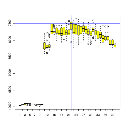
Figure 2: Boxplot representation (over 60 experiments) of ILvb for $Q\in\{1,\dots,40\}$. The maximum is reached at $Q_{IL_{vb}}=22$.

Thus, for $Q\in\{1,\dots,40\}$, we apply the methods of Hofman and Wiggins (2008) as well as our approach on this network. We compute the corresponding criteria and we repeat such procedure 60 times, for different initializations of $\boldsymbol{\tau}$. Indeed, to speed up the initialization, we first run a kmeans algorithm with $40$ classes and random initial centers. We then use the corresponding partitions as inputs of the hierarchical algorithm described in Section 3.2. The results for ILvb are presented as boxplots in Figure 2. The criterion finds its maximum for $Q_{ILvb}=22$ classes, while Daudin et al (2008) found $Q_{ICL}=21$. Thus, for this particular large data set, both ILvb and ICL lead to almost the same estimates of the number of latent classes.

Figure 3: Dot plot representation of the metabolic network after classification of the vertices into $Q_{VB}=22$ classes. The x-axis and y-axis correspond to the list of vertices in the network, from $1$ to $605$. Edges between pairs of vertices are represented by shaded dots.

We also compared the learnt partitions in the Bayesian and in the frequentist approach. Figure 3 is a dot plot representation of the metabolic network after having applied the Bayesian algorithm for $Q_{VB}=22$. Each vertex $i$ is classified into the class for which $\tau_{iq}$ is maximal (Maximum A Posteriori estimate). We observed very similar patterns in the frequentist approach. Among the classes, eight of them are cliques $\pi_{qq}=1$ and six have within probability connectivity greater than 0.5. As shown by Daudin et al (2008), these cliques or pseudo-cliques gather reactions involving a same compound. Thus, chorismate, pyruvate, L-aspartate, L-glutamate, D-glyceraldehyde-3-phosphate and ATP are all responsible for cliques. Moreover, as observed in Daudin et al (2008), since the connection probability between class 1 and 17 is 1, they correspond to a single clique which is associated to pyruvate. However that clique is split into two sub-cliques because of their different connectivities with reactions of classes 7 and 10. Since the approach of Hofman and Wiggins (2008) only looks for community structures, it can not retrieve such complex topologies, as shown in Section 5.1.2, and many classes such as class 1 and 17 were merged. We found $Q_{VBMOD}=14$.

6 Conclusion

In this paper, we showed how the Stochastic Block Model (SBM) could be described in a full Bayesian framework. We introduced some non informative conjugate priors over the model parameters and we described a variational Bayes EM algorithm which approximates the posterior distribution of all the latent variables and model parameters, given the observed data. Using this framework, we derived a non asymptotic model selection criterion, so-called ILvb, which approximates the marginal likelihood. By considering networks generated using SBM, we showed that ILvb focus on the estimation of the data density and provides a relevant estimation of the number of latent classes. We also illustrated the capacity of SBM to retrieve interesting structures in a large variety of networks, contrary to algorithms looking for community structures only. In future work, we will investigate approximate Bayesian computation methods for model selection. These simulation techniques seem particularly promising for the analysis of SBM where the likelihood of the observed data is intractable.

Appendix

Appendix A Approximation of $q(\operatorname{{\bf Z}}_{i})$ the conditional distribution of the latent variables

The optimal approximation at vertex $i$ is

$$q(\operatorname{{\bf Z}}_{i})=\mathcal{M}(\operatorname{{\bf Z}}_{i};\>1,\boldsymbol{\tau_{i}}=\{\tau_{i1},\dots,\tau_{iQ}\}),$$ (A.1)

where $\tau_{iq}$ is the probability (responsability) of node $i$ to belong to class $q$. It satisfies the relation

$$\tau_{iq}\propto e^{\psi(n_{q})-\psi(\sum_{l=1}^{Q}n_{l})}\prod_{j\neq i}^{N}\prod_{l=1}^{Q}e^{\tau_{jl}\Bigg{(}\psi(\zeta_{ql})-\psi(\eta_{ql}+\zeta_{ql})+X_{ij}\Big{(}\psi(\eta_{ql})-\psi(\zeta_{ql})\Big{)}\Bigg{)}},$$ (A.2)

where $\psi(.)$ is the digamma function. In order to optimize the distribution $q(\operatorname{{\bf Z}})$, we rely on a fixed point algorithm. Thus, given a matrix $\operatorname{\boldsymbol{\tau}}^{old}$, the algorithm builds a new matrix $\operatorname{\boldsymbol{\tau}}^{new}$ where each rows satisfies (A.2). After normalization, it then uses $\operatorname{\boldsymbol{\tau}}^{new}$ to build a new matrix and so on. The algorithm stops when $\sum_{i=1}^{N}\sum_{q=1}^{Q}|\tau_{iq}^{old}-\tau_{iq}^{new}|<eps$. In the experiment section, we set $eps=1e-6$.

Proof: According to variational Bayes, the optimal distribution $q(\operatorname{{\bf Z}}_{i})$ is given by

$$\ln q(\operatorname{{\bf Z}}_{i}) =\mbox{$\mathsf{E}$}_{\operatorname{{\bf Z}}^{\backslash i},\operatorname{\boldsymbol{\alpha}},\operatorname{\boldsymbol{\pi}}}[\ln p(\operatorname{{\bf X}},\operatorname{{\bf Z}},\operatorname{\boldsymbol{\alpha}},\operatorname{\boldsymbol{\pi}})]+\mathrm{cst}$$ (A.3)

$$=\mbox{$\mathsf{E}$}_{\operatorname{{\bf Z}}^{\backslash i},\operatorname{\boldsymbol{\pi}}}[\ln p(\operatorname{{\bf X}}|\operatorname{{\bf Z}},\boldsymbol{\pi)}]+\mbox{$\mathsf{E}$}_{\operatorname{{\bf Z}}^{\backslash i},\operatorname{\boldsymbol{\alpha}}}[\ln p(\operatorname{{\bf Z}}|\boldsymbol{\alpha)}]+\mathrm{cst}$$

$$=\mbox{$\mathsf{E}$}_{\operatorname{{\bf Z}}^{\backslash i},\operatorname{\boldsymbol{\pi}}}[\sum_{i^{{}^{\prime}}<j}\sum_{q,l}Z_{i^{\prime}q}Z_{jl}\Big{(}X_{i^{\prime}j}\ln\pi_{ql}+(1-X_{i^{\prime}j})\ln(1-\pi_{ql})\Big{)}]$$

$$\qquad\>\>\>\>\>+\mbox{$\mathsf{E}$}_{\operatorname{{\bf Z}}^{\backslash i},\operatorname{\boldsymbol{\alpha}}}[\sum_{i^{\prime}=1}^{N}\sum_{q=1}^{Q}Z_{i^{\prime}q}\ln\alpha_{q}]+\mathrm{cst}$$

$$=\sum_{q=1}^{Q}Z_{iq}\Bigg{(}\mbox{$\mathsf{E}$}_{\alpha_{q}}[\ln\alpha_{q}]+\sum_{j\neq i}^{N}\sum_{l=1}^{Q}\tau_{jl}\Big{(}X_{ij}\big{(}\mbox{$\mathsf{E}$}_{\pi_{ql}}[\ln\pi_{ql}]-\mbox{$\mathsf{E}$}_{\pi_{ql}}[\ln(1-\pi_{ql})]\big{)}$$

$$\qquad\>\>\>\>\>+\mbox{$\mathsf{E}$}_{\pi_{ql}}[\ln(1-\pi_{ql})]\Big{)}\Bigg{)}+\mathrm{cst}$$

$$=\sum_{q=1}^{Q}Z_{iq}\Bigg{(}\psi(n_{q})-\psi(\sum_{l=1}^{N}n_{l})+\sum_{j\neq i}^{N}\sum_{l=1}^{Q}\tau_{jl}\Big{(}X_{ij}\big{(}\psi(\eta_{ql})-\psi(\zeta_{ql})\big{)}$$

$$\qquad\>\>\>\>\>+\psi(\zeta_{ql})-\psi(\eta_{ql}+\zeta_{ql})\Big{)}\Bigg{)}+\mathrm{cst},$$

where $\operatorname{{\bf Z}}^{\backslash i}$ denotes the class of all nodes except node $i$. We have used $\mbox{$\mathsf{E}$}_{y}[\ln y]=\psi(a)-\psi(a+b)$ when $y\sim\operatorname{Beta}(y;\>a,b)$. Moreover, to simplify the calculations, the terms that do not depend on $\operatorname{{\bf Z}}_{i}$ have been absorbed into the constant. Taking the exponential of (A.3) and after normalization, we obtain the multinomial distribution (A.1).

Appendix B Optimization of $q(\operatorname{\boldsymbol{\alpha}})$.

The optimization of the lower bound with respect to $q(\operatorname{\boldsymbol{\alpha}})$ produces a distribution with the same functional form as the prior $p(\operatorname{\boldsymbol{\alpha}})$

$$q(\operatorname{\boldsymbol{\alpha}})=\operatorname{Dir}(\alpha;\>\mathbf{n}),$$ (B.1)

where

$$n_{q}=n_{q}^{0}+\sum_{i=1}^{N}\tau_{iq}.$$ (B.2)

Proof: According to variational Bayes, the optimal distribution $q(\operatorname{\boldsymbol{\alpha}})$ is given by

$$\ln q(\operatorname{\boldsymbol{\alpha}}) =\mbox{$\mathsf{E}$}_{\operatorname{{\bf Z}},\operatorname{\boldsymbol{\pi}}}[\ln p(\operatorname{{\bf X}},\operatorname{{\bf Z}},\operatorname{\boldsymbol{\alpha}},\operatorname{\boldsymbol{\pi}})]+\mathrm{cst}$$ (B.3)

$$=\mbox{$\mathsf{E}$}_{\operatorname{{\bf Z}}}[\ln p(\operatorname{{\bf Z}}|\operatorname{\boldsymbol{\alpha}})]+\ln p(\operatorname{\boldsymbol{\alpha}})+\mathrm{cst}$$

$$=\sum_{i=1}^{N}\sum_{q=1}^{Q}\tau_{iq}\ln\alpha_{q}+\sum_{q=1}^{Q}(n_{q}^{0}-1)\ln\alpha_{q}+\mathrm{cst}$$

$$=\sum_{q=1}^{Q}\left(n_{q}^{0}-1+\sum_{i=1}^{N}\tau_{iq}\right)\ln\alpha_{q}+\mathrm{cst}.$$

Taking the exponential of (B.3) and after normalization, we obtain the Dirichlet distribution (B.1).

Appendix C Optimization of $q(\operatorname{\boldsymbol{\pi}})$.

Again, the functional form of the prior $p(\operatorname{\boldsymbol{\pi}})$ is conserved through the variational optimization:

$$q(\operatorname{\boldsymbol{\pi}})=\prod_{q\leq l}^{Q}\operatorname{Beta}(\pi_{ql};\>\eta_{ql},\zeta_{ql}),$$ (C.1)

For $q\neq l$, the hyperparameter $\eta_{ql}$ is given by

$$\eta_{ql}=\eta_{ql}^{0}+\sum_{i\neq j}^{N}X_{ij}\tau_{iq}\tau_{jl},$$ (C.2)

and $\forall q$:

$$\eta_{qq}=\eta_{qq}^{0}+\sum_{i<j}^{N}X_{ij}\tau_{iq}\tau_{jq}.$$ (C.3)

Moreover, for $q\neq l$, the hyperparameter $\zeta_{ql}$ is given by

$$\zeta_{ql}=\zeta_{ql}^{0}+\sum_{i\neq j}^{N}(1-X_{ij})\tau_{iq}\tau_{jl},$$ (C.4)

and $\forall q$:

$$\zeta_{qq}=\zeta_{qq}^{0}+\sum_{i<j}^{N}(1-X_{ij})\tau_{iq}\tau_{jq}.$$ (C.5)

Proof : According to variational Bayes, the optimal distribution $q(\operatorname{\boldsymbol{\pi}})$ is given by

$$\ln q(\operatorname{\boldsymbol{\pi}}) =\mbox{$\mathsf{E}$}_{\operatorname{{\bf Z}},\operatorname{\boldsymbol{\alpha}}}[\ln p(\operatorname{{\bf X}},\operatorname{{\bf Z}},\operatorname{\boldsymbol{\alpha}},\operatorname{\boldsymbol{\pi}})]+\mathrm{cst}$$ (C.6)

$$=\mbox{$\mathsf{E}$}_{\operatorname{{\bf Z}}}[\ln p(\operatorname{{\bf X}}|\operatorname{{\bf Z}},\operatorname{\boldsymbol{\pi}})]+\ln p(\operatorname{\boldsymbol{\pi}})+\mathrm{cst}$$

$$=\sum_{i<j}^{N}\sum_{q,l}^{Q}\tau_{iq}\tau_{jl}\Big{(}X_{ij}\ln\pi_{ql}+(1-X_{ij})\ln(1-\pi_{ql})\Big{)}$$

$$\qquad\>\>\>\>\>+\sum_{q\leq l}^{Q}\Big{(}(\eta_{ql}^{0}-1)\ln\pi_{ql}+(\zeta_{ql}^{0}-1)\ln(1-\pi_{ql})\Big{)}+\mathrm{cst}$$

$$=\sum_{q<l}^{Q}\sum_{i\neq j}^{N}\tau_{iq}\tau_{jl}\Big{(}X_{ij}\ln\pi_{ql}+(1-X_{ij})\ln(1-\pi_{ql})\Big{)}$$

$$\qquad\>\>\>\>\>+\sum_{q=1}^{Q}\sum_{i<j}^{N}\tau_{iq}\tau_{jq}\Big{(}X_{ij}\ln\pi_{qq}+(1-X_{ij})\ln(1-\pi_{qq})\Big{)}$$

$$\qquad\>\>\>\>\>+\sum_{q\leq l}^{Q}\Big{(}(\eta_{ql}^{0}-1)\ln\pi_{ql}+(\zeta_{ql}^{0}-1)\ln(1-\pi_{ql})\Big{)}+\mathrm{cst}$$

$$=\sum_{q<l}^{Q}\Bigg{(}\Big{(}\eta_{ql}^{0}-1+\sum_{i\neq j}^{N}\tau_{iq}\tau_{jl}X_{ij}\Big{)}\ln\pi_{ql}+\Big{(}\zeta_{ql}^{0}-1+\sum_{i\neq j}^{N}\tau_{iq}\tau_{jl}(1-X_{ij})\Big{)}\ln(1-\pi_{ql})\Bigg{)}$$

$$\qquad\>\>\>\>\>+\sum_{q=1}^{Q}\Bigg{(}\Big{(}\eta_{qq}^{0}-1+\sum_{i<j}^{N}\tau_{iq}\tau_{jq}X_{ij}\Big{)}\ln\pi_{qq}+\Big{(}\zeta_{qq}^{0}-1+\sum_{i<j}^{N}\tau_{iq}\tau_{jq}(1-X_{ij})\Big{)}\ln(1-\pi_{qq})\Bigg{)}.$$

Taking the exponential of (C.6) and after normalization, we obtain the product of $\operatorname{Beta}$ distribution (C.1).

Appendix D Lower bound.

The lower bound takes a simple form after the variational Bayes M-step. Indeed, it only depends on the posterior probabilities $\tau_{iq}$ as well as the normalizing constants of the Dirichlet and Beta distributions

$$\mathcal{L}\Big{(}q(.)\Big{)}=\ln\{\frac{\Gamma(\sum_{q=1}^{Q}n_{q}^{0})\prod_{q=1}^{Q}\Gamma(n_{q})}{\Gamma(\sum_{q=1}^{Q}n_{q})\prod_{q=1}^{Q}\Gamma(n_{q}^{0})}\}+\sum_{q\leq l}^{Q}\ln\{\frac{\Gamma(\eta_{ql}^{0}+\zeta_{ql}^{0})\Gamma(\eta_{ql})\Gamma(\zeta_{ql})}{\Gamma(\eta_{ql}+\zeta_{ql})\Gamma(\eta_{ql}^{0})\Gamma(\zeta_{ql}^{0})}\}-\sum_{i=1}^{N}\sum_{q=1}^{Q}\tau_{iq}\ln\tau_{iq}.$$ (D.1)

Proof : The lower bound is given by

$$\mathcal{L}\Big{(}q(.)\Big{)} =\sum_{\operatorname{{\bf Z}}}\int\int q(\operatorname{{\bf Z}},\operatorname{\boldsymbol{\alpha}},\operatorname{\boldsymbol{\pi}})\ln\{\frac{p(\operatorname{{\bf X}},\operatorname{{\bf Z}},\operatorname{\boldsymbol{\alpha}},\operatorname{\boldsymbol{\pi}})}{q(\operatorname{{\bf Z}},\operatorname{\boldsymbol{\alpha}},\operatorname{\boldsymbol{\pi}})}\}d\alpha d\pi$$ (D.2)

$$=\mbox{$\mathsf{E}$}_{\operatorname{{\bf Z}},\operatorname{\boldsymbol{\alpha}},\operatorname{\boldsymbol{\pi}}}[\ln p(\operatorname{{\bf X}},\operatorname{{\bf Z}},\operatorname{\boldsymbol{\alpha}},\operatorname{\boldsymbol{\pi}})]-\mbox{$\mathsf{E}$}_{\operatorname{{\bf Z}},\operatorname{\boldsymbol{\alpha}},\operatorname{\boldsymbol{\pi}}}[\ln q(\operatorname{{\bf Z}},\operatorname{\boldsymbol{\alpha}},\operatorname{\boldsymbol{\pi}})]$$

$$=\mbox{$\mathsf{E}$}_{\operatorname{{\bf Z}},\operatorname{\boldsymbol{\pi}}}[\ln p(\operatorname{{\bf X}}|\operatorname{{\bf Z}},\operatorname{\boldsymbol{\pi}})]+\mbox{$\mathsf{E}$}_{\operatorname{{\bf Z}},\operatorname{\boldsymbol{\alpha}}}[\ln p(\operatorname{{\bf Z}}|\operatorname{\boldsymbol{\alpha}})]+\mbox{$\mathsf{E}$}_{\operatorname{\boldsymbol{\alpha}}}[\ln p(\operatorname{\boldsymbol{\alpha}})]+\mbox{$\mathsf{E}$}_{\operatorname{\boldsymbol{\pi}}}[\ln p(\operatorname{\boldsymbol{\pi}})]$$

$$\qquad\>\>\>\>\>-\sum_{i=1}^{N}\mbox{$\mathsf{E}$}_{\operatorname{{\bf Z}}_{i}}[\ln q(\operatorname{{\bf Z}}_{i})]-\mbox{$\mathsf{E}$}_{\operatorname{\boldsymbol{\alpha}}}[\ln q(\operatorname{\boldsymbol{\alpha}})]-\mbox{$\mathsf{E}$}_{\operatorname{\boldsymbol{\pi}}}[\ln q(\boldsymbol{\pi)}]$$

$$=\sum_{i<j}^{N}\sum_{q,l}^{Q}\tau_{iq}\tau_{jl}\Bigg{(}X_{ij}\Big{(}\psi(\eta_{ql})-\psi(\zeta_{ql})\Big{)}+\psi(\zeta_{ql})-\psi(\eta_{ql}+\zeta_{ql})\Bigg{)}$$

$$\qquad\>\>\>\>\>+\sum_{i=1}^{N}\sum_{q=1}^{Q}\tau_{iq}\Big{(}\psi(n_{q})-\psi(\sum_{l=1}^{Q}n_{l})\Big{)}+\ln\Gamma(\sum_{q=1}^{Q}n_{q}^{0})-\sum_{q=1}^{Q}\ln\Gamma(n_{q}^{0})$$

$$\qquad\>\>\>\>\>+\sum_{q=1}^{Q}\Big{(}n_{q}^{0}-1\Big{)}\Big{(}\psi(n_{q})-\psi(\sum_{l=1}^{Q}n_{l})\Big{)}+\sum_{q\leq l}^{Q}\Bigg{(}\ln\Gamma(\eta_{ql}^{0}+\zeta_{ql}^{0})$$

$$\qquad\>\>\>\>\>-\ln\Gamma(\eta_{ql}^{0})-\ln\Gamma(\zeta_{ql}^{0})+(\eta_{ql}^{0}-1)\Big{(}\psi(\eta_{ql})-\psi(\eta_{ql}+\zeta_{ql})\Big{)}$$

$$\qquad\>\>\>\>\>+(\zeta_{ql}^{0}-1)\Big{(}\psi(\zeta_{ql})-\psi(\eta_{ql}+\zeta_{ql})\Big{)}\Bigg{)}-\sum_{i=1}^{N}\sum_{q=1}^{Q}\tau_{iq}\ln\tau_{iq}$$

$$\qquad\>\>\>\>\>-\ln\Gamma(\sum_{q=1}^{Q}n_{q})+\sum_{q=1}^{Q}\ln\Gamma(n_{q})-\sum_{q=1}^{Q}\Big{(}n_{q}-1\Big{)}\Big{(}\psi(n_{q})-\psi(\sum_{l=1}^{Q}n_{l})\Big{)}$$

$$\qquad\>\>\>\>\>-\sum_{q\leq l}^{Q}\Bigg{(}\ln\Gamma(\eta_{ql}+\zeta_{ql})-\ln\Gamma(\eta_{ql})-\ln\Gamma(\zeta_{ql})$$

$$\qquad\>\>\>\>\>+(\eta_{ql}-1)\Big{(}\psi(\eta_{ql})-\psi(\eta_{ql}+\zeta_{ql})\Big{)}+(\zeta_{ql}-1)\Big{(}\psi(\zeta_{ql})-\psi(\eta_{ql}+\zeta_{ql})\Big{)}\Bigg{)}.$$

Therefore

$$\mathcal{L}\Big{(}q(.)\Big{)} =\sum_{q<l}^{Q}\Bigg{(}\Big{(}\eta_{ql}^{0}-\eta_{ql}+\sum_{i\neq j}^{N}\tau_{iq}\tau_{jl}X_{ij}\Big{)}\Big{(}\psi(\eta_{ql})-\psi(\eta_{ql}+\zeta_{ql})\Big{)}$$ (D.3)

$$\qquad\>\>\>\>\>+\Big{(}\zeta_{ql}^{0}-\zeta_{ql}+\sum_{i\neq j}^{N}\tau_{iq}\tau_{jl}(1-X_{ij})\Big{)}\Big{(}\psi(\zeta_{ql})-\psi(\eta_{ql}+\zeta_{ql})\Big{)}\Bigg{)}$$

$$\qquad\>\>\>\>\>+\sum_{q=1}^{Q}\Bigg{(}\Big{(}\eta_{qq}^{0}-\eta_{qq}+\sum_{i<j}^{N}\tau_{iq}\tau_{jq}X_{ij}\Big{)}\Big{(}\psi(\eta_{qq})-\psi(\eta_{qq}+\zeta_{qq})\Big{)}$$

$$\qquad\>\>\>\>\>+\Big{(}\zeta_{qq}^{0}-\zeta_{qq}+\sum_{i<j}^{N}\tau_{iq}\tau_{jq}(1-X_{ij})\Big{)}\Big{(}\psi(\zeta_{qq})-\psi(\eta_{qq}+\zeta_{qq})\Big{)}\Bigg{)}$$

$$\qquad\>\>\>\>\>+\sum_{q=1}^{Q}\Big{(}n_{q}^{0}-n_{q}+\sum_{i=1}^{N}\tau_{iq}\Big{)}\Big{(}\psi(n_{q})-\psi(\sum_{l=1}^{Q}n_{l})\Big{)}$$

$$\qquad\>\>\>\>\>+\ln\{\frac{\Gamma(\sum_{q=1}^{Q}n_{q}^{0})\prod_{q=1}^{Q}\Gamma(n_{q})}{\Gamma(\sum_{q=1}^{Q}n_{q})\prod_{q=1}^{Q}\Gamma(n_{q}^{0})}\}+\sum_{q\leq l}^{Q}\ln\{\frac{\Gamma(\eta_{ql}^{0}+\zeta_{ql}^{0})\Gamma({\eta_{ql}})\Gamma(\zeta_{ql})}{\Gamma(\eta_{ql})+\zeta_{ql}\Gamma(\eta_{ql}^{0})\Gamma(\zeta_{ql}^{0})}\}$$

$$\qquad\>\>\>\>\>-\sum_{i=1}^{N}\sum_{q=1}^{Q}\tau_{iq}\ln\tau_{iq}.$$

After the variational Bayes M-step, most of the terms in the lower bound vanish since

• $\forall q\>:n_{q}=n_{q}^{0}+\sum_{i=1}^{N}\tau_{iq}$.

• $\forall q\neq l\>:\eta_{ql}=\eta_{ql}^{0}+\sum_{i\neq j}^{N}X_{ij}\tau_{iq}\tau_{jl}$,

• $\forall q\>:\eta_{qq}=\eta_{qq}^{0}+\sum_{i<j}^{N}X_{ij}\tau_{iq}\tau_{jq}$.

• $\forall q\neq l\>:\zeta_{ql}=\zeta_{ql}^{0}+\sum_{i\neq j}^{N}(1-X_{ij})\tau_{iq}\tau_{jl}$,

• $\forall q\>:\zeta_{qq}=\zeta_{qq}^{0}+\sum_{i<j}^{N}(1-X_{ij})\tau_{iq}\tau_{jq}$.

Only the terms depending on the probabilities $\tau_{iq}$ and the normalizing constants of the Dirichlet and Beta distributions remain.

References

- Airoldi et al (2008) Airoldi E, Blei D, Fienberg S, Xing E (2008) Mixed-membership stochastic blockmodels. Journal of Machine Learning Research 9:1981–2014
- Albert and Barabási (2002) Albert R, Barabási A (2002) Statistical mechanics of complex networks. Modern Physics 74:47–97
- Allman et al (2009) Allman E, Matias C, Rhodes J (2009) Identifiability of parameters in latent structure models with many observed variables. Annals of Statistics 37(6A):3099–3132, URL http://www.imstat.org/aos/
- Attias (1999) Attias H (1999) Inferring parameters and structure of latent variable models by variational bayes. In: Laskey K, Prade H (eds) Uncertainty in Artificial Intelligence : proceedings of the fifth conference, Morgan Kaufmann, pp 21–30
- Barabási and Oltvai (2004) Barabási A, Oltvai Z (2004) Network biology: understanding the cell’s functional organization. Nature Rev Genet 5:101–113
- Biernacki et al (2000) Biernacki C, Celeux G, Govaert G (2000) Assessing a mixture model for clustering with the integrated completed likelihood. IEEE Trans Pattern Anal Machine Intel 7:719–725
- Biernacki et al (2010) Biernacki C, Celeux G, Govaert G (2010) Exact and monte carlo calculations of integrated likelihoods for the latent class model. Journal of Statistical Planning and Inference 140:2991–3002
- Boer et al (2006) Boer P, Huisman M, Snijders T, Steglich C, Wichers L, Zeggelink E (2006) StOCNET : an open software system for the advanced statistical analysis of social networks. Groningnen:ProGAMMA/ICS, version 1.7
- Burnham and Anderson (2004) Burnham K, Anderson D (2004) Model selection and multi-model inference: a practical information-theoric approach. Springer-Verlag
- Corduneanu and Bishop (2001) Corduneanu A, Bishop C (2001) Variational bayesian model selection for mixture distributions. In: Richardson T, Jaakkola T (eds) Artificial Intelligence and Statistics : proceedings of the eighth conference, Morgan Kaufmann, pp 27–34
- Danon et al (2005) Danon L, Diaz-Guilera A, Duch J, Arenas A (2005) Comparing community structure identification. J Stat Mech
- Daudin et al (2008) Daudin J, Picard F, Robin S (2008) A mixture model for random graph. Statistics and Computing 18:1–36
- Dempster et al (1977) Dempster A, Laird N, Rubin DB (1977) Maximum likelihood for incomplete data via the em algorithm. Journal of the Royal Statistical Society B39:1–38
- Estrada and Rodriguez-Velazquez (2005) Estrada E, Rodriguez-Velazquez JA (2005) Spectral measures of bipartivity in complex networks. Phys Rev E 72
- Fienberg and Wasserman (1981) Fienberg S, Wasserman S (1981) Categorical data analysis of single sociometric relations. Sociological Methodology 12:156–192
- Frank and Harary (1982) Frank O, Harary F (1982) Cluster inference by using transitivity indices in empirical graphs. Journal of the American Statistical Association 77:835–840
- Girvan and Newman (2002) Girvan M, Newman MEJ (2002) Community structure in social and biological networks. Proc Natl Acad Sci 99:7821–7826
- Handcock et al (2007) Handcock MS, Raftery AE, Tantrum JM (2007) Model-based clustering for social networks. Journal of the Royal Statistical Society, Series A 170:1–22
- Hathaway (1986) Hathaway R (1986) Another interpretation of the em algorithm for mixture distributions. Statistics & Probability Letters 4:53–56
- Hoff et al (2002) Hoff PD, Raftery AE, Handcock MS (2002) Latent space approaches to social network analysis. Journal of the Royal Statistical Society 97:1090–1098
- Hofman and Wiggins (2008) Hofman J, Wiggins C (2008) A bayesian approach to network modularity. Physical Review Letters 100
- Holland et al (1983) Holland P, Laskey K, Leinhardt S (1983) Stochastic blockmodels: some first steps. Social networks 5:109–137
- Jeffreys (1946) Jeffreys H (1946) An invariant form for the prior probability in estimations problems. In: Proceedings of the Royal Society of London. Series A, vol 186, pp 453–461
- Kemp et al (2004) Kemp C, Griffiths T, Tenenbaum J (2004) Discovering latent classes in relational data. Tech. rep., MIT
- Krivitsky and Handcock (2009) Krivitsky P, Handcock M (2009) The latentnet package. Statnet project, version 2.1-1
- Lacroix et al (2006) Lacroix V, Fernandes C, Sagot MF (2006) Motif search in graphs: Application to metabolic networks. Transactions in Computational Biology and Bioinformatics 3:360–368
- Mariadassou et al (2010) Mariadassou M, Robin S, Vacher C (2010) Uncovering latent structure in valued graphs: a variational approach. Annals of Applied Statistics 4(2)
- McLachlan and Krishnan (1997) McLachlan G, Krishnan T (1997) The EM algorithm and extensions. New York: John Wiley
- Neal and Hinton (1998) Neal R, Hinton G (1998) A view of the EM algorithm that justifies incremental, sparse, and other variants. In: Jordan MI (ed) Learning in Graphical Models, Kluwer, Dordrecht
- Newman and Leicht (2007) Newman M, Leicht E (2007) Mixture models and exploratory analysis in networks. PNAS 104:9564–9569
- Nowicki and Snijders (2001) Nowicki K, Snijders T (2001) Estimation and prediction for stochastic blockstructures. Journal of the American Statistical Association 96:1077–1087
- Palla et al (2007) Palla G, Barabási AL, Vicsek T (2007) Quantifying social group evolution. Nature 446:664–667
- Snijders and Nowicki (1997) Snijders T, Nowicki K (1997) Estimation and prediction for stochastic block-structures for graphs with latent block structure. Journal of Classification 14:75–100
- Svensén and Bishop (2004) Svensén M, Bishop C (2004) Robust bayesian mixture modelling. Neurocomputing 64:235–252
- Watts and Strogatz (1998) Watts DJ, Strogatz SH (1998) Collective dynamics of small-world networks. Nature 393:440–442
- White et al (1976) White H, Boorman S, Breiger R (1976) Social structure from multiple networks. i. blockmodels of roles and positions. American Journal of Sociology 81:730–780
- Zanghi et al (2008) Zanghi H, Ambroise C, Miele V (2008) Fast online graph clustering via erdös renyi mixture. Pattern Recognition 41(12):3592–3599