Screening masses in quenched $\left(2+1\right)d$ Yang-Mills theory: universality from dynamics?

Abstract

We compute the spectrum of gluonic screening-masses in the $0^{++}$ channel of quenched 3d Yang-Mills theory near the phase-transition. Our finite-temperature lattice simulations are performed at scaling region, using state-of-art techniques for thermalization and spectroscopy, which allows for thorough data extrapolations to thermodynamic limit. Ratios among mass-excitations with the same quantum numbers on the gauge theory, 2d Ising and $\lambda\phi^{4}$ models are compared, resulting in a nice agreement with predictions from universality. In addition, a gauge-to-scalar mapping, previously employed to fit QCD Green’s functions at deep IR, is verified to dynamically describe these universal spectroscopic patterns.

1 Introduction

The lattice formulation of gauge theories [1] as QCD allows for ab initio systematically well-controlled numerical investigations of most theoretical key aspects, like confinement and chiral symmetry breaking [2], at non-perturbative regime. For instance, at high temperatures or densities when deconfinement phase-transition takes place in non-abelian gauge theories, Monte Carlo simulations have been essential to unveil how matter behaves under extreme thermodynamical conditions [3].

Hence, quantum field theories (QFT) on the lattice can be understood as classical models of statistical mechanics. Some enlightening interconnections usually appear from finite temperature studies [4], as in the case of a long-standing conjecture — designed upon general symmetry arguments — from Svetistky and Jaffe [5] relating universal properties from finite-temperature $SU(N)$ gauge-theories in $\left(d+1\right)$ dimensions to $d-$dimensional $Z_{N}-$spin systems at criticality. This has been corroborated by computations of critical (static and dynamic) exponents, universal amplitudes, and correlation functions: see for example, respectively [6][7][8].

Still, under the spontaneous breaking of global $Z_{N}$ center-symmetry, $SU(N)$ gauge theories were shown — in 4-dimensions and $N\leq 3$ — to exhibit a rich spectrum of gluonic screening-masses, whose ratios among equivalent excitations are shared by $Z_{N}-$spin systems [9, 10]. Despite the effectiveness of universality-based reasoning, investigations on symplectic gauge theories compel for a still elusive dynamical description of deconfinement [11], instead of relying completely on $Z_{N}-$invariance as a physical fingerprint.

New perspectives have appeared over the last years, such as a unified picture of confinement emerging from various analysis of Green´s functions of non-abelian gauge theories [2, 12, 13, 14, 15]. While analytical (decoupling) solutions of Dyson-Schwinger equations [12, 13] and gauge-to-scalar mappings [15] predict non-vanishing gluon propagators at deep infrared for $d>2$, lattice computations provide evidences of gluons having dynamically-generated masses [14].

These features stay unchanged at finite-temperatures, which supports a strongly-coupled plasma at the vicinity of phase-transition, thus agreeing with dimensional-reduced theories [16] and (universal) results from AdS/QCD correspondence [17]. Additionally, properties derived from gauge-dependent gluon propagators would also be compared with spectroscopical analysis employing gauge-invariant correlators [18] (free from Gribov ambiguities [19]), which may deepen physical insights into QFT- thermodynamics. For a more comprehensive review on gluonic bound-states using methods from spectroscopy, at zero and finite-temperatures, see also [20].

In this article, we investigate through Monte Carlo simulations the gluonic screening-spectrum of quenched three-dimensional Yang-Mills (YM) theory on the lattice. State-of-art techniques for spectroscopy, such as the variational-method [21] and recursively-smeared interpolators [9, 10], are employed to compute excitations on the $0^{++}$ channel. Using an improved thermalization algorithm [22] we carry out simulations at asymptotic region with ameliorated critical-slowing-down (CSD) [23], UV-discretization and IR-cutoff effects [24]. We compare mass-ratios of YM theory and exactly-solvable bidimensional systems in the same universality-class (i.e. the Ising and $\lambda\phi^{4}$ models) [5], therefore enabling us to check predictions from universality [5, 9, 10] and other dynamical mechanisms [11, 15].

This work is organized as follows: in section II there is a review of the major aspects of universality and its implications for thermal excitations on gauge theories and spin-systems at the vicinity of critical points. Section III outlines the general simulation setup, as well as the modified heat-bath algorithm used for ensuring more efficient thermalization of gauge fields. Spectroscopical techniques for extracting screening masses are the topic of Section IV. Section V presents numerical results and comparative data analysis. Conclusions of the present work and its outlook are discussed in Section VI.

2 Universality: field theories and spin-systems

The finite-temperature formalism for $d-$dimensional gauge theories on the lattice [1, 4] uses an asymmetric euclidean spacetime, whose physical volume $V=a^{d}\cdot L_{S}^{d-1}\cdot L_{T}$ has $L_{S}$ and $L_{T}$ as spatial and temporal (adimensional) lattice sides, respectively. Thus, under the assumption $a\ll\left(a\cdot L_{T}\right)<\left(a\cdot L_{S}\right)$, where $a$ is the (dimensionful) lattice spacing, one can set the temperature of physical equilibrium as $T{}^{-1}=a\cdot L_{T}$. As a consequence of the formalism, in the vicinity of phase transitions, arguments from universality [5] state that finite-temperature QFTs for $SU(N)$ gauge groups in $\left(d+1\right)$ dimensions belong to the same universality class of globally $Z_{N}$-invariant spin-systems in $d$ dimensions.

For the particular case of $SU(N=2)$ gauge theory, a second-order (i.e. critical) deconfinement phase-transition is expected. This theory can be implemented on the lattice by the Wilson action

$$S_{W}\left[U\right]\equiv\beta\sum_{x}\sum_{\mu,\nu=1}^{d}\left\{1-\frac{1}{2}Re(TrP_{\mu\nu})\right\},$$ (1)

using $SU(2)$ gauge-links $U_{\mu}\left(x\right)$ and the plaquette

$$P_{\mu\nu}\equiv U_{\mu}\left(x\right)U_{\nu}\left(x+\hat{\mu}a\right)U_{\mu}^{-1}\left(x+\hat{\nu}a\right)U_{\nu}^{-1}\left(x\right),$$ (2)

with lattice-coupling $\beta=2N/g_{s}^{2}a^{4-d}$ and gauge-field coupling constant $g_{s}^{2}$. The action Eq.(1) is invariant under transformations generated by center-elements of the gauge-group, hence, spatial loops — in contradistinction to temporal ones — are insensitive to temperature-induced symmetry breaking. Then, a natural order parameter is given by a temporal loop, the so called Polyakov loop $\bar{L}\equiv\left\langle L\left(x,y,z\right)\right\rangle=\left\langle Tr\prod_{n=1}^{n=L_{T}}U_{T}\left(x,y,z,an\right)\right\rangle$ [25], which measures the potential energy necessary to free a quark [3].

On the other hand, the $3d$ Ising model is a well-known spin-system that undergoes a second-order phase-transition, for $\beta_{I}=\beta_{critical}$, due to a global $Z_{2}-$symmetry breaking universally related to the finite-temperature $(3+1)d$ YM theory. It is described by the action

$$S_{I}=-\beta_{I}\sum_{<n,m>}s_{n}s_{m}.$$ (3)

In this same universality class is the $3d$ lattice-regularized $\phi^{4}$ theory, whose action is

$$S_{\phi}=-\beta_{\phi}\sum_{<n,m>}\phi{}_{n}\phi_{m}+\sum_{n}\phi{}_{n}^{2}+\lambda\sum_{n}\left(\phi{}_{n}^{2}-1\right)^{2}.$$ (4)

In both cases, the order parameters are expectation values of fundamental fields, e.g. the magnetization $(\bar{m)}$ or the v.e.v. $\left(\bar{\phi}\right)$ of the scalar-field, which behaves as the Polyakov loop $\left(\bar{L}\right)$ in the YM theory [9].

The analogy among order-parameters $\bar{m},\bar{\phi}$ and $\bar{L}$ can also be extended to their correlation functions. The connected correlation function $G_{C}$ is usually expressed as

$$\begin{array}[]{c}G\left(\left|r_{2}-r_{1}\right|\right)_{C}\equiv<O\left(r_{2}\right)O^{\dagger}\left(r_{1}\right)>-<O\left(r_{2}\right)><O^{\dagger}\left(r_{1}\right)>=\\ \underset{i}{\sum}A_{i}\left(e^{-m_{i}\left|r_{2}-r_{1}\right|}+e^{-m_{i}\left(L_{S}-\left|r_{2}-r_{1}\right|\right)}\right),\end{array}$$ (5)

which is a sum over each mass $\left(m_{i}\right)$ of the spectrum of the operator $O$, in an $L_{S}-$periodic lattice. Thus, when $O=m,$ one gets excitations from a magnetic system or, with $O=L$, the spectrum of screening-masses for the gluonic field is recovered. While in the first case the spectrum is generated by a magnetic phase-transition that breaks the global $Z_{2}-$symmetry, in the latter case it is due to a spontaneous $Z_{2}$-center symmetry breaking of the $SU(2)$ gauge group [5, 9, 10].

Although inherently different in nature, the aforementioned phase-transitions constitute critical phenomena in the same universality class [4]. Thus, one may expect that universality [5] can predict some dynamical aspects of gauge theories, such as mass-ratios [26] of excitations in Eq.(5), to be shared with statistical-mechanical systems. While evidences supporting this hypothesis are accumulating [9, 10], arguments entirely based on universality are not enough to describe deconfinement in sympletic (or exceptional) gauge theories [11]. Thus, a broader dynamical picture may be needed [15].

An improved understanding of such dynamics may be obtained by comparing the spectrum of gauge theories and exactly-solvable systems in the same universality class. For instance, the $2d$ Ising model is well-described by a free-fermion field theory near criticality, whose spectrum of excitations — for $n$ integer — turns to be

$$M_{n}=nM_{0},$$ (6)

where $M_{0}$ is a mass-gap proportional to $|\tau|$: the deviation from critical temperature [27]. At the same time, the spectrum of $\lambda\phi^{4}$ theory is analytically calculated by a gradient-expansion [28], which results with mass-scales $(\Lambda_{broken})$ — and integer $k$ — for the broken phase

$$M_{k}=k\Lambda_{broken}.$$ (7)

Therefore, one can apply Monte Carlo methods to exploit whether the screening spectrum of the YM theory matches expectations from Eq.(6) and Eq.(7) near criticality, a regime where correspondences are expected, but other non-perturbative techniques are less effective (since the theory is dynamically trivial just in 2d; i.e., at the $T\rightarrow\infty$ limit [29, 30]).

3 Algorithms

Since in the vicinities of phase-transitions the CSD phenomena [23] afflicts the generation of statistically independent gauge-configurations more severely, continuous efforts toward the improvement of thermalization algorithms are ubiquitous for Monte Carlo simulations. To ensure an efficient thermalization of gluonic fields, we applied our modified heat bath algorithm (MHB), which was shown to be faster [22] than the usual heat bath (HB) algorithm [31, 32].

Usually, when an $SU(2)$ lattice-gauge theory is considered [22], one can factorize the action Eq.(1) as a sum over many single-link actions $S_{1-link}$ as

$$S_{1-link}=-\frac{\beta}{2}Tr\left[U_{\mu}\left(x\right)H_{\mu}\left(x\right)\right],$$ (8)

with $U_{\mu}\left(x\right)\in SU\left(2\right);$ $H_{\mu}\left(x\right)=N_{\mu}\left(x\right)\tilde{H_{\mu}}\left(x\right)$ is a sum over staples — i.e., it is proportional to an SU(2) matrix — where $\tilde{H_{\mu}}\left(x\right)\in SU\left(2\right)$ and $N_{\mu}\left(x\right)=\sqrt{\det H_{\mu}\left(x\right)}$.

Then, by using Eq.(8) and the invariance of the group measure under group multiplication [31], the usual HB update is obtained

$$U_{\mu}^{old}\left(x\right)\longrightarrow U_{\mu}^{new}\left(x\right)=V\tilde{H_{\mu}^{\dagger}}\left(x\right),$$ (9)

where $V=v_{0}I+i\vec{\cdot v}\cdot\vec{\sigma}\in SU\left(2\right)$ is randomly generated by choosing $v_{0}$ distributed as $\sqrt{1-v_{0}\mathchoice{\hbox{{\texttwosuperior}}}{\hbox{{\texttwosuperior}}}{\hbox{{\texttwosuperior}}}{\hbox{{\texttwosuperior}}}}$$\exp\left(\beta Nv_{0}\right)dv_{0}$ and $\vec{v}$ is randomly chosen in $\mathbb{R}^{3}$. Our algorithm [22] proceeds as the HB algorithm to generate the updating matrix $V$, except for the additional step

• Transform the new vector-components of V as $\vec{v}\rightarrow-sgn(\vec{v}\cdot\vec{w})\vec{v}$,

where $W=w_{0}I+i\cdot\vec{w}\cdot\vec{\sigma}=U_{\mu}^{old}\left(x\right)\tilde{H_{\mu}}\left(x\right)$, and $sgn$ is the sign function.

Still, MHB may be seen as a modification of the overheat-bath algorithm (OH) [33] that incorporates a micro-canonical move [34] into a heat-bath step. However, while in MHB all components of the vector $\vec{v}$ are randomly generated (i.e., except for its sign) in very close similarity to HB, the OH algorithm deterministically sets $\vec{v}=-\vec{w}$ (and renormalizes it as $\left\|\vec{v}\right\|=\sqrt{1-v_{0}^{2}}$). Thus, OH incorporates a microcanonical move in an exact, but maybe non-ergodic (see for example discussions in [22]) algorithm, which is corrected — by construction — in the MHB version.

4 Spectroscopical methods

The spectrum of excitations of a field theory on the lattice can be directly extracted by brute-force least-squares fitting from Eq.(5) using a multiple-exponential decay function. Despite being straightforward, this method has several drawbacks and allows for reliable results just when high-quality statistics is available. More robust techniques such as Bayesian fit [35] or the Evolutionary fitting [36] would constitute alternatives to overcoming these difficulties. However, here we use another state-of-art approach, namely the variational method [21], broadly employed in hadron spectroscopy [37].

On the variational method a proper set of base-operators (i.e., the interpolators $O_{i}$) has to be chosen for building a cross-correlation matrix

$$C_{ij}\left(\left|r\right|\right)\equiv<O_{i}\left(r\right)O_{j}^{\dagger}\left(0\right)>-<O_{i}\left(r\right)><O_{j}^{\dagger}\left(0\right)>,$$ (10)

which may be diagonalized in a generalized eigenvalue problem (properly normalized at some $r_{0}<L_{S}$), resulting in

$$C\left(r\right)\cdot\vec{v_{n}}=\lambda_{n}\left(r,r_{0}\right)\cdot C\left(r_{0}\right)\cdot\vec{v_{n}},$$ (11)

where eigenvalues behave as

$$\lambda_{n}\left(r,r_{0}\right)\varpropto e^{-\left(r-r_{0}\right)m_{n}}\left[1+\mathcal{O}\left(e^{-\left(r-r_{0}\right)\Delta m_{n}}\right)\right].$$ (12)

Generally, $\Delta m_{n}$ is the mass difference to the closest lying state, where each interpolator $O_{i}$ (projected to defined momentum-states) has quantum numbers in a given channel.

Within a large enough basis of independent interpolators, each eigenvalue of Eq.(10) will decay as the leading order of Eq.(12). Thus, the slowest decay-mode of eigenvalues is associated with the ground state, while the fastest one gives the highest-excitated state. This implies that simple fits of a few parameters may be nicely done, since single-exponentials dominate the signal in the whole range. In order to identify proper fit-ranges, it is useful to locate stable plateaus not only for effective-masses of $\lambda_{n}$

$$m_{n}^{eff}\left(r+1/2\right)=\ln\left(\frac{\lambda_{n}\left(r\right)}{\lambda_{n}\left(r+1\right)}\right),$$ (13)

but also in their associated eigenvectors $\vec{v_{k},}$ which work as fingerprints of each state.

We are interested in a set of interpolators that generates scalar screening-excitations in the $0^{++}$ channel. An efficient method for building this is to apply recursive smearing-steps over usual wall-averaged (i.e. zero-momentum) Polyakov loop operator [9], which is defined by

$$\overline{L}\left(x\right)=\frac{1}{\left(L_{S}\right)_{y}}\sum_{n=1}^{n=\left(L_{S}\right)_{y}}L\left(x,na\right).$$ (14)

It enables access to all length-scales on the lattice through the computation of cross-correlation functions among nth-smeared interpolators (i.e. $P^{\left(n\right)}$), which are constructed iteractively (for increasing smearing steps $n$) from the usual Polyakov loop ($\overline{L}\left(x\right)$) . That operators are assembled following the rule

$$\begin{array}[]{c}P^{(0)}\left(x\right)=\overline{L}\left(x\right)\\ P^{(n+1)}\left(x\right)=sign\left(u\right)\left[\left(1-\omega\right)\left|u\right|+\omega\left\langle P^{(n)}\right\rangle\right]\\ u=\frac{1}{2}\left[P^{(n)}\left(y-a\right)+P^{(n)}\left(y+a\right)\right],\end{array}$$ (15)

where $\omega\in\left(0,1\right]$ and we have taken $\omega=0.1$.

In addition, a compromise between signal-to-noise and maximal linear independence of correlators must be attained [38], which is achieved by looking for a set of interpolators that minimizes the conditioning number ($\kappa$) of the normalized correlation matrix ($\hat{C_{ij}}$) on slice $r=r_{t}$

$$\hat{C_{ij}}=\frac{C_{ij}\left(r_{t}\right)}{\sqrt{C_{ii}\left(r_{t}\right)C_{jj}\left(r_{t}\right)}}.$$ (16)

Thus, noisy interpolators are eliminated by considering the signal-to-noise ratio of the diagonal elements of Eq.(16). Additionally, their independence is estimated remembering that $\kappa=1$ for a completely orthogonal basis (while $\kappa\rightarrow\infty$ for increasing levels of linear-dependence).

5 Numerical results

In our finite-temperature simulations we have used the Wilson action Eq.(1) and asymmetric lattices $L_{S}^{2}\times L_{T}$, where we take $L_{T}=8$ and $L_{S}=\left\{50,70,90\right\}$. The critical coupling we adopted is known with high accuracy to be $\beta=12.63$ [39, 45] for this case.

In 2+1 dimensions the gauge coupling $g_{s}^{2}$ has the dimension of mass and sets a scale for the theory. For instance, the lattice spacing $(a)$ can be calculated using the string-tension $(\sigma)$ — as a numeric physical input — on known $\beta$-string tension relations for $SU\left(N\right)$ in three dimensions [40]. We have assumed $\sqrt{\sigma}=0.440$ $GeV$ as in [41, 47] — i.e. a zero-temperature $4d$ numerical value — which gives $a\simeq 0.0503$ $fm$ for $SU(2)$.

So, our simulations are in the asymptotic region, where discretization effects (UV) due to coarse-lattices [24] would be weak. We employed the MHB thermalization algorithm, which incorporates an overrelaxation step, to generate respectively $\left\{5M,10M,15M\right\}$ gauge-configurations at critical temperature for lattices $L_{S}=\left\{50,70,90\right\}$. The statistical independence of gauge configurations was checked by computing the auto-correlation time $\tau_{int}$

$$\begin{array}[]{c}\tau_{int}=\frac{1}{2}+\sum_{k=1}^{\infty}\rho_{\mathcal{O}}(k),\\ \rho_{\mathcal{O}}(k)=\frac{\left\langle\mathcal{O_{\textrm{i}}\mathcal{O_{\textrm{i+k}}}}\right\rangle-\left\langle\mathcal{O_{\textrm{i}}}\right\rangle^{\textrm{2}}}{\left\langle\mathcal{O_{\textrm{i}}}^{2}\right\rangle-\left\langle\mathcal{O_{\textrm{i}}}\right\rangle^{\textrm{2}}},\end{array}$$ (17)

for the Polyakov loop operator (i.e. $\mathcal{O}=\bar{L}$) among successive samples. An automatic windowing procedure with $c=[4,10]$ and the Madras-Sokal formula for error estimation were employed [23]. We kept $1k$ independent gauge configurations for spectroscopical analysis. Statistical error-bars were computed by the bootstrap method [1, 23] with $70k$ repetitions, see Figure (1).

The interpolators in Eq.(15) were pruned as a function of their smearing level using the aforementioned methods. The better suited iteraction-levels we could determine were $n=\left\{3,9,15,21,27\right\},$ with $\kappa\approx 1.2$. Although up to five interpolators were used to build cross-correlation matrices, as in Eq.(10), no more than three mass-excitations could be recovered by our variational approach.

To proceed the determination of the spectrum of screening masses, we performed least-squares global-fits to exponential decays of eigenvalues of cross-correlation matrices assuming

$$\lambda_{n}\left(r,r_{0}\right)=A+B_{n}\cosh\left[m_{n}\left(\frac{L_{S}}{2}-\left|r-r_{0}\right|\right)\right],$$ (18)

as shown in Figure (1) and Table (1). Near phase transitions, some finite-size (and tunneling) effects were reported [9, 10] to induce sub-leading contributions to correlators Eq.(12), which are handled by the constant $A$. Each effective-mass is obtained from the best fit inside of plateaus, where (at least three) neighbour masses agree within one error-bar.

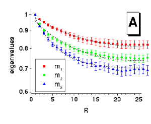
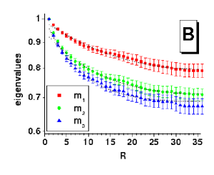
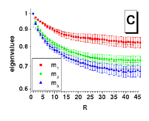
Figure 1: Eigenvalues of the cross-correlation matrix for $P^{\left(n\right)}$-operators with $n=\left\{3,9,15,21,27\right\}$. Panel A: $L_{S}=50$, panel B: $L_{S}=70$, panel C: $L_{S}=90,$

Mass	$L_{50}$	fit range	$L_{70}$	fit range	$L_{90}$	fit range
$M_{3}$	0.191(8)	[3,47]	0.134(3)	[2,68]	0.098(4)	[3,87]
$M_{2}$	0.107(3)	[2,48]	0.081(2)	[4,66]	0.058(2)	[5,85]
$M_{1}$	0.065(1)	[2,48]	0.0467(5)	[3,67]	0.0329(5)	[3,87]

Table 1: The screening-masses in lattice units (Mass) obtained by fitting the eigenvalues of the cross-correlation matrix of $P^{n}$-correlators by Eq.(18), with $n=\left\{3,9,15,21,27\right\}$ for lattices $L_{S}=\left\{50,70,90\right\}$. The ranges shown correspond to best-fits with goodness $\left(\chi\mathchoice{\hbox{{\texttwosuperior}}}{\hbox{{\texttwosuperior}}}{\hbox{{\texttwosuperior}}}{\hbox{{\texttwosuperior}}}/dof\right)_{L50}=0.306,$ $\left(R\mathchoice{\hbox{{\texttwosuperior}}}{\hbox{{\texttwosuperior}}}{\hbox{{\texttwosuperior}}}{\hbox{{\texttwosuperior}}}\right)_{L50}=0.993$; $\left(\chi\mathchoice{\hbox{{\texttwosuperior}}}{\hbox{{\texttwosuperior}}}{\hbox{{\texttwosuperior}}}{\hbox{{\texttwosuperior}}}/dof\right)_{L70}=0.139,$ $\left(R\mathchoice{\hbox{{\texttwosuperior}}}{\hbox{{\texttwosuperior}}}{\hbox{{\texttwosuperior}}}{\hbox{{\texttwosuperior}}}\right)_{L70}=0.997$ and $\left(\chi\mathchoice{\hbox{{\texttwosuperior}}}{\hbox{{\texttwosuperior}}}{\hbox{{\texttwosuperior}}}{\hbox{{\texttwosuperior}}}/dof\right)_{L90}=0.248,$ $\left(R\mathchoice{\hbox{{\texttwosuperior}}}{\hbox{{\texttwosuperior}}}{\hbox{{\texttwosuperior}}}{\hbox{{\texttwosuperior}}}\right)_{L70}=0.993$. Error-bars were computed by $70k$ bootstrap-repetitions performed over 1000 independent configurations. Integrated auto-correlation times $\left(\tau_{int-P}\right)$ associated to Polyakov loops $(i.e.\>P^{\left(0\right)})$ were used for checking the statistical independence of samples, they were computed by automatic windowing procedure with $c=[4,10]$. The error estimation for each $\tau_{int-P}$ is from Madras-Sokal formula [23], resulting in $\left(\tau_{int-P}\right)_{L50}=5366(645)$, $\left(\tau_{int-P}\right)_{L70}=9526(1013)$ and $\left(\tau_{int-P}\right)_{L90}=15108\left(1402\right)$.

We also performed a finite-size scaling (FSS) study using the measured masses ($m_{n}$) for extraction of their infinite-volume limit [42]. A fitting ansatz $m_{n}=a_{n}/L+b_{n}$ suggests $b_{n}\equiv 0$ for all masses, while $m_{n}=a_{n}L^{-\nu_{n}}$ corroborates with $v_{n}\equiv v$, within one standard-deviation. Thus, the following functional dependence

$$m_{n}=a_{n}L^{-\nu},$$ (19)

was employed for fitting simultaneously all data points, as is seen in Figure (2).

The obtained exponent $\nu=1.16(6)$ shows that at IR limit all mass-excitations $\left(m_{n}\right)$ scale as the inverse correlation-length $\left(\xi\right)$, as in the critical 2d Ising-model [26]. The average ratios computed from face values in Table (1), using error-propagation formulas, are compatible with results calculated from coefficients $a_{n}=[a_{1}=6.4(1.7),$ $a_{2}=10.7(2.9),$ $a_{3}=18.4(5.0)]$ from the best-fit (i.e. $\chi\mathchoice{\hbox{{\texttwosuperior}}}{\hbox{{\texttwosuperior}}}{\hbox{{\texttwosuperior}}}{\hbox{{\texttwosuperior}}}/dof=0.808,$ $R\mathchoice{\hbox{{\texttwosuperior}}}{\hbox{{\texttwosuperior}}}{\hbox{{\texttwosuperior}}}{\hbox{{\texttwosuperior}}}=0.993)$ with Eq.(19). Thus, it is pointed out that ratios for screening-masses in $0^{++}$ channel of the critical finite-temperature YM theory in $\left(2+1\right)d$ are $m_{2}/m_{1}=1.69(15)$ and $m_{3}/m_{1}=2.89(35)$.

Hence, the measured spectrum can be fitted by $b_{n}\equiv 0$, a behavior associated with a tower of massless excitations is seen at thermodynamic limit. Morever, our data agree with universality arguments Eq.(6) and, so far, the prediction Eq.(7) from mapping [15] stays valid for $d\neq 4.$

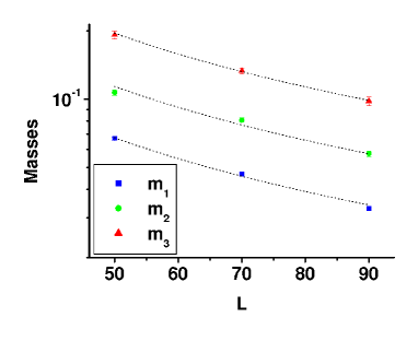
Figure 2: Scaling of effective-masses as a function of lattice sides $(L)$. Dot-line is the best global-fit from Ansatz in Eq.(19), its goodness is $(\chi\mathchoice{\hbox{{\texttwosuperior}}}{\hbox{{\texttwosuperior}}}{\hbox{{\texttwosuperior}}}{\hbox{{\texttwosuperior}}}/dof=0.808,$ $R\mathchoice{\hbox{{\texttwosuperior}}}{\hbox{{\texttwosuperior}}}{\hbox{{\texttwosuperior}}}{\hbox{{\texttwosuperior}}}=0.993)$. The exponent obtained $\nu=1.16(6)$ and the $\left(a_{n}\right)$ coefficients imply $0^{++}$ screening-mass ratios compatible with $m_{2}/m_{1}=1.69(15)$ and $m_{3}/m_{1}=2.89(35)$.

6 Concluding remarks

We have computed the gluonic spectrum of screening masses (in $0^{++}$ channel) of quenched $3d$ Yang-Mills theory at critical temperature. State-of-art techniques from hadron-spectroscopy, such as the variational-method and recursively-smeared interpolators, were employed with our new thermalization algorithm, to ensure accurate results at the critical region. While the measured spectrum is expected to present no significant systematic effects from UV-cutoff — since we employed very fine lattices — a noticeable dependence on the spatial lattice side (i.e. on the dimensionless quantity $L_{S}$) was observed.

Therefore, in the way to obtain the mass-excitations in the thermodynamic limit a FSS extrapolation was performed, which unveiled a tower of massless excitations, as expected by dynamical [15, 28] and universality-based arguments [5, 9, 10, 27] (i.e. similar to the spectrum of scalar/free-fermion field theories). A result that strongly resembles patterns from bound-states of glueballs analytically calculated for $SU(N)$ theories, at the $N\rightarrow\infty$ limit [43].

Hence, traditional criteria for confinement are based on the gauge-dependent behavior of gluon-propagators at the infrared limit [2]; connecting finite-temperature studies in different gauges [16] to gauge-independent [18] results is worthwhile. An analytical development in this direction was introduced in [15], where a mapping from $SU(N)$ gauge theories to $N-$scalar fields consistently fits $4d$ gluon-propagators at deep infrared. Moreover, it agrees with modern findings concerning YM theories for more general gauge groups [11], where a subtle dynamical balance among group generators and the size of group center seems to lead to occasional universal behavior.

Whether such assertions are valid for the finite-temperature $3d$ YM theory near criticality is a matter for numerical verification. So, we have computed mass-ratios of $SU(2)$ gauge theory and compared them to ratios from universality-related models, namely the $\lambda\phi^{4}$ and Ising-field theories. Our results match both universality and dynamical-mapping hypothesis [5, 9, 15, 28] in Eq.(6) and Eq.(7); which harmonizes with confinement-scenarios [29, 30, 44] presenting (confined) massive gluonic-excitations in $d>2$.

For future research we leave the computation of screening-masses for generalized YM theories [11] using smeared interpolators like Eq.(15), though built upon order parameters, as the dressed Polyakov-loop, associated with chiral Dirac operators [37, 46]. The resulting spectral patterns arising from such investigations could be straightforwardly related to the behavior of usual YM propagators by methods presented in [47], which may bring further insights into dynamical aspects connecting universality to chiral and deconfinement phase-transitions [48].

References

- [1] H. J. Rothe, Lattice Gauge Theories: an Introduction, World Scientific, (2005); T. Degrand and C. Detar, Lattice Methods For Quantum Chromodynamics, World Scientific, (2006).
- [2] R. Alkofer and L. Smekal, Phys. Rept. 353, 281 (2001).
- [3] F. Karsch, J. Phys.: Conf. Ser. 46, 122 (2006).
- [4] J. Z.-Justin, Quantum Field Theory and Critical Phenomena, Oxford University Press, (2002); M. Le Bellac, Quantum and Statistical Field Theory, Clarendon Press, (1994); M. Le Bellac, Thermal Field Theory, Cambridge University Press, (1996).
- [5] B. Svetitsky and L. Yaffe, Nucl. Phys. B 210, 423 (1982).
- [6] S. Fortunato, F. Karsch, P. Petreczky and H. Satz, Nucl. Phys. B (Proc. Suppl.) 94, 398 (2001).
- [7] J. Engels and T. Scheideler, Nucl. Phys. B 539, 557 (1999).
- [8] F. Gliozzi and P. Provero, Phys. Rev. D 56, 1131 (1997).
- [9] R. Fiore, A. Papa and P. Provero, Phys. Rev. D 67, 114508 (2003); R. Fiore, A. Papa and P. Provero, Nucl. Phys. B (Proc. Suppl.) 119, 490 (2003).
- [10] R. Falcone, R. Fiore, M. Gravina and A. Papa, Nucl. Phys. B 785 (2007) 19; R. Falcone, R. Fiore, M. Gravina and A. Papa, Nucl. Phys. B 767 (2007) 385.
- [11] K. Holland, M. Pepe and U.-J. Wiese, JHEP 0802, 041 (2008); M. Pepe and U.-J. Wiese, Nucl. Phys. B 768, 21 (2007); K. Holland, JHEP 0601, 023 (2006); K. Holland, M. Pepe and U. J. Wiese, Nucl. Phys. B 694, 35 (2004); K. Holland, M. Pepe and U.-J. Wiese, Nucl. Phys. Proc. Suppl. 129, 712 (2004).
- [12] A. C. Aguilar and A. A. Natale, JHEP 0408, 057 (2004).
- [13] R. Alkofer, M. Q. Huber and K. Schwenzer, [arXiv:0801.2762].
- [14] A. Cucchieri and T. Mendes, Phys. Rev. D 78, 094503 (2008); A. Cucchieri and T. Mendes, Phys. Rev. Lett. 100, 241601 (2008); A. Cucchieri and T. Mendes, PoSLAT2007, 297 (2007).
- [15] M. Frasca, Phys. Lett. B 670, 73 (2008); M. Frasca, Int. J. Mod. Phys. A 22, 1727 (2007); M. Frasca, [arXiv:0903.2357].
- [16] A. Cucchieri, A. Maas and T. Mendes, Phys. Rev. D 75, 076003 (2007); A. Cucchieri, F. Karsch and P. Petreczky, Phys. Lett. B 497, 80 (2001); A. Cucchieri, F. Karsch and P. Petreczky, Nucl. Phys. Proc. Suppl. 94, 385 (2001); A. Cucchieri, F. Karsch and P. Petreczky, Phys. Rev. D 64, 036001 (2001).
- [17] J. Erlich, PoS Confinement8, 032 (2008). And references therein.
- [18] Y. Maezawa, S. Aoki, S. Ejiri, T. Hatsuda, N. Ishii, K. Kanaya, N. Ukita and T. Umeda, PoSLAT2008, 194 (2008).
- [19] A. Cucchieri, Nucl. Phys. B 508, 353 (1997).
- [20] X.- F. Meng, G. Li, Y. Chen, C. Liu, Y.-B. Liu, J.-P. Ma and J.-B. Zhang, [arXiv:0911.4869]; N. Ishii and H. Suganuma, [arXiv:hep-lat/0312040]; N. Ishii., H. Suganuma and H. Matsufuru, [arXiv:hep-lat/0212010]; N. Ishii, H. Suganuma and H. Matsufuru, Phys. Rev. D 66, 094506 (2002); N. Ishii, H. Suganuma and H. Matsufuru, Phys. Rev. D 66, 014507 (2002); B. Grossman, S. Gupta, U. M. Heller and F. Karsch, Nucl.Phys. B 417, 289 (1994); M. Loan and Y.- Ying, Prog. Theor. Phys. 116, 169 (2006); H. B. Meyerand and M. J. Teper, Nucl. Phys. B 668, 111 (2003); J. Carlsson and B. H. J. McKellar, [arXiv:hep-lat/0303018]; J. Carlsson and B. H. J. McKellar, Phys. Rev. D 68, 074502 (2003); H. B. Meyer and M. J. Teper, Nucl. Phys. B 658, 113 (2003); Da Q.- Liu, J.- M. Wu and Y. Chen, Nucl. Phys. 26, 222 (2002). And references therein.
- [21] C. Michael, Nucl. Phys. B 259, 58 (1985); M. Lüscher and U. Wolff, Nucl. Phys. B 339, 222 (1990); A. S. Kronfeld, Nucl. Phys. (Proc. Suppl.) 17 (1990) 313.
- [22] R. B. Frigori, A. Cucchieri, T. Mendes and A. Mihara, AIP Conf. Proc. 739, 593 (2005); A. Cucchieri, R. B. Frigori, T. Mendes and A. Mihara, Braz. J. Phys. 36, 631 (2006).
- [23] A. D. Sokal, Monte Carlo methods in statistical mechanics: foundations and new algorithms, Lectures at Cargèse summer school, (1996); U. Wolff, Comput. Phys. Commun. 156, 143 (2004); Erratum-ibid. 176, 383 (2007).
- [24] A. Cucchieri and T. Mendes, [arXiv:0904.4033v1]; A. Sternbeck and L. von Smekal, PoSLAT2008, 267 (2008).
- [25] A. M. Polyakov, Phys. Lett. B 72, 477 (1978).
- [26] A. Pelissetto and E. Vicari, Phys. Rep. 368, 549 (2002).
- [27] G. Delfino, J. Phys. A 37, R45 (2004); T. T. Wu, B. M. McCoy, C. A. Tracy and E. Barouch, Phys. Rev. B 13, 316 (1976).
- [28] M. Frasca, Int. J. Mod. Phys. A 22, 1441 (2007); M. Frasca, Phys. Rev. D 73, 027701 (2006) and Erratum-ibid. D 73, 049902 (2006); M. Frasca, Int. J. Mod. Phys. A 22, 2433 (2007); M. Frasca, Int. J. Mod. Phys. A 22, 5345 (2007).
- [29] S. P. Sorella, Phys. Rev. D 80, 025013 (2009); D. Dudal, S. P. Sorella, N. Vandersickeland and H. Verschelde, [0808.3379].
- [30] A. Maas, Phys. Rev. D 75, 116004 (2007).
- [31] M. Creutz, Phys. Rev. D 21, 2308 (1980).
- [32] A. D. Kennedy and B. J. Pendleton, Phys. Lett. B 156, 393 (1985).
- [33] R. Petronzio and E. Vicari, Phys. Lett. B 254, 444 (1991).
- [34] S. L. Adler, Nucl. Phys. Proc. Suppl. 9, 437 (1989).
- [35] G. P. Lepage, B. Clark, C. T. H. Davies, K. Hornbostel, P. B. Mackenzie, C. Morningstar and H. Trottier, Nucl. Phys. Proc. Suppl. 106, 12 (2002); C. Morningstar, Nucl. Phys. Proc. Suppl. 109 A, 185 (2002).
- [36] G. M. Hippel, R. Lewis and R. G. Petry, Comput. Phys. Commun. 178, 713 (2008).
- [37] C. Gattringer, C. Hagen, C. B. Lang, M. Limmer, D. Mohler and A. Schäfer, Phys. Rev. D 79, 054501 (2009); R. B. Frigori, Ch. Gattringer, C. B. Lang, M. Limmer, T. Maurer, D. Mohler, and A. Schäfer, PoSLAT2007, 114 (2007); T. Burch, C. Gattringer, L. Ya. Glozman, C. Hagen, D. Hierl, C. B. Lang and A. Schäfer, Phys. Rev. D 74, 014504 (2006).
- [38] J. M. Bulava, R. G. Edwards, E. Engelson, B. Joó, A. Lichtl, H-W. Lin, N. Mathur, C. Morningstar, D. G. Richards and S. J. Wallace, Phys. Rev. D 79, 034505 (2009).
- [39] C. Legeland, J. Engels, F. Karsch, E. Laermann, M. Lütgemeier, B. Petersson and T. Scheideler, Nucl. Phys. B (Proc. Suppl.) 53, 420 (1997).
- [40] M. Teper, Phys. Rev. D 59, 014512 (1999).
- [41] A. Cucchieri, T. Mendes and A. Taurines, Phys. Rev. D 67, 091502 (2003).
- [42] N. A. Alves, B. A. Berga and R. Villanova, Phys. Rev. B 43, 5846 (1991).
- [43] B. H. J. McKellar and J. Carlsson, Nucl. Phys. B (Proc. Suppl.) 129&130, 420 (2004).
- [44] M. Chaichian and K. Nishijima, Eur. Phys. J. C 47, 737 (2006).
- [45] S. Edwards and L. von Smekal, Phys. Lett. B 681, 484 (2009).
- [46] F. Bruckmann, E. Bilgici, C. Gattringer and C. Hagen, PoS Confinement8, 054 (2008).
- [47] J. Danzer, C. Gattringer and A. Maas, JHEP 0901, 024 (2009); A. Maas and S. Olejnik, JHEP 0802, 070 (2008).
- [48] T. Mendes, PoSLAT2007, 208 (2007).