On type I cascaded quadratic soliton compression in lithium niobate: Compressing femtosecond pulses from high-power fiber lasers
Abstract
The output pulses of a commercial high-power femtosecond fiber laser or amplifier are typically around 300-500 fs with a wavelength around 1030 nm and 10s of J pulse energy. Here we present a numerical study of cascaded quadratic soliton compression of such pulses in LiNbO3 using a type I phase matching configuration. We find that because of competing cubic material nonlinearities compression can only occur in the nonstationary regime, where group-velocity mismatch induced Raman-like nonlocal effects prevent compression to below 100 fs. However, the strong group velocity dispersion implies that the pulses can achieve moderate compression to sub-130 fs duration in available crystal lengths. Most of the pulse energy is conserved because the compression is moderate. The effects of diffraction and spatial walk-off is addressed, and in particular the latter could become an issue when compressing in such long crystals (around 10 cm long). We finally show that the second harmonic contains a short pulse locked to the pump and a long multi-ps red-shifted detrimental component. The latter is caused by the nonlocal effects in the nonstationary regime, but because it is strongly red-shifted to a position that can be predicted, we show that it can be removed using a bandpass filter, leaving a sub-100 fs visible component at nm with excellent pulse quality.
pacs:
42.65.Re, 42.65.Ky, 05.45.Yv, 42.70.Mp, 42.65.Hw, 42.65.Jx, 42.65.JxI Introduction
Pulsed fiber laser systems are currently undergoing a rapid development, and by employing the chirped pulse amplification (CPA) technique high-energy femtosecond pulses can be generated with J–sub-mJ pulse energies fermann:2009 . Combined with the fact that the fiber laser technology offers a rugged, cheap and compact platform, ultrafast fiber CPA (fCPA) systems could compete with solid-state amplifier systems. However, the gain bandwidth of the Yb-doped fibers typically used for lasing in the region is considerably lower than competing solid-state materials (such as Ti:Sapphire crystals). Thus, due to the build up of an excessive nonlinear phase shift Yb-based fCPA lasers are often limited to a pulse duration that typically is sub-ps at best (around fs) for J pulses limpert:2006 while shorter pulses can be reached ( fs) for J pulses Kuznetsova:2007 .
Efficient external compression methods are therefore needed. A prototypical compressor consists of a piece of nonlinear material, where a broadening of the pulse bandwidth occurs by self-phase modulation (SPM), followed by a dispersive element (gratings or chirped mirrors) that provides temporal compression. With this method (using a short piece of fiber as nonlinear material) 27 fs sub-J pulses were generated from 270 fs 0.8 J pulses from an fCPA system eidam:2008 . Alternative methods consist of using long (0.5 m or more) gas cells or filaments nisoli:1996 ; *hauri:2004 as nonlinear material, and this works with pulse energies from 50 J to around 1 mJ (limited in part by self-focusing effects) or possibly even higher energies Chen:2008 .
Using soliton compression both the SPM-induced pulse broadening and dispersion-induced compression occur in the same material mollenauer:1980 . However, as self-focusing solitons require anomalous dispersion this can only be achieved in the near-IR through strong waveguide dispersion. This means using specially designed fibers, such as micro-structured fibers. Fibers have a very limited maximum pulse energy of a few nJ, albeit large mode-area micro-structured solid-core and hollow-core fiber compressors can support up to 1 J Ouzounov:2005 ; *Laegsgaard:2009.
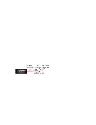
Unfortunately the pulse energy from fCPA systems lies exactly in the gap between these methods. We will here study a compression method that can compensate for this. It is a soliton compressor based on cascaded quadratic nonlinearities liu:1999 ; ashihara:2002 ; wise:2009 , see Fig. 1. This has several advantages: As it relies on a self-defocusing nonlinearity, there are no problems with self-focusing effects, and multi-mJ pulse-energies can be compressed. Moreover, solitons require normal instead of anomalous dispersion, implying that solitons can be generated in the visible and near-IR. Finally, it is extremely simple as it relies on just a small piece of quadratic nonlinear crystal, preceded only by a lens or a beam expander moses:2007 .
The basis for the cascaded quadratic soliton compressor (CQSC) is phase-mismatched second-harmonic generation (SHG). The cascaded energy transfer from the pump (fundamental wave, FW) to the second harmonic (SH) and back imposes a strong SPM-like nonlinear phase shift on the FW, whose sign can be made self-defocusing desalvo:1992 ; stegeman:1996 . Thereby the FW pulse can be compressed with normal dispersion liu:1999 , and soliton compression becomes possible in the visible and near-IR ashihara:2002 .
In this paper we investigate the CQSC in a type I lithium niobate (LiNbO3, LN) crystal, where the goal is to perform moderate compression of longer fs pulses from fCPA systems at the Yb gain wavelength of 1030 nm. We show that in order to overcome the detrimental cubic nonlinearities the phase mismatch has to be chosen so low so that the compression occurs in the so-called nonstationary regime. This regime is dominated by group-velocity mismatch (GVM) effects, and exactly the large GVM is a well-known drawback of using LN in the near-IR for SHG. However, when only moderate compression is desired, the soliton order can be kept low, and we show through numerical simulations that reasonable pulse quality can be achieved and that up to 80% of the pulse energy is retained in the central spike. The compression limit is found to be around 120 fs FWHM, which is a limit set by the GVM effects. The compression occurs in a crystal of reasonable length, 10 cm. This is possible only because LN has a very large 2. order dispersion. Finally, we show that bandpass filtering of the SH actually can lead to a very clean sub-100 fs visible pulse with around 0.1% conversion efficiency.
In this paper we first discuss the general compression properties of LN in a cascaded type I SHG interaction setup in Sec. II, and then show some numerical simulations in Sec. III of pulses coming from two different commercially available fCPA systems. We conclude in Sec. IV. The properties of LN are discussed in App. A, and App. B discusses the anisotropic Kerr nonlinear response of LN. Appendix C and D discuss the conversion relations between Gaussian and SI units for cubic nonlinear coefficients and Miller’s rule, respectively.
II Type I compression properties of lithium niobate crystals
With the CQSC high-energy few-cycle compressed pulses can be generated, as was experimentally observed at 1250 nm moses:2006 . However, the first studies performed at 800 nm were plagued by GVM effects, that prevented reaching the few-cycle regime liu:1999 ; moses:2006 ; ashihara:2002 . These studies used a -barium–borate (BBO) crystal in a type I SHG configuration, where the FW (ordinary polarization) is orthogonal to the SH (extraordinary polarization) and where birefringent phase matching is possible by angle-tuning the crystal. BBO is in many respects an ideal nonlinear crystal: it has low dispersion, a very large transparency window, and a reasonably strong quadratic nonlinearity relative to the detrimental cubic one. As we have shown in previous theoretical and numerical studies, BBO provides an excellent compression of longer pulses to ultra-short duration at the Yb gain wavelengths bache:2007a ; bache:2007 ; bache:2008 . The problem with BBO is that good quality waveguides are not supported and that it is very difficult to grow long crystals. Especially the latter is important if only moderate compression of longer pulses is desired. In moderate soliton compression most of the pulse energy is conserved in the compressed pulse, and the pulse has a reduced pedestal. The problem is that compression will only occur after a long propagation length.
We therefore turn here to LN, which is a widely used quadratic nonlinear crystal for IR frequency conversion. LN is attractive due to extremely large effective quadratic nonlinearities (up to 10 times larger than BBO), that can be accessed through a quasi-phase matched (QPM) type 0 SHG phase matching configuration where FW and SH have identical polarization. However, here we study LN in a type I configuration as BBO. The effective quadratic nonlinearity is more than twice as large as in BBO.
LN is usually not considered very suitable for SHG of short pulses in the near-IR because the SH becomes very dispersive; thus, the FW and SH group velocities are very different resulting in large GVM. This is also why LN has not been used in the near-IR as nonlinear medium for the CQSC, for which GVM is a very detrimental effect. Another disadvantage for the CQSC is that the Kerr nonlinear response is several times larger than BBO, which counteracts the advantage of the large quadratic nonlinearity of LN. Therefore the CQSC experiments done so far using LN were done in the telecommunication band and exploited QPM in a type 0 configuration ashihara:2004 ; *zeng:2006, where effective quadratic nonlinearity is around three times larger than what can be achieved in a type I configuration. However, we now show that type I LN offers a quite decent compression performance without having to custom design a QPM grating.
II.1 Solitons with cascaded quadratic nonlinearities
In cascaded quadratic interaction the FW effectively experiences a Kerr-like nonlinear refractive index. This is in addition to the cubic (Kerr) nonlinearities that are always present in all media. We can write the total refractive index of the FW [see Eq. (32)]
| (1) |
where is the FW linear refractive index, is the FW electric field, and the FW intensity. It is typical to report the nonlinear refractive index relative to the electric field, , or to the intensity, . We have here for simplicity neglected cross-phase modulation (XPM) contributions since they are small in cascaded SHG. As mentioned we have contributions from both cascaded quadratic and cubic Kerr nonlinearities
| (2) |
where is the SPM Kerr nonlinear refractive index of the FW (see App. B for details on the notation etc.). The contribution from the cascaded quadratic nonlinearities can in the large phase mismatch limit (, where is the crystal length) be approximated as desalvo:1992
| (3) |
where is the effective nonlinearity. For the cascaded contribution is negative, i.e. self-defocusing. Here is the wavenumber.
The effective quadratic nonlinearity of the type I interaction for the crystal class (LN, BBO) is
| (4) |
where the angles are defined in Fig. 9 in App. B. Choosing gives maximum nonlinearity (see App. A).
In cascaded quadratic soliton compression the aim is to get and as to achieve a total self-defocusing cubic nonlinearity. The soliton interaction can then be described by an effective soliton order bache:2007
where is the soliton order of the self-defocusing cascaded quadratic nonlinearity, and is the soliton order of the material Kerr self-focusing cubic nonlinearity. The FW dispersion length is , where is the FW group-velocity dispersion (GVD). We generally use the following notation for the dispersion parameters .
II.2 Linear and nonlinear response of LN at
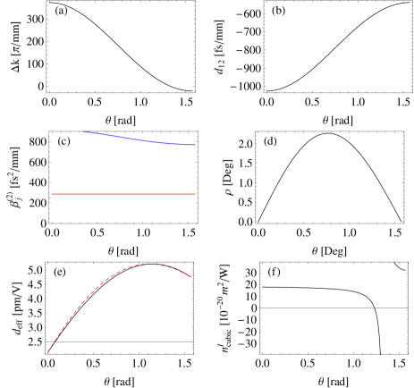
Selecting , the operating wavelength of most Yb-based fiber laser amplifiers, the properties of LN are summarized in Fig. 2: the phase mismatch (a) becomes small at radians (). As shown in (e) in this range pm/V, and the total nonlinear refractive index (f), as expressed by Eq. (2), can become negative, implying that the cascaded nonlinearity is stronger than the Kerr nonlinearity. This happens for (or ). At phase matching is achieved, after which and thus self-focusing.
GVM is very large, see Fig. 2(b), which as we will see later sets a strong limitation to the compression performance. The GVD is shown in Fig. 2(c), and importantly FW GVD (red) is large and normal (i.e. positive). It will stay normal until m, after which it becomes anomalous and self-defocusing solitons are no longer supported. The SH GVD (blue) is about 3 times larger than the FW GVD.
Since the type I critical phase matching is employed, the walk-off angle (valid for a negative uniaxial crystal) is nonzero, see Fig. 2(d). In Fig. 2(e) it is apparent that is largely unaffected by walk-off. However, walk-off does set a limit to the effective interaction length between the pump and the SH as we will discuss later.
II.3 Compression diagram for type I LN
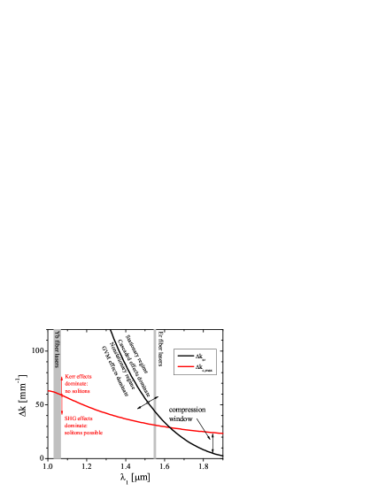
We now generalize to other wavelengths and summarize the type I compression performance of LN in Fig. 3 111The specific crystal chosen in this work is 1% MgO doped stoichiometric LN, as the MgO doping gives a much higher material damage threshold. Also 5% MgO doped congruent LN would work well. See App. A for more details about the crystal.. This compression diagram shows the different compression regimes for the CQSC as the wavelength and the phase mismatch is varied.
Above the red curve the total nonlinear refractive index is focusing , so solitons are not supported since the FW GVD is normal. The curve is found by setting giving bache:2007
| (6) |
Below the black curve the compression performance is dominated by GVM effects (nonstationary regime) while above it is dominated by cascaded effects (stationary regime). The curve is to second order 222A more accurate transition can easily be calculated numerically using the full SH dispersion operator bache:2008 , which we have done in what follows. given by bache:2007a
| (7) |
where is the GVM parameter and is the SH GVD. The lower this curve is the better because this implies that the chance of observing solitons in the stationary regime increases. Thus, the very large GVM parameter is detrimental because it pushes the curve upwards. Instead the huge SH GVD values, see Fig. 2 (c), are actually helping to push the curve downwards. Therefore a large SH GVD can actually be beneficial for clean soliton compression.
The optimal compression occurs in the so-called “compression window” bache:2007a , where the soliton compressor works most efficiently because solitons are supported in the stationary regime. The diagram shows a compression window for type I LN in the regime m. Unfortunately in this range there are no fCPA systems.
Fortunately, as we will show also in the nonstationary regime compression is possible, as long as the effective soliton order is low enough. This is what we will try to exploit in the regime around m.
Coming back to we observe that solitons are supported for when . However, when getting too close to the intensities required to observe solitons become very large implying excessive Kerr XPM effects and increased Raman-like GVM effects bache:2008 . On the other hand for too small the cascading limit ceases to hold, and also the compressor performance decreases due to excessive GVM effects bache:2008 . In fact, as a rule of thumb the compression limit in the nonstationary regime (in which the system will always be for ) the compression limit is roughly given by the pulse duration for which , where is the coherence length and is the dynamic GVM length of a sech-shaped soliton. With “dynamic” we mean that the GVM length changes as the soliton compresses. Thus, in the nonstationary regime the limit is 333Note that this expression differs with a factor of from the limit that we suggested in bache:2008 ; this is purely an empirical choice.
| (8) |
where the factor in front of the fraction is the conversion factor to FWHM for a sech-shaped pulse. Obviously as approaches the phase matching point the soliton cannot compress to short durations. We numerically found the optimal compression point in the regime, and with the best results for , for which .
II.4 Predicting the compression performance
The next step is to estimate what the compression performance could look like. Here the scaling laws 444Note that the scaling laws presented here are only ball-park figures when used in the nonstationary regime as they were found in the stationary regime. come into the picture, which can be used to predict the propagation distance for optimal compression , the compression factor and the pulse quality bache:2007 .
As we have pointed recently bache:2007a , it is the phase mismatch and the GVM (zero and first order dispersion) that really control the compression properties. The only requirement to the second order dispersion is that FW GVD is normal as to support solitons. Otherwise as we discuss below the FW GVD is basically just determining the optimum compression length. The SH GVD instead plays a minor role in the compression properties, cf. Eq. (7). Our initial idea was to exploit that LN is quite dispersive when pumped at m, so the very large FW GVD makes it possible to compress the pulse in a short crystal.
So why and when is it interesting to increase GVD as to compress in a short crystal? Obviously, the crystals have length limits, which for LN is around 100 mm. The optimal compression point scales as bache:2007
| (9) |
where is the soliton length agrawal:1989 . So the point where the pulse compression is optimal depends on the effective soliton order, the input pulse duration and the FW GVD. Therefore since quality LN crystals are maximum 100 mm long, the CQSC works best when the soliton order is large and the GVD length is short. But when the soliton order is large, the detrimental effects due to GVM are strongly increased moses:2006 ; bache:2008 , in particular in the nonstationary regime. Therefore, in the case we study here clean compression can only be done with low soliton order, and therefore the FW GVD must be large as to ensure compression in realistic crystal lengths.
A downside to the large GVD is the following: given that some effective soliton order is required then since we have that a large GVD gives a short GVD length, and thus larger intensities are needed to excite a soliton. The same problem is found for short input pulses, say from a Ti:Sapphire amplifier. However, this is only an issue if operating with intensities close to the damage threshold, which is not the case here: the intensities are moderate (), and instead our issue is to get the solitons to compress in a crystal that is not too long.
The compression factor , where is the pulse compressed pulse duration at , is also affected by the effective soliton order bache:2007
| (10) |
The pulse quality can also be predicted, and is defined as the ratio between the compressed pulse fluence with that of the input pulse. It scales as bache:2007
| (11) |
We can use this to calculate the compressed pulse peak intensity and energy . An advantage of using low soliton orders is that remains high, and thus the compressed pulse retains most of the initial pulse energy.
II.5 Compression performance of fCPA systems
Let us use these scaling laws to predict the compression performance of fCPA systems. High-energy femtosecond pulses from fCPA systems use both Yb doped and Er doped gain fibers. Since fCPA systems are diode pumped with a wavelength just below the quantum efficiency of Yb doped systems is higher, and therefore the majority of commercial and scientific systems prefer to use Yb over Er. Most systems operate at the Yb emission line and can for low pulse energies (J) generate pulses as short as 250 fs, while higher pulse energies result in longer pulses (currently J 450 fs pulses is the state-of-the-art for commercial systems). In Er amplifier systems much lower pulse energies are available, typically J and fs pulses at ; such low pulse energies and long pulse duration mean that only very low soliton orders can be excited, and thus the CQSC can only achieve very moderate compression occurring in very long crystals.
The basis for the following case studies and numerical simulations is therefore a couple of commercially available Yb-based fCPA systems, both operating at 1030 nm. Case (1) is a Clark MXR Impulse 555\htmladdnormallinkhttp://www.clark-mxr.com http://www.clark-mxr.com giving 15 J 250 fs FWHM pulses, which represents a system giving quite short, yet still reasonably energetic pulses as a starting point. Case (2) is an Amplitude Systemes Tangerine 666\htmladdnormallinkhttp://www.amplitude-systemes.com http://www.amplitude-systemes.com giving 50 J 450 fs FWHM pulses, which represents a system with more energetic but also longer pulses.
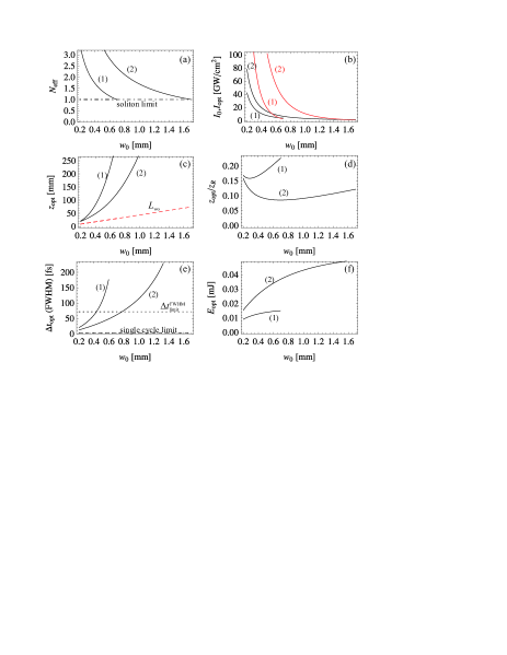
The two cases are studied together taking . Figure 4(a) shows that in case (1) we need to focus the pulses to to observe solitons: in this regime Fig. 4(d) shows that the Rayleigh length is only 5-6 times larger than the optimal compression point of around 100 mm. This is borderline at the risk of experiencing diffraction problems. Even increasing or decreasing the waist does not improve this ratio much. In case (2) instead, the increased pulse energy makes solitons appear already at mm, despite the longer pulse duration. This means that diffraction should be less of an issue: in Fig. 4(d) the pulse compression point relative to the Rayleigh length of the focused beam is significantly smaller in case (2).
Fig. 4(c) indicates that the spatial walk-off in the crystal can become an issue: the crystal should be shorter than the spatial walk-off length to ensure proper interaction between the FW and the SH, but evidently the pulse compression lengths in both cases are at least a factor of 2-3 longer than the spatial walk-off length. It might therefore be necessary to compensate for this by using two crystals, one inverted relative to the other so the walk-off direction in the 2. crystal is inverted with respect to the 1. crystal Zondy:1994 .
An alternative solution to the walk-off problem is to turn to a noncritical phase matching scheme, where . This happens for or , see Fig. 2(d). Of course this removes the possibility of tuning the phase matching via , and one has to turn to temperature tuning of . The temperature needed to get to the desired operation point () can be estimated using the temperature dependent Sellmeier equations gayer:2008 , and our calculations indicate that it should happen already at a temperature of around C. This would make an easy solution to the walk-off problem.
The strong GVM implies that compression of Yb-based systems can only occur in the nonstationary regime, see Fig. 3. Thus, unless is close to unity the GVM induced Raman-like effects dominate, and the FW pulse becomes extremely distorted and very poorly compressed. Actually, as a rule of thumb it never makes sense to use larger than what is sufficient to reach the limit expressed by Eq. (8), and typically even an smaller than that. The limit is drawn as a dotted line in Fig. 4(e), and it is reached around in case (1) and in case 2.
III Numerical simulations
We here present numerical simulations of the two cases using a plane-wave temporal model based on the slowly evolving wave equation (see more details in bache:2007 and references therein), which includes self-steepening effects and higher-order dispersion. This model is justified as long as diffraction is minimal, which we assume is the case when the crystal length is much shorter than the Rayleigh length, and when spatial walk-off is minimal. This requirement will be discussed further below.
III.1 Case (1): 250 fs 15 J pulses
For the 250 fs J pulses from a Clark laser system we found that the best compression was obtained with . This soliton order can be achieved with 15 J pulse energy when the pump is focused to around , see Fig. 4(a).
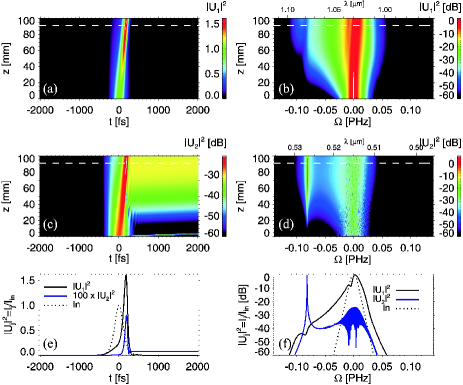
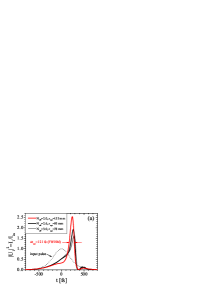
The theoretical compression factor for such soliton orders is , i.e., a fs FWHM compressed pulse is predicted. In Fig. 5 we show the results of a simulation with . This soliton order gave the best compression: a slightly asymmetric fs (FWHM) pulse is observed after 91 mm of propagation, see (a) and cut in (e). The compression is not quite as strong as predicted by the scaling law (10), but this is because the scaling laws are based on pulse compression in the stationary regime. On the other hand the pulse quality is large, , so most of the pulse energy is retained in the central compressed part, and the pulse pedestal is also very small. These are the main advantages of soliton compression with low soliton orders.
The FW spectrum (b) experiences upon propagation SPM-like broadening, where the blue-shifted shoulder clearly dominates; this is a sign of the cascaded quadratic nonlinearities dominating, and the fact that it is blue shifted is related to the negative sign of .
In the SH time-plot (c) we observe the strong GVM first inducing a weak component quickly escaping from the central part of the pulse, and later the GVM induces the characteristic DC-like trailing temporal pulse in the SH (this often occurs close to or at phase matching in presence of GVM, see also Noordam:1990 ; bakker:1992 ; Su:2006 ). This behaviour is also reflected in the SH spectrum, see (d) and cut in (f), which shows a very strong and extremely narrow red-shifted component building up, which eventually becomes the dominating contribution. As we discuss below its spectral position can accurately be predicted by the nonlocal theory that was recently developed by us bache:2007a ; bache:2008 . We believe that this strong and long SH trailing component actually causes the trailing part of the FW to be strongly depleted, and that this is the main reason for the asymmetrical FW shape.
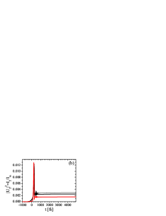
The question is now: can we increase the effective soliton order and achieve further compression below 100 fs as to approach the limit predicted by Eq. (8)? This turns out to be impossible: when is increased the GVM effects become stronger, making the compressed pulse more distorted. This is clearly observed in Fig. 6, where we increase and compare with the compression of Fig. 5: For the compressed FW pulse in (a) is still quite short, but clearly is less clean. For the compressed pulse instead becomes quite distorted. It is also evident in the SH time plots that the trailing DC-like component increases with , while the central part in all cases is a sub-100 fs FWHM pulse. It is quite weak because most of the converted SH energy is fed into the DC-like part of the pulse, which is connected to the strong spectral peak in the SH spectrum. This spectral peak becomes stronger with increased (not shown), but does not change position as it does not dependent on .
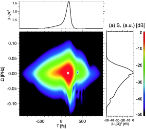
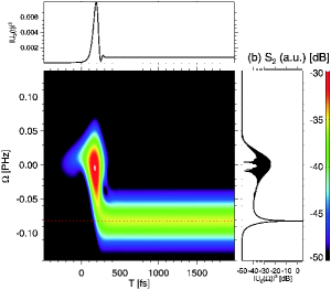
In order to understand the spectral content of the different temporal components, the cross-correlation frequency-resolved optical gating (XFROG) method is useful. The spectral strength is given by linden:1998
| (12) |
where is a properly chosen gating pulse. The spectrograms of the compressed pulses in Fig. 6 for are shown in Fig. 7. The FW compressed pulse is slightly blue-shifted (around 2 THz), and the compressed part (located at fs) shows a significantly broader spectrum.
The SH spectrum is very particular: the part of the pulse that propagates with the FW group velocity (the “locked” part) shows a quite clean short pulse. This group velocity locking of the SH has been observed before Noordam:1990 ; *bakker:1992; *Su:2006; ashihara:2004 and can be understood from the nonlocal theory bache:2007a ; bache:2008 : the SH has a component that is basically slaved to the FW due to the cascading nonlinearities. In frequency domain it can be compactly expressed as bache:2008
| (13) |
where denotes the forward Fourier transform, and are properly normalized fields. Thus, the spectral content of the SH is slaved to the spectral content of the spectrum of . The weight is provided by the nonlocal Raman-like response function in the nonstationary regime bache:2008
| (14) |
where . These frequencies can be calculated (to 2. order) from the dispersion of the system as PHz and PHz. In the center around , where is residing in this case, the response is quite flat: thus we get a SH component locked to the FW and when the FW compresses so does this SH component.
Another striking feature of the SH spectrogram is the DC-like component: it is very evident as a long pulse centered around THz. Also this peak can be understood from Eq. (13), because according to Eq. (14) the nonlocal response function in the nonstationary regime has sharp resonance peaks in the response at . Inserting the dispersion values of the simulation we get THz in excellent correspondence with the observed peak position as the red dashed line indicates. Instead is located too far into the red side of the spectrum to affect the behaviour.
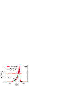
Considering this spectral composition, it might even be possible to filter away the disturbing SH component at , which in time-domain would give a quite decent SH pulse. In (c) we show that this is feasible: we pass the SH pulse through a super-Gaussian () bandpass filter centered at and with a bandwidth of 100 THz FWHM (corresponding to 15 nm): this filters away the disturbing sharp peak, and a 80 fs FWHM pulse remains at nm. The peak intensity in this short pulse is around . If we assume that it is created with 15 J pulse energy focused to mm to achieve , and that the generated SH has roughly the same spot size, then the pulse energy of the filtered 80 fs pulse would be around 50 nJ.
III.2 Case (2): 450 fs 50 J pulses
In case (2) the pulse duration is longer, 450 fs. When the pulse duration is longer the soliton will for a fixed soliton order compress after a longer distance. This is because according to Eq. (9) . However, we may compensate for this by increasing the effective soliton order enough to reach the limit governed by Eq. (8). For a 450 fs 50 J pulse it is achieved around mm, see Fig. 4(e), resulting in . This higher soliton order should make it possible to compress in crystal lengths of around 10-15 cm, see Fig. 4(c).
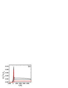
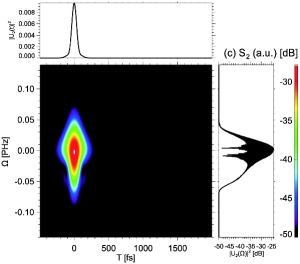
In Fig. 8 we show some numerical simulations using these longer more energetic pulses. The best pulse observed shows a three-fold compression to fs (FWHM) at . The compression occurred after around 15 cm propagation, so spatial walk-off would be an issue here. Increasing the soliton order to the pulse becomes more distorted, but still compresses to around 150 fs FWHM after 9.5 cm, a more realistic interaction length. Finally, at the pulse becomes too distorted as the GVM effects become stronger.
In the two cases the pulses therefore eventually compress to the same duration, which is the limit imposed by the nonlocal GVM effects. The more energetic pulses in case (2) allow for a more defocused pump beam so the compression should be less affected by diffraction. On the other hand, as the pulses are longer they compress later, so spatial walk-off is a more severe issue. A more optimal situation in both cases would therefore be more energetic pulses so the pump can be defocused with a factor 2-3. This would diminish spatial walk-off effects.
IV Conclusion
Here we have shown that lithium niobate (LN) crystals in a type I cascaded SHG interaction can provide moderate compression of fs pulses from Yb-based fiber amplifier systems ( wavelength). The phase mismatch was controlled through angle tuning (critical phase matching interaction). Using numerical simulations we found that the best compression was to around 120 fs FWHM after around 10 cm propagation.
Better compression was prevented in part by strong GVM effects, caused by strong dispersion in the LN crystal, and competing material Kerr nonlinear effects. These are focusing of nature and counteract the defocusing Kerr-like nonlinearities from the cascaded SHG. In order to make the total nonlinear phase shift negative the phase mismatch had to be taken quite low, and in this regime GVM effects dominate (the “nonstationary” regime). GVM imposes a strongly nonlocal temporal response in the cascaded nonlinearity that feeds most of the converted energy into a narrow red-shifted peak. In the temporal trace this gave a SH with a multi-ps long trailing component. The FW therefore experienced a distorted compression less the soliton order was kept very low. For such low soliton orders the compression distance increases substantially, but here the strong dispersion of the LN crystal actually becomes an advantage: due to a large GVD the soliton dynamics occur in much shorter crystals than usual, and the numerics indicated compression in realistic crystal lengths (10 cm).
It was noted that using low soliton orders gave a compressed pulse retaining most of the input pulse energy (in the cases we showed around 80%), and that the unavoidable soliton pedistal was less pronounced.
We also discussed the implications of using long crystals. Spatial walk-off will be an issue since it is a critical phase matching scheme is used that exploits birefringence, and also diffraction can be a problem. In order to counteract these detrimental effects the pump pulses need to be as energetic and short as possible. Two cases were highlighted taken from commercially available systems, and we argued that diffraction should not prevent observing the predicted compression, but that some sort of walk-off compensation might be needed. Future systems with more energetic pulses and reasonably short pulse durations ( fs) would be able to beat the walk-off problem. Walk-off could also be prevented by using a noncritical type I phase matching scheme () and increasing the temperature slightly to around C.
We finally noted that the peculiar SH shape in the nonstationary regime gave a very characteristic spectrogram: as mentioned above nonlocal GVM effects resulted in a sharp spectral red-shifted peak with a long multi-ps trailing temporal component. Another pulse component was instead locked to the group velocity of the compressed FW soliton. This locked visible pulse was located at the SH wavelength (515 nm), quite far from the red-shifted peak. We showed that a simple bandpass filter could actually remove the detrimental red-shifted peak leaving a very clean 80 fs visible pulse ( nm). This is the opposite approach compared to other studies, see e.g. bakker:1992 ; Marangoni:2007 , where focus was on exploiting “spectral compression” of fs pulses to obtain longer ps pulses. Despite that the cascaded SHG by nature has a low conversion efficiency, the pulse energy of this short visible pulse can easily be 50-100 nJ. Such pulses could be used for two-color ultra-fast energetic pump-probe spectroscopy.
This study showed that cascaded quadratic pulse compression is possible even in a very dispersive nonlinear crystal. However, if compression occurs in a medium with stronger quadratic nonlinearities then it would be possible to increase the phase mismatch, and thereby enter the stationary regime where the nonlocal GVM effects are much weaker. The benefit would be triple: cleaner compressed pulses could be generated, higher soliton orders could be used to achieve stronger compression, and it would occur in a shorter crystal. This conclusion is in line with what was noted previously in a fiber context Bache:2009 , where one of us found that the very dispersive nature of wave-guided cascaded SHG could be overcome if a strong enough quadratic nonlinearity is present. We are currently investigating other possible nonlinear crystals and phase matching conditions to achieve this.
V Acknowledgments
Support is acknowledged from the Danish Council for Independent Research (Technology and Production Sciences, grant no. 274-08-0479 \htmladdnormallinkFemto-VINIRhttp://www.femto-vinir.fotonik.dtu.dk, and Natural Sciences, grant no. 21-04-0506). Jeff Moses and Binbin Zhou are acknowledged for useful discussions.
Appendix A LN crystal parameters
LN is a negative uniaxial crystal of symmetry class . Its low damage threshold due to photorefractive effects and problems with green induced IR absorption can be improved dramatically by doping the crystal, in particular with MgO doping bryan:1984 ; *furukawa:2000; *Furukawa:1998; furukawa:2001 . 1% MgO doping in stoichiometric LN (1% MgO:sLN) is enough to practically remove photorefractive effects and increase dramatically the damage threshold, while 5% is needed in congruent LN (5% MgO:cLN) to do the same furukawa:2001 . 1% MgO:sLN also has a shorter UV absorption edge ().
We here use 1% MgO:sLN, and the Sellmeier equations from gayer:2008 : note that for 1% MgO:sLN they only measured , but we checked that the 5% MgO:cLN Sellmeier equation matches well (at room temperature) the 1% sLN equation from nakamura:2002 . The quadratic nonlinear coefficients have been measured at and are pm/V and pm/V Shoji:2007 , while pm/V miller:1971 ; *dmitriev:1999 was measured for undoped LN. The fact that has been established in, e.g., klein:2003a . The effective quadratic nonlinearity of the type I interaction is given by Eq. (4). Because klein:2003a the maximum nonlinearity is realized with .
Appendix B Anisotropic Kerr nonlinear refraction
We previously studied type I cascaded SHG in a BBO crystal bache:2007a ; bache:2007 ; bache:2008 , assuming an isotropic Kerr nonlinearity
| (15) |
where are the FW and SH SPM coefficients, and is the XPM coefficient. However, all quadratic nonlinear crystals are anisotropic, and below we address this.
Note first that the error made in assuming an isotropic response for the CQSC is probably small as the crucial parameter is the FW SPM coefficient. As we will see now for type I this is identical in the isotropic and in the anisotropic cases. However, it should be emphasized that the various experimental attempts to measure the Kerr nonlinear refractive index of nonlinear crystals do not always measure the tensor component relevant to our purpose, namely the component, see Table 1 later. The analysis presented here should help understanding what exactly has been measured, and put the results into the context of cascaded quadratic soliton compression.
For a nonlinear crystal in the symmetry group (LN and BBO) there are 37 nonzero elements for the tensor, and of these only 14 are independent boulanger:2006
| (16) |
where Kleinman symmetry has been invoked, and the polarization relative to the crystal coordinate system is defined in Fig. 9. Under Kleinman symmetry the nonlinear coefficients are assumed dispersionless and the criterion for this assumption is that the system is far from any resonances. Using the notation where
| (17) | |||||
these tensor components are equivalent to
| (18) |
On the reduced form the cubic tensor becomes
| (19) | |||
These results conform with the IRE/IEEE standard Banks:2002 .
We now want to evaluate the cubic nonlinear response for a type I interaction. Using the notation from bache:2007 the cubic nonlinear polarization response is
| (20) |
We have here only considered an instantaneous (electronic) cubic nonlinear response [TheRamanresponseofLNhasbeenstudiedinthepast; see; e.g.; ][; butsincewedealwithquitelongpulses$>50$fsitissafetoneglectsucheffectsinoursimulations]barker:1967. Let us consider the type I SHG interaction where two ordinarily polarized FW photons are converted to an extraordinarily polarized SH photon (). In the coordinate system according to the IRE/IEEE standard roberts:1992 , see Fig. 9, the unit vectors for -polarized and -polarized light are
| (21) |
where walk-off has been neglected.
We then introduce slowly varying envelopes polarized along arbitrary directions
| (22) |
where is the unit polarization vector. For type I SHG we have and . The nonlinear slowly varying polarization response
then becomes
| (23) |
where and . We have here only included phase-matched components and frequency-mixing terms where . The numerical prefactor is the -factor butcher:1990 for a third order nonlinear effect creating an intensity dependent refractive index with degenerate frequencies, and the factor 2 on the XPM terms stems from the fact that the -factor for cross-phase modulation with non-degenerate frequencies is .
For calculating the cubic nonlinear coefficients, it is convenient to use an effective cubic nonlinearity Yang:1995
| (24) |
. Here is the unit vector of the field under consideration; thus, if we are interested in calculating the cubic nonlinear polarization for the FW [taking in Eq. (23)], then . The other three unit vectors are the unit vectors of each field appearing in Eq. (20), and can in the case we are considering here be either or according to the identity (22). Most combinations are not phase matched or have , and are therefore not included in Eq. (23). The rank 4 tensor on reduced form, as given by Eq. (19) for LN, can be used to find the tensor product as a simple matrix-vector product where
| (25) |
Here where the indices refer to the , or components of the unit vectors.
It is convenient at this stage to simplify the notation based on the type I SHG interaction we are interested in. The effective cubic nonlinearity (24) then reduces to the nonlinear coefficients appearing in Eq. (23)
| (26) |
The SPM terms can now be calculated as follows. The FW SPM interaction has in Eq. (26), and is an process: . The SH SPM interaction has and is an process, so . We then need to calculate using the reduced notation. Since for the SPM terms all the unit vectors in are degenerate in frequency, all components in a given vector entry are identical, e.g. . We then get for the FW
| (27) |
A similar expression can be calculated for the SH SPM component, although it is substantially more complex. In the final step we carry out the vector dot product of these vectors with , as dictated by Eq. (26), and get for the FW () and the SH () Banks:2002
| (28) | |||||
| (29) | |||||
For the XPM terms note that the three unit vectors used to calculate Eq. (25) are non-degenerate in frequency. As an example, for terms like must be evaluated, whose components are and . This gives and Banks:2002 ; Kulagin:2006
| (30) |

| Rep. | pol | Ref. | Note | ||||||||
| [] | [ps] | [deg] | |||||||||
| 1064 | 1.1 | 4.8 | 9.1 | 30 | single | 90 | 2.2 | desalvo:1996 | -cut | ||
| 1064 | 0.73 | 3.2 | 6.0 | 55 | 2 Hz | 90 | 777Linear refractive index not provided; this value was calculated by us for conversion purposes. | gannev:2004 | paraxial fit | ||
| 1064 | 0.66 | 2.9 | 5.4 | 55 | 2 Hz | 90 | gannev:2004 | Gaussian fit | |||
| 1064 | 2.4 | 10 | 19 | 55 | 2 Hz | 90 | 2.2337 | Kulagin:2006 | Fit to transmission curve | ||
| 1064 | 0.80 | 3.4 | 6.3 | 55 | 2 Hz | 90 | + | 2.2337 | Kulagin:2006 | ”, | |
| 1064 | 0.57 | 2.8 | 4.9 | 55 | 2 Hz | 90 | 2.1495 | Kulagin:2006 | ”, | ||
| 1064 | 0.67 | 2.9 | 5.5 | 55 | 2 Hz | 90 | + | 2.1912 | Kulagin:2006 | ”, | |
| 800 | 1.8 | 7.8 | 15 | 0.42 | 1 kHz | ? | ? | ? | burghoff:2007 | -cut, -cut | |
| 780 | 2.6 | 11.0 | 20 | 0.15 | 76 MHz | 0 | Li:2001 | 6% MgO:LN, -cut | |||
| 577 | 1.6 | 6.6 | 12 | 5,000 | 40 Hz | 0 | wynne:1972 | ||||
| 532 | 10 | 44 | 83 | 22 | single | 90 | 2.23 | desalvo:1996 | -cut | ||
| 532 | 6.6 | 28 | 53 | 25 | 10 Hz | 0 | li:1997 | -cut | |||
| 520 | 5.0 | 21 | 39 | 0.2 | 1 kHz | 90 | 2.24 | wang:2005 | 5% MgO 0.06% Fe cLN |
The next step is to obtain the the values for LN of each component in Eqs. (28)-(30). The value of the cubic nonlinear refractive index has been measured by many authors and for many different pulse durations and crystal cuts. In Tab. 1 the tensor components and the are reported in electrostatic units values, and the latter is also given in SI units (see App. C for details).
In one of the earliest studies the tensorial nature of LN was studied wynne:1972 . Another early study found that eichler:1977 . Later studies used Z-scan methods and often a nonlinear refractive index value was found without any mentioning of the tensorial nature of the cubic nonlinear susceptibility. The cascaded quadratic contributions were also often forgotten or neglected.
A recent study by Kulagin et al. went into a detailed experimental determination of the various cubic tensor components of LN, and found esu at , and that Kulagin:2006 . Through the relation , see Eq. (B), the other coefficients are , . A problem with this study is that the cascaded quadratic nonlinear contributions to the observed Z-scan results were neglected. Instead, based on an analysis of the anisotropic Kerr tensor components the Z-scan transmission function was calculated, and the various tensor components were found by fitting to experimental data. In the experiment the pump propagated with , i.e. with the -vector perpendicular to the OA. The angle of the polarization vector was then varied; this gives either pure -polarized light, pure -polarized light, or a linear mixture.
We have done an analysis of the various cascaded SHG processes that come into play (, , , , , and ), evaluated their respective -values and phase mismatch values as the input polarization angle changes. In total we arrived at a strongly varying cascaded contribution shown in Fig. 10. At the contribution from is focusing, implying that the component in Kulagin et al. might be too high with a factor of . There are also strongly defocusing contributions at other polarization angles, which should give rise to an underestimated value of the other tensor components. Moreover, the overall shape reminds strongly of the shape found in Fig. 5 in Kulagin:2006 : the focusing peaks from cascaded SHG could explain the valleys found there, and the defocusing valleys from cascaded SHG could instead explain the peaks. In summary we believe the value to be too high, and the relation to the other tensor components to be dubious.
There are other issues with the Z-scan method: If the repetition rate is too high, there will also be contributions to the measured from thermal effects as well as two-photon excited free carriers krauss:1994 , and hence does not contain just the instantaneous electronic response, as it is supposed to. Similarly conclusions can be made for pulses longer than 1 ps. For more on these issues, see e.g. Gnoli:2005 .
For the CQSC system the by far most important component is the FW SPM coefficient . The SH SPM and the XPM coefficients only play minor roles in extreme cases close to transitions (e.g., close to the soliton existence line in Fig. 3). We checked in the cases we studied in this paper that even increasing the SH SPM and XPM Kerr coefficient several times the isotropic values did not significantly change the compression results.
Therefore until detailed reliable measurements of the cubic tensorial components of LN become available, we decided to use an isotropic Kerr response, and focus on using a realistic value of the FW SPM coefficient. The best choice seems to be at found in Ref. Li:2001 . In this experiment they have and thus what they measure is . For orthogonal input polarization (corresponding to , both cases -polarized) they find the same value as they should since this does not depend on , cf. Eq. (28). Since they used fs pulses problems with long pulses are avoided. The high repetition rate could cause concern, but they checked that lowering it to below 1 MHz did not change the results. Finally, the contribution from the cascaded nonlinearities should be low: we estimate .
Appendix C Conversion relations
Often the nonlinear susceptibility is reported in Gaussian cgs units (esu) instead of the SI mks units. The conversion between esu and SI is
| (31) |
where is the speed of light in SI units. The comes from the Gaussian unit definition of the electric displacement , and the comes from converting to .
In most cases the nonlinear Kerr refractive index is used. It is usually defined as the intensity-dependent change in the refractive index observed by the light
| (32) |
Here represents the linear refractive index, and the input electric field and intensity, respectively. In our case the total polarization (linear and cubic, in absence of quadratic nonlinearities) can be written as . Now writing the sum of the linear and nonlinear relative permittivities as (here we take ) then we can write the change in refractive index due to the Kerr nonlinearity on the form
| (33) |
When comparing with Eq. (23) we get in SI units hutchings:1992
| (34) |
Note that the numerical prefactor is the -factor discussed above. Adopting the intensity notation the change in refractive index is , and since in SI units , we get
| (35) | |||||
| (36) |
With Gaussian cgs units we would instead get hutchings:1992
| (37) | |||||
| (38) | |||||
| (39) |
We have here used that in Gaussian units the intensity is . The -factor appears also in Eq. (37) as . Note that is still in SI units in these expressions.
The connection between the Gaussian and SI systems can best be done via Eq. (31) and (36) to give butcher:1990 ; hutchings:1992
| (40) | |||||
| (41) |
where we have used that the SI system defines using exactly.
Note that often the definition of the Kerr nonlinear refractive index is (in Ref. bache:2007 we used this notation), which introduces an additional factor of 2 between and , while the relation between and is unaffected. Thus, working with and is the safest because one never has to worry about this factor of 2; as an example Eq. (40) is still valid, while with the alternative definition Eq. (41) becomes butcher:1990 .
Appendix D Wavelength scaling of the nonlinear susceptibility: Miller’s delta
In the results presented here we account for the wavelength dependence of the nonlinear coefficients by using Miller’s rule, which states that the following coefficients (the Miller’s delta) are frequency independent miller:1964
| (42) |
and we remind that the linear susceptibility is . A similar relation holds for the cubic nonlinearity
| (43) |
We remark that Miller’s delta is based on an anharmonic oscillator with a single resonant frequency and only gives a ballpark estimate of the value, and thus is not to be expected to have a large accuracy (see, e.g., Bell:1972 ; Shoji:1997 ). However, it has been shown to work decently for most nonlinear crystals Alford:2001 .
References
- (1) M. Fermann and I. Hartl, IEEE J. Sel. Top. Quantum Electron. 15, 191 (2009)
- (2) J. Limpert, F. Röser, T. Schreiber, and A. Tünnermann, IEEE J. Sel. Top. Quantum Electron. 12, 233 (2006)
- (3) L. Kuznetsova and F. W. Wise, Opt. Lett. 32, 2671 (2007)
- (4) T. Eidam, F. Röser, O. Schmidt, J. Limpert, and A. Tünnermann, Appl. Phys. B 92, 9 (2008)
- (5) M. Nisoli, S. D. Silvestri, and O. Svelto, Appl. Phys. Lett. 68, 2793 (1996)
- (6) C. Hauri, W. Kornelis, F. Helbing, A. Heinrich, A. Couairon, A. Mysyrowicz, J. Biegert, and U. Keller, Appl. Phys. B 79, 673 (2004)
- (7) J. Chen, A. Suda, E. J. Takahashi, M. Nurhuda, and K. Midorikawa, Opt. Lett. 33, 2992 (2008)
- (8) L. F. Mollenauer, R. H. Stolen, and J. P. Gordon, Phys. Rev. Lett. 45, 1095 (Sep 1980)
- (9) D. Ouzounov, C. Hensley, A. Gaeta, N. Venkateraman, M. Gallagher, and K. Koch, Opt. Express 13, 6153 (2005)
- (10) J. Lægsgaard and P. J. Roberts, J. Opt. Soc. Am. B 26, 783 (2009)
- (11) X. Liu, L. Qian, and F. W. Wise, Opt. Lett. 24, 1777 (1999)
- (12) S. Ashihara, J. Nishina, T. Shimura, and K. Kuroda, J. Opt. Soc. Am. B 19, 2505 (2002)
- (13) F. W. Wise and J. Moses, “Self-focusing and self-defocusing of femtosecond pulses with cascaded quadratic nonlinearities,” in Self-focusing: Past and Present, Topics in Applied Physics, Vol. 114, edited by R. W. Boyd, S. G. Lukishova, and Y. R. Shen (Springer, Berlin, 2009) pp. 481–506
- (14) J. Moses, E. Alhammali, J. M. Eichenholz, and F. W. Wise, Opt. Lett. 32, 2469 (2007)
- (15) R. DeSalvo, D. Hagan, M. Sheik-Bahae, G. Stegeman, E. W. Van Stryland, and H. Vanherzeele, Opt. Lett. 17, 28 (1992)
- (16) G. I. Stegeman, D. J. Hagan, and L. Torner, Opt. Quantum Electron. 28, 1691 (1996)
- (17) J. Moses and F. W. Wise, Opt. Lett. 31, 1881 (2006)
- (18) M. Bache, O. Bang, J. Moses, and F. W. Wise, Opt. Lett. 32, 2490 (2007)
- (19) M. Bache, J. Moses, and F. W. Wise, J. Opt. Soc. Am. B 24, 2752 (2007)
- (20) M. Bache, O. Bang, W. Krolikowski, J. Moses, and F. W. Wise, Opt. Express 16, 3273 (2008)
- (21) S. Ashihara, T. Shimura, K. Kuroda, N. E. Yu, S. Kurimura, K. Kitamura, M. Cha, and T. Taira, Appl. Phys. Lett. 84, 1055 (2004)
- (22) X. Zeng, S. Ashihara, N. Fujioka, T. Shimura, and K. Kuroda, Opt. Express 14, 9358 (2006)
- (23) G. P. Agrawal, Nonlinear fiber optics, 3rd ed. (Academic Press, London, 2001)
- (24) J.-J. Zondy, M. Abed, and S. Khodja, J. Opt. Soc. Am. B 11, 2368 (1994)
- (25) O. Gayer, Z. Sacks, E. Galun, and A. Arie, Appl. Phys. B 91, 343 (2008)
- (26) L. D. Noordam, H. J. Bakker, M. P. de Boer, and H. B. van Linden van den Heuvell, Opt. Lett. 15, 1464 (1990)
- (27) H. J. Bakker, W. Joosen, and L. D. Noordam, Phys. Rev. A 45, 5126 (1992)
- (28) W. Su, L. Qian, H. Luo, X. Fu, H. Zhu, T. Wang, K. Beckwitt, Y. Chen, and F. Wise, J. Opt. Soc. Am. B 23, 51 (2006)
- (29) S. Linden, H. Giessen, and J. Kuhl, Phys. Stat. Sol. B 206, 119 (1998)
- (30) M. A. Marangoni, D. Brida, M. Quintavalle, G. Cirmi, F. M. Pigozzo, C. Manzoni, F. Baronio, A. D. Capobianco, and G. Cerullo, Opt. Express 15, 8884 (2007)
- (31) M. Bache, J. Opt. Soc. Am. B 26, 460 (2009)
- (32) D. A. Bryan, R. Gerson, and H. E. Tomaschke, Appl. Phys. Lett. 44, 847 (1984)
- (33) Y. Furukawa, K. Kitamura, S. Takekawa, A. Miyamoto, M. Terao, and N. Suda, Appl. Phys. Lett. 77, 2494 (2000)
- (34) Y. Furukawa, K. Kitamura, S. Takekawa, K. Niwa, and H. Hatano, Opt. Lett. 23, 1892 (1998)
- (35) Y. Furukawa, K. Kitamura, A. Alexandrovski, R. K. Route, M. M. Fejer, and G. Foulon, Appl. Phys. Lett. 78, 1970 (2001)
- (36) M. Nakamura, S. Higuchi, S. Takekawa, K. Terabe, Y. Furukawa, and K. Kitamura, Jap. J. Appl. Phys. 41, L49 (2002)
- (37) I. Shoji, T. Ue, K. Hayase, A. Arai, M. Takeda, S. Nakajima, A. Neduka, R. Ito, and Y. Furukawa, in Nonlinear Optics: Materials, Fundamentals and Applications (Optical Society of America, 2007) p. WE30
- (38) R. C. Miller, W. A. Nordland, and P. M. Bridenbaugh, J. Appl. Phys. 42, 4145 (1971)
- (39) V. Dmitriev, G. Gurzadyan, and D. Nikogosyan, Handbook of Nonlinear Optical Crystals, Springer Series in Optical Sciences, Vol. 64 (Springer, Berlin, 1999)
- (40) R. S. Klein, G. E. Kugel, A. Maillard, and K. Polgar, Ferroelectrics 296, 57 (2003)
- (41) D. Roberts, IEEE J. Quantum Electron. 28, 2057 (1992)
- (42) B. Boulanger and J. Zyss, “International tables for crystallography,” (Springer, 2006) Chap. 1.7 Nonlinear optical properties, pp. 178–219
- (43) P. S. Banks, M. D. Feit, and M. D. Perry, J. Opt. Soc. Am. B 19, 102 (2002)
- (44) A. S. Barker and R. Loudon, Phys. Rev. 158, 433 (1967)
- (45) P. N. Butcher and D. Cotter, The elements of nonlinear optics (Cambridge University Press, Cambridge, 1990)
- (46) X. L. Yang and S. W. Xie, Appl. Opt. 34, 6130 (1995)
- (47) I. A. Kulagin, R. A. Ganeev, R. I. Tugushev, A. I. Ryasnyansky, and T. Usmanov, J. Opt. Soc. Am. B 23, 75 (2006)
- (48) R. DeSalvo, A. A. Said, D. Hagan, E. W. Van Stryland, and M. Sheik-Bahae, IEEE J. Quantum Electron. 32, 1324 (1996)
- (49) R. Ganeev, I. Kulagin, A. Ryasnyansky, R. Tugushev, and T. Usmanov, Opt. Commun. 229, 403 (2004)
- (50) J. Burghoff, H. Hartung, S. Nolte, and A. Tünnermann, Appl. Phys. A 86, 165 (2007)
- (51) H. P. Li, C. H. Kam, Y. L. Lam, and W. Ji, Optical Materials 15, 237 (2001)
- (52) J. J. Wynne, Phys. Rev. Lett. 29, 650 (1972)
- (53) H. Li, F. Zhou, X. Zhang, and W. Ji, Opt. Commun. 144, 75 (1997)
- (54) Z. H. Wang, X. Z. Zhang, J. J. Xu, Q. A. Wu, H. J. Qiao, B. Q. Tang, R. Rupp, Y. F. Kong, S. L. Chen, Z. H. Huang, B. Li, S. G. Liu, and L. Zhang, Chin. Phys. Lett. 22, 2831 (2005)
- (55) M. Sheik-Bahae, A. Said, T.-H. Wei, D. Hagan, and E. Van Stryland, IEEE J. Quantum Electron. 26, 760 (Apr 1990)
- (56) H. J. Eichler, H. Fery, J. Knof, and J. Eichler, Z. Physik B 28, 297 (1977)
- (57) T. D. Krauss and F. W. Wise, Appl. Phys. Lett. 65, 1739 (1994)
- (58) A. Gnoli, L. Razzari, and M. Righini, Opt. Express 13, 7976 (2005)
- (59) D. C. Hutchings, M. Sheik-Bahae, D. J. Hagan, and E. W. V. Stryland, Opt. Quantum Electron. 24, 1 (1992)
- (60) R. C. Miller, Appl. Phys. Lett. 5, 17 (1964)
- (61) M. I. Bell, Phys. Rev. B 6, 516 (1972)
- (62) I. Shoji, T. Kondo, A. Kitamoto, M. Shirane, and R. Ito, J. Opt. Soc. Am. B 14, 2268 (1997)
- (63) W. J. Alford and A. V. Smith, J. Opt. Soc. Am. B 18, 524 (2001)