Electron Transfer Reaction Through an Adsorbed Layer

Abstract

We consider electron transfer from a redox to an electrode through and adsorbed intermediate. The formalism is developed to cover all regimes of coverage factor, from lone adsorbate to monolayer regime. The randomness in the distribution of adsorbates is handled using coherent potential approximation. We give current-overpotential profile for all coverage regimes. We explictly analyse the low and high coverage regimes by supplementing with DOS profile for adsorbate in both weakly coupled and strongly coupled sector. The prominence of bonding and anti-bonding states in the strongly coupled adsorbates at low coverage gives rise to saddle point behaviour in current-overpotential profile. We were able to recover the marcus inverted region at low coverage and the traditional direct electron transfer behaviour at high coverage.

1 Introduction

A proper understanding of electron transfer reaction through an adsorbate intermediate constitutes the first step towards modelling the charge transfer across a chemically modified electrode [1, 2, 3], through a molecular wire [4, 5], or the phenomenon of the molecular electronics [6, 8, 7, 9, 10]. In fact the indirect heterogeneous electron transfer is a recurring feature in all these processes.

In the present communication, we consider the kinetics of an adsorbate mediated electron transfer reaction. The adsorbate is taken to be a metal ion. The reactant is supposed to couple with the adsorbate orbital alone; the direct coupling between the reactant and Bloch states in the metal electrode is neglected. In the present study, the adsorbate coverage factor $\theta$ is allowed to take any arbitrary value in the range $(0,1)$. Thus starting from a single adsorbate case, corresponding to $\theta\longrightarrow 0$ limit, the formalism remains valid all the way up to a monolayer regime $(\theta=1)$ . For metallic adsorbates, the adsorbate orbitals remain spatially localized in the low coverage regime. But in the monolayer regime, one obtains extended electron states in the adlayer. These states now form a two-dimensional band [11, 12]. The localized adsorbate states interact strongly with the solvent polarization modes. On the other hand, the interaction of extended electron states with polarization modes are much weaker, and as a first approximation, it can be neglected [13] . This progressive desolvation of adspecies, when the coverage is varied from zero to one, changes adsorbate orbital energy by a few electron volts and hence must leave very significant effects on the electron kinetics. In addition, in the monolayer regime, the metallic adlayer acts as the electrode surface. As a consequence, the adsorbate mediated electron transfer exhibits the characteristics of a direct heterogeneous reaction. We investigate how the desolvation and metallization of the adsorbate layer influences the charge transfer kinetics.

The crucial difference between the heterogeneous electron transfer reaction through an adsorbate and a direct electron transfer to an electrode arises due to (i) a possible change in the electronic coupling term between the participating orbitals, and (ii) modification in the relevant density of state. The electronic coupling strength can change due to the particular symmetry configuration of the orbitals. Besides, the equilibrium distance between the reactants may vary in both the situations [ ]. Next, the density of states (dos) of a metallic electrode is usually broad, and a slowly varying function of energy [ ]. This feature enables one to replace the energy dependent dos by its value at the Fermi level. As the coupling between the band states in the electrode and solvent polarization modes are usually neglected, the electrode dos does not exhibit any temperature dependence. The adsorbates, on the other hand have a narrower dos, which depends on temperature. This follows from the solvent induced broadening of the adsorbate orbital. When this broadening mechanism is absent, adsorbate dos ceases to be temperature dependent. In addition to the solvent induced broadening, the adsorbate dos acquires an additional temperature independent width due to the hybridization of its orbital with the Bloch states in the electrode. The location of adsorbate dos vis a vis the dos of redox couple play an important role in determining the charge transfer kinetics. In fact catalytic effect can be observed when strong overlap occurs between these two density of states.

The adsorbates exhibit different structural arrangements at different coverage. Even at a fixed coverage, more than one kind of distribution pattern can be observed in the adlayer [14, 15, 16]. Modelling each configuration separately poses a difficult task. Therefore we consider a random distribution of the adsorbates in a two dimensional layer. Subsequently, an ‘effective-medium’ description is used for the adlayer. This procedure captures the essential features of the adlayer in an average sense.

The plan of the paper is as follows: In section 2, we present the model Hamiltonian and the expression for anodic and cathodic current in terms of system parameters, whose detailed calculations as shown in appendix. In section 3, the results of numerical analysis is presented along with the various DOS for different regimes and also the profile of current at different coverages are considered along with explanation for the observed behaviour. In section 4, we summarize our results and an overview of the whole work is given

2 System Hamiltonian and Current

An adsorbate has strong electronic coupling with the substrate band states as well as it has electronic overlap with the neighbouring adspecies. The latter coupling leads to a two-dimensional band formation in the adlayer at higher coverage. The solvent-adsorbate interaction and surface plasmon-adsorbate interaction, both modelled within the harmonic approximation, are responsible for the solvation and image energy for the adsorbate, respectively. Similar interactions are present for the redox-couple, which is supposed to interact weakly with the adsorbate orbital. Taking into account various system components and interactions among them, an effective Hamiltonian for an adsorbate mediated electron transfer reaction can be written as

$$H=\sum_{\sigma}\bar{\epsilon}_{r}\{b_{\nu}+b^{\dagger}_{\nu}\}n_{r\sigma}+\sum_{\sigma}\{v_{ar}c_{a\sigma}^{\dagger}c_{r\sigma}+h.c.\}-\sum_{\nu=1,2}{\lambda_{rc\nu}}(b_{\nu}+b^{\dagger}_{\nu})+H_{o}$$ (1)

The redox species is coupled to an adsorbate located at a site $i=a$ in the adlayer. $H_{o}$ is the Hamiltonian for the ‘electrode - adsorbate - solvent’ subsystem

$$\begin{array}[]{lcl}H_{o}&=&\sum_{k,\sigma}\epsilon_{k}n_{k\sigma}+\sum_{i,\sigma}\hat{\epsilon}_{i\sigma}(\{b_{\nu}+b_{\nu}^{\dagger}\})n_{i\sigma}+\sum^{4}_{\nu=1}\omega_{\nu}b^{\dagger}_{\nu}b_{\nu}\\ \\ &&+\sum_{k,i,\sigma}\{v_{ik}c_{i\sigma}^{\dagger}c_{k\sigma}+h.c.\}+\sum_{i\neq j,\sigma}v_{ij}c_{i\sigma}^{\dagger}c_{j\sigma}\\ \\ &&-\sum_{i,\nu=1,2}\lambda_{ic\nu}(b_{\nu}+b^{\dagger}_{\nu})\\ \end{array}$$ (2)

$\{i\}$ specify sites in the adlayer. $k$ and $r$ label electrode and reactant electronic states. $\sigma$ is the spin index and $\epsilon$ is the energy value. $n,c^{\dagger}$ and $c$ respectively denote number, creation and annihilation operators for electrons. $\nu=1,2,3,4$ label oscillator modes corresponding to the orientational, vibrational, electronic solvent polarization and surface plasmons, respectively, and $\omega_{\nu}$ are the associated frequencies. $b,b^{\dagger}$ are the annihilation and creation operators for the boson modes. $v$ represent the coupling term between the electronic states. $\lambda$ signify the strength of adsorbate and reactant coupling with the boson modes. Subscripts $o$ and $c$ respectively refer to the reactant and adsorbate core.

$${\bar{\epsilon}_{r}\{b_{\nu}+b^{\dagger}_{\nu}\}}=\epsilon^{o}_{r}+\sum_{\nu=}\lambda_{r\nu}(b_{\nu}+b^{\dagger}_{\nu})$$ (3)

$$\hat{\epsilon}_{i\sigma}\equiv\hat{\epsilon}_{a\sigma}+\sum_{\nu}\lambda_{a\nu}(b_{\nu}+b^{\dagger}_{\nu})$$ (4)

$\epsilon^{o}_{r}$ and $\epsilon^{o}_{a}$ are the reactant and adsorbate orbital energies in the gas phase The expression (4) gives the energy of adsorbate at site $i$ when it is occupied. In case no adsorbate occupies the site $i$, the expectation value

$$<\hat{\epsilon}_{i\sigma}>\longrightarrow\infty$$ (5)

which ensures no charge transfer through an unoccupied site. While evaluating the shift in adsorbate orbital due to its coupling to boson, the boson mediated interaction between different sites are neglected. Next, since the adsorption of a single type of species is considered, we replace $\lambda_{i\nu}$ by $\lambda_{a\nu}$ and $\lambda_{ic\nu}$ by $\lambda_{c\nu}$. The randomness associated with the site energy can be handled using the coherent potential approximation [ ].

Treating the magnitude of $v_{ar}$ to be a small quantity, the anodic current contribution is obtained within the linear response formalism as $(cf.AppendixA)$

$$I_{a}\,=\,2\,e\theta|v_{ar}|^{2}\sqrt{\pi}\hbar^{-1}\,\int^{\infty}_{-\infty}sgn(X_{2}(\epsilon,\theta))\,(1-f(\epsilon))\,\,\rho_{a}^{\bf{an}}(\epsilon)\,\rho_{r}^{\bf{an}}(\epsilon)d\epsilon$$ (6)

where $f(\epsilon)=(1+exp(-\beta\epsilon))^{-1}$ is the Fermi distribution function. Here zero of the energy scale is set to be at $\epsilon_{f}$ for a direct electrochemical electron transfer reaction. $\rho_{a}^{\bf{an}}(\epsilon)$ and and $\rho_{r}^{\bf{an}}(\epsilon)$ are the adsorbate and the reactant density of states.

$$\rho_{a}^{\bf{an}}(\epsilon)\ =\ \frac{1}{2\sqrt{\pi P}}Re(w(z))$$ (7)

$$w(z)\ =\ e^{-z^{2}}erfc(-iz)$$ (8)

$$P\ =\ \frac{\displaystyle(4E^{r}_{a}E^{r}_{r}-(E^{r}_{ar})^{2})}{\displaystyle 4\beta E^{r}_{r}}$$ (9)

$$Z\ =\ (-Q^{\bf{an}}+i|X_{2}(\epsilon,\theta)|)/(2\sqrt{P})\,,$$ (10)

$$Q^{\bf{an}}\ =\ X_{1}(\epsilon,\theta)-\epsilon^{0}_{a\sigma}+\sum_{\nu}\frac{\lambda_{a\nu}\bar{\lambda}_{\nu}}{\omega_{\nu}}-\frac{\displaystyle(\epsilon-\epsilon^{0}_{r}+\sum_{\nu}\frac{\lambda_{r\nu}\bar{\lambda}_{\nu}}{\omega_{\nu}})E^{r}_{ar}}{\displaystyle 2E^{r}_{r}}$$ (11)

$Re(w(z))$ denotes the real part of [w(z)]. $X_{1}$ and $X_{2}$ is obtained through the relation (cf. Appendix)

$$X_{1}(\epsilon,\theta)+i~{}sgn(X_{2}(\epsilon,\theta))|X_{2}(\epsilon,\theta)|\ =\ \bar{G}^{-1}_{ii}+K_{\sigma}\{\epsilon,<q_{\nu}>\}$$ (12)

with $K_{\sigma}$ being the coherent potential which has to be estimated self-consistently.

$$\bar{\lambda}_{\nu}=\lambda_{c\nu}+\lambda_{o\nu}+\lambda_{r\nu}$$ (13)

in case of anodic current.

$$E^{r}_{r}=\sum_{\nu}\frac{\displaystyle\lambda_{r\nu}^{2}}{\displaystyle\omega_{\nu}};~{}~{}E^{r}_{a}=\sum_{\nu}\frac{\displaystyle\lambda_{a\nu}^{2}}{\displaystyle\omega_{\nu}};~{}~{}E^{r}_{ar}=2\sum_{\nu}\frac{\displaystyle\lambda_{r\nu}\lambda_{a\nu}}{\displaystyle\omega_{\nu}};~{}~{}$$ (14)

are the reorganization energy for the reactant, adsorbate, and the cross reorganization energy, respectively.

$$\rho_{r}(\epsilon)\,=\,\sqrt{\frac{\beta}{4\pi E_{r}}}\,exp\left[-\beta\frac{(\epsilon-\epsilon_{r}^{\prime})^{2}}{4E_{r}}\right]$$ (15)

Alternatively, we can also write

$$\epsilon_{r}^{\prime}=\epsilon^{0}_{r}-\sum_{\nu}\frac{\lambda_{r\nu}\bar{\lambda}_{\nu}}{\omega_{\nu}}=F^{r}_{R}-F^{r}_{O}-E_{r}^{r}\equiv\eta-E^{r}_{r}$$ (16)

where

$$F^{r}_{R}=\epsilon_{R}-\sum^{4}_{\nu=1}\frac{\displaystyle\lambda_{R\nu}^{2}}{\displaystyle\omega_{\nu}}-2\sum_{\nu=1}^{4}\frac{\displaystyle\lambda_{R\nu}\lambda_{c\nu}}{\displaystyle\omega_{\nu}}$$ (17)

$$F^{r}_{O}=\epsilon_{O}-\sum^{4}_{\nu=1}\frac{\displaystyle\lambda_{o\nu}^{2}}{\displaystyle\omega_{\nu}}-2\sum_{\nu=1}^{4}\frac{\displaystyle\lambda_{o\nu}\lambda_{c\nu}}{\displaystyle\omega_{\nu}}$$ (18)

$F_{O}$ and $F_{R}$ denote the free energies of the redox-couple in the oxidized and reduced states. $\epsilon_{R}-\epsilon_{O}=\epsilon^{o}_{r}$, $\lambda_{R\nu}=\lambda_{r\nu}-\lambda_{o\nu}$. Thus $F_{R}-F_{O}$ gives the overpotential $\eta$ for the electron transfer reaction. Similarly, the fraction of overpotential drop between the electrode and adsorbate is related to the change in the adsorbate free energy during the reaction

$$\epsilon_{a\sigma}^{\prime}=\epsilon^{0}_{a\sigma}-\sum_{\nu}\frac{\lambda_{a\nu}\bar{\lambda}_{\nu}}{\omega_{\nu}}=F^{a}_{R}-F^{a}_{O}-E_{a}^{r}\equiv\alpha\eta-E^{r}_{a}+E^{r}_{ar}$$ (19)

Rewriting the Anodic current expression in terms of overpotential, the expression for $Q$ and $\rho_{r}$ takes the form as shown below.

$$Q^{an}\ =\ X_{1}(\epsilon,\theta)-\alpha\eta-E^{r}_{a}+E^{r}_{ar}-\frac{\displaystyle(\epsilon-\eta+E^{r}_{r})E^{r}_{ar}}{\displaystyle 2E^{r}_{r}}$$ (20)

$$\rho^{an}_{r}(\epsilon)=\,=\,\sqrt{\frac{\beta}{4\pi E^{r}_{r}}}\,exp\left[-\beta\frac{(\epsilon-\eta+E^{r}_{r})^{2}}{4E^{r}_{r}}\right]$$ (21)

Proceeding along similar lines of argument for the cathodic current, and noting that $\bar{\lambda}_{\nu}=\lambda_{c\nu}+\lambda_{o\nu}+\lambda_{a\nu}$ for cathodic current, the expression for $Q$ and $\rho_{r}$ obtained as shown below,

$$\mathrm{I}_{c}\,=\,2\,e\theta|v_{ar}|^{2}\sqrt{\pi}\hbar^{-1}\,\int^{\infty}_{-\infty}sgn(X_{2}(\epsilon,\theta))\,f(\epsilon)\,\,\rho_{a}(\epsilon)\,\rho_{r}(\epsilon)d\epsilon$$ (22)

$$Q^{cat}\ =\ X_{1}(\epsilon,\theta)-\alpha\eta+E^{r}_{a}-\frac{\displaystyle(\epsilon-\eta-E^{r}_{r}+E^{a}_{ar})E^{r}_{ar}}{\displaystyle 2E^{r}_{r}}$$ (23)

$$\rho^{cat}_{r}(\epsilon)=\,=\,\sqrt{\frac{\beta}{4\pi E^{r}_{r}}}\,exp\left[-\beta\frac{(\epsilon-\eta-E^{r}_{r}+E^{r}_{ar})^{2}}{4E^{r}_{r}}\right]$$ (24)

The coupling constants between adsorbate and various oscillator modes are scaled by a factor $\sqrt{(1-\theta^{2})}$ to take into account the disolvation effect as adlayer itself exhibits metallic properties in the higher coverage regime. Consequently, the solvation and reorganization energy for the adsorbate get scaled by a factor $(1-\theta^{2})$, and the solvent induced cross energy terms are scaled as $\sqrt{(1-\theta^{2})}$ . No such scaling is present for solvation and reorganization energies of the redox-couple. Thus the scaling laws for the various re-organisation are as follows

$$E^{r}_{ar}(\theta)=\sqrt{(1-\theta^{2})}E^{r}_{ar}(0)\quad;\quad E^{r}_{a}(\theta)=(1-\theta^{2})E^{r}_{a}(0)$$ (25)

3 Numerical Results and Discussions

The basic concern in the article is toward current-overpotential characteristics with specific emphasis on the variation with the coverage factor ($\theta$) and the fraction of overpotential drop ($\alpha\eta$) across the adsorbate. A first look at the expression for anodic current for a shows that the current is an overlap integral of three terms corresponding to the availability of vacant energy level at the electrode ($1-f(\epsilon)$), the density of states of the solvated redox couple $\rho^{\bf{an}}_{r}$ and the density of states of the adsorbate $\rho_{\bf{a}}^{\bf{an}}$. The redox density of states has a Gaussian form in terms of $\epsilon$. The self-consistent evaluation of the coherent potential $k_{\sigma}(\theta)$ enforces a numerical derivation of the adsorbate density of states. However in the following limiting cases, $k_{\sigma}(\theta)$ takes the value

$$\lim_{\theta\rightarrow 0}k_{\sigma}=\epsilon-\frac{\displaystyle\epsilon-\epsilon_{a\sigma}-w_{ii}}{\displaystyle\theta}-w_{ii}$$ (26)

and

$$\lim_{\theta\rightarrow 1}k_{\sigma}=\epsilon_{a\sigma}$$ (27)

where

$$w_{ii}=\sum_{k}\frac{\displaystyle|v_{ik}|^{2}}{\displaystyle\epsilon-\epsilon_{k}}$$ (28)

.

Consequently, the adsorbate density of states can be analytically obtained in the limits $\theta\rightarrow$ 0 and 1. Additionally, $\epsilon^{\prime}_{a\sigma}$ involved in performing the self-consistent evaluation of the coherent potential takes the value as $\alpha\eta-E_{a}(\theta)+E_{ar}(\theta)$ for anodic current evaluation and $\alpha\eta+E_{a}(\theta)$ for cathodic current estimation.

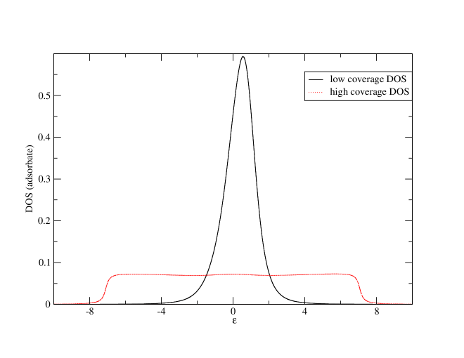
Figure 1: Comparison of density of states of the adsorbate for weakly coupled regime at low ($\theta$ = 0.1) and high coverage factor ($\theta$ = 0.9). he values of parameters (in eV) are as follows: $E^{r}_{r}=0.6,E^{r}_{ar}(0)=0.2,E^{r}_{a}=0.4$ and $v$ = 0.5 eV.

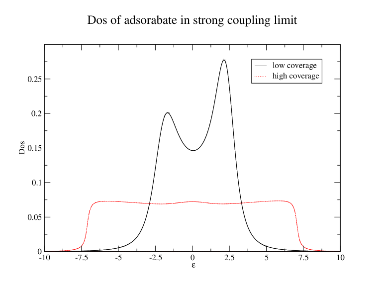
Figure 2: Comparison of density of states of adsorbates for strong coupling regime at low and high coverage factor. The values of the various parameters employed (in eV) are as follows: $E^{r}_{r}=1.0,E^{r}_{ar}(0)=0.25,E^{r}_{a}(0)=0.75,\Delta_{||}=1.5,\Delta_{\perp}=1.5,\mu=4.5,\upsilon=2.0$

In what follows, we describe the current vs overpotential profile for different sets of parameters. The adsorbate-electrode interaction is treated both in the weak ($v=0.5eV$) and strong ($v=2.0eV)$ coupling limits. When the coverage is low, the adsorbate density of states has a single peak Fig. 1 . An important consequence of the strong coupling limit is the splitting of the adsorbate level in bonding and anti-bonding states for low $\theta$ Fig.2. This feature is recaptured in the present analysis since energy dependence of $\Delta(\epsilon)$ is explicitly treated in the present approach (Eqs  A-14,  A-15). On the other hand, the well known wide-band approximation for $\Delta(\epsilon)$ fails to provide the bonding anti-bonding splitting. In the monolayer regime, due to the 2-d bond formation by the adsorbate layer, its density of states acquires a flat profile, irrespective of the strength of the electrode-adsorbate coupling (Fig  1,  2) . The table I summarizes the values of parameters used in the calculations.

Table 1: Values of parameters used in calculation in eV

	$v$	$\Delta_{||}$	$\Delta_{\perp}$	$\mu$	$E_{r}$	$E_{ar}$ (0)	$E_{a}$ (0)
strong	2.0	0.75	1.5	4.5	1.0	0.25	0.75
weak	0.5	0.75	1.5	4.5	0.6	0.2	0.4

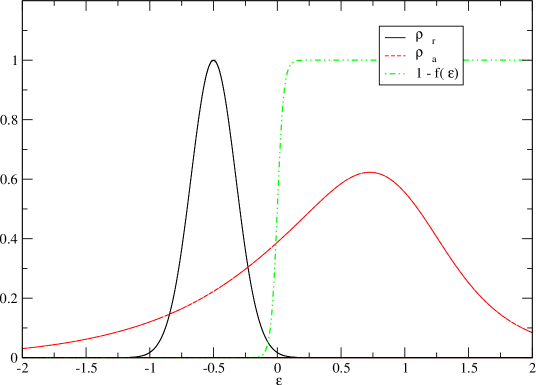
Figure 3: Plots showing the density of states for redox, adsorbate and the Fermi distribution for anodic current under zero overpotential. The weakly coupled regime and low coverage of $\theta$ = 0.3 is considered here .The values of parameters (in eV) are as follows: $E^{r}_{r}=0.6,E^{r}_{ar}(0)=0.2,E^{r}_{a}=0.4$ and $v$ = 0.5 eV .

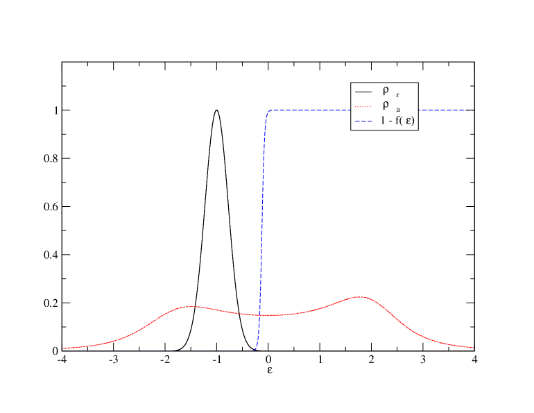
Figure 5: Plots showing the density of states for redox, adsorbate and the Fermi distribution for anodic current under zero overpotential. The strongly coupled regime and low coverage of $\theta$ = 0.3 is considered here .The values of parameters (in eV) are as follows: $E^{r}_{r}=1.0,E^{r}_{ar}(0)=0.25,E^{r}_{a}=0.75$ and $v$ = 2.0 eV .

Ideally, under zero overpotential condition, the anodic and cathodic currents are expected to be equal in magnitude. This implies that the profile of the product $\rho_{r}^{an}(\epsilon)*\rho_{a}^{an}(\epsilon)$ for anodic current is identical to the product profile $\rho_{r}^{cat}(\epsilon)*\rho_{a}^{cat}(\epsilon)$ for the cathodic current. This is a consequence of equal separation between the peak positions of adsorbate and reactant density of states for anodic and cathodic processes during equlibrium. [Fig. 3, 4]. The corresponding plots for strongly coupled regime is also shown in Fig. 5, 6

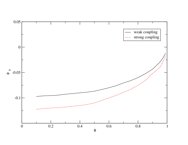
Figure 7: Plots showing the variation of $\Delta\phi$ with respect to $\theta$ the coverage factor. The values of re-organisation energies employed were same in both the curves. $E_{r}$ = 0.6 eV, $E_{a}(0)$ = 0.4 eV, $E_{ar}(0)$ = 0.2 eV

As noted earlier, the electrochemical potential $\mu$ has been set as the zero of energy scale for the direct electron transfer reaction. The presence of additional charge particles for the bridge assisted electron transfer reaction, namely the adsorbates, changes the equilibrium potential of the electrode. This is turn gets reflected as a $\theta$ dependent variation $\Delta\phi(\theta)$ in $\mu(\equiv 0)$. The fact that the anodic and cathodic currents at equilibrium potential are identical in magnitude provides a novel method for the determination of $\Delta\phi(\theta)$. Thus the relation $I_{a}(\eta=0)=I_{c}(\eta=0)$ with $f(\epsilon)={\bf(1+exp(-\beta(\epsilon+\Delta\phi(\theta)))^{-1}}$ { } (cf eqs.  6 and  22) enables us to evaluate $\Delta\phi(\theta)$. The variation of $\Delta\phi$ with respect to $\theta$ is shown in Fig.7 in the limit of weak and strong adsorbate-electrode interaction, with $E^{r}_{r}$ = 0.6 eV, $E^{r}_{ar}$(0) = 0.2 eV, $E^{r}_{a}$ (0) = 0.4 eV. The value of $\Delta\phi(\theta)$ depends on the strength of coupling $v$; its magnitude increases as the coupling becomes stronger. $|\Delta\phi(\theta)|$ is again large for low $\theta$ values and remains almost constant in this region. Note that in this regime, the charge on the adsorbate remains localized on the adsorption site. $|\Delta\phi(\theta)|$ starts diminishing sharply for $\theta>0.6$ and it tends to 0 as $\theta\rightarrow 1$. This behaviour is expected. As $\theta\rightarrow 1$, the adsorbate layer becomes metallic and gets incorporated in the electrode. The electron transfer acquires the characteristics of a direct heterogeneous reaction, and consequently as noted earlier, the electrochemical potential $\mu$ again lies at the zero of the energy scale.

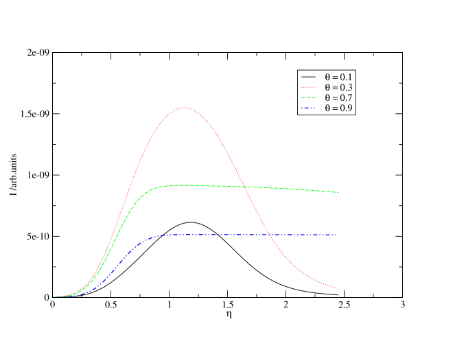
Figure 8: anodic current vs $\eta$ for $\alpha$ = 0.3. The values of the various parameters employed (in eV) are as follows: $E^{r}_{r}=1.0,E^{r}_{ar}(0)=0.25,E^{r}_{a}(0)=0.75,\Delta_{||}=1.5,\Delta_{\perp}=1.5,\mu=4.5,\upsilon=2.0$

We first present the current-overpotential profile in the weak coupling limit ($v=0.5~{}eV$) for a range of $\theta$ and $\alpha$. The employed values of various reorganization energies are $E^{r}_{r}$ = 0.6, $E^{r}_{ar}$(0) = 0.2, $E^{r}_{a}$ (0) = 0.4. The general behaviour can be analysed by looking at the case of lower coverage and high coverage regimes respectively, and then by investigating the effect of variation of $\alpha$ in these limits. Fig. 8 shows that for a fixed $\alpha$, anodic current as well as the current peak height increases with $\theta$ in the small $\theta$ range (curve a and b). This feature arises due to a better overlap between the reactant and adsorbate density of states, whose peak positions are approximately separated by a distance $E_{r}^{r}+E_{a}^{r}(\theta)-E_{ar}^{r}(\theta)$. An increase in $\theta$ reduces $E_{a}^{r}$ and $E_{ar}^{r}$ (cf eq.  25), and hence the peak separation diminishes and the overlap gets enhanced. The presence of anodic current peak at $\eta_{p}$ signifies negative differential resistance for $\eta>\eta_{p}$. This feature is absent in the higher coverage limit. For large value of $\theta$, the current at higher $\eta$ exhibits a saturation effect. This is a consequence of the fact that the maximum n in the adsorbate density of states $\rho^{an}_{a}$ is now absent. $\rho^{an}_{a}$ now acquires a plateau profile (Fig 1). The plateau height, and therefore the overlap between the reactant and adsorbate density of states decreases with the increasing coverage . Therefore a decrease in the saturation current results as $\theta\rightarrow 1$ (curve $\theta$ = 0.7 and 0.9 in Fig. 8).

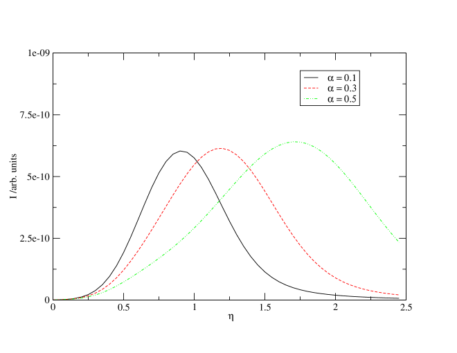
Figure 9: anodic current vs $\eta$ for $\theta$ = 0.1 in the weak coupled regime. The values of parameters (in eV) are as follows: $E^{r}_{r}=0.6,E^{r}_{ar}(0)=0.2,E^{r}_{a}=0.4$ and $v$ = 0.5 eV.

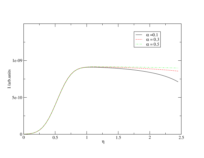
Figure 11: anodic current vs $\eta$ for $\theta$ = 0.7. The values of parameters (in eV) are as follows: $E^{r}_{r}=0.6,E^{r}_{ar}(0)=0.2,E^{r}_{a}=0.4$ and $v$ = 0.5 eV.

The effect of the $\alpha$ variation on the anodic current is highlighted in Fig. 9, 10 and  11 The effect is more pronounced in the low coverage regime due to the presence of adsorbate density of states peak. The reactant and adsorbate density of states peak separation increases with the increasing $\alpha$. Consequently, the maximum overlap between the two occurs at larger $\eta$. This explains the occurrence of the anodic current peak at higher $\eta$ values as $\alpha$ increases . On the other hand, the near constant adsorbate density of states for large $\theta$ ensures a minimal effect of $\alpha$ variation on the anodic current (Fig. 11, 12).

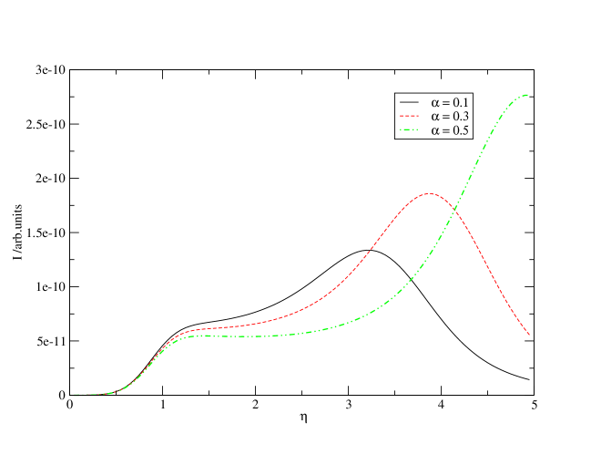
Figure 13: anodic current vs $\eta$ for $\theta=0.1$. The values of the various parameters employed (in eV) are as follows: $E^{r}_{r}=1.0,E^{r}_{ar}(0)=0.25,E^{r}_{a}(0)=0.75,\Delta_{||}=1.5,\Delta_{\perp}=1.5,\mu=4.5,\upsilon=2.0$

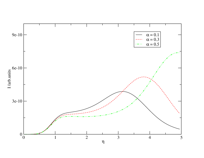
Figure 14: anodic current vs $\eta$ for $\theta=0.3$.The values of the various parameters employed (in eV) are as follows: $E^{r}_{r}=1.0,E^{r}_{ar}(0)=0.25,E^{r}_{a}(0)=0.75,\Delta_{||}=1.5,\Delta_{\perp}=1.5,\mu=4.5,\upsilon=2.0$

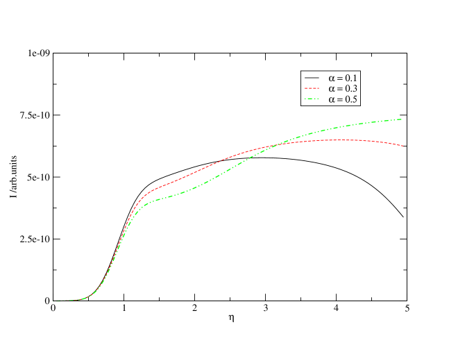
Figure 15: anodic current vs $\eta$ for $\theta=0.7$. The values of the various parameters employed (in eV) are as follows: $E^{r}_{r}=1.0,E^{r}_{ar}(0)=0.25,E^{r}_{a}(0)=0.75,\Delta_{||}=1.5,\Delta_{\perp}=1.5,\mu=4.5,\upsilon=2.0$

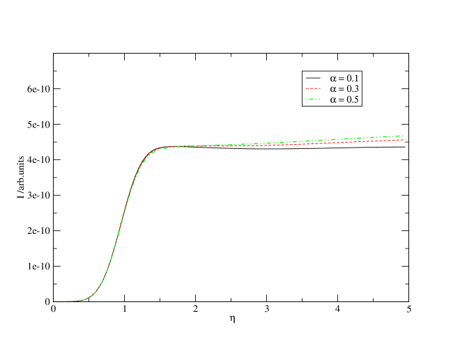
Figure 16: anodic current vs $\eta$ for $\theta=0.9$. The values of the various parameters employed (in eV) are as follows: $E^{r}_{r}=1.0,E^{r}_{ar}(0)=0.25,E^{r}_{a}(0)=0.75,\Delta_{||}=1.5,\Delta_{\perp}=1.5,\mu=4.5,\upsilon=2.0$

Next the strong coupling limit with [$v$ = 2.0 eV, $E^{r}_{r}$ = 1.0, $E^{r}_{ar}$(0) = 0.25, $E^{r}_{a}$ (0) = 0.75 ]is considered. Figures 13,14,15 and 16 shows the current overpotential response in the strong coupling regime. As in the case of low coverage, the $I_{a}$ vrs $\eta$ plot exhibits a negative-differentail region (Fig. 13, 14).

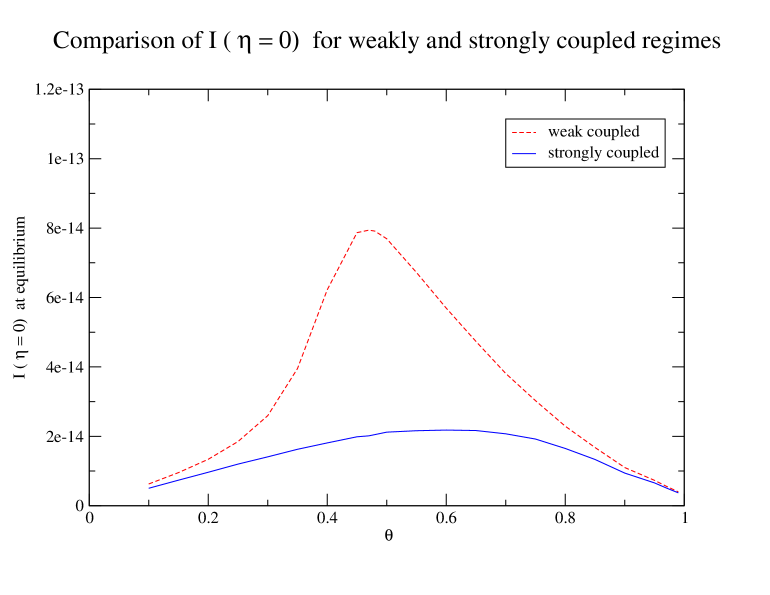
Figure 17: Plots showing the equilibrium current at zero overpotential $I_{0}$ vs $\theta$ for strong and weak coupled regime. The values of re-organisation energies were selected be the same for both the curves, $E_{r}$ = 0.6 eV, $E_{a}(0)$ = 0.4 eV, $E_{ar}(0)$ = 0.2 eV

More importantly, the presence of two peaks in $\rho_{a}^{an}$ when coupling $v$ is large and $\theta$ is small (Fig. 2) leads to a saddle point and a maximum in the $I_{a}$ vrs. $\eta$ plot. For the set of parameters currently employed, the $I_{A,Max}$ now occurs at a much larger $\eta$ in comparison to the weak coupling limit, and may not be accessible experimentally. However, the saddle point in the current appears in an overpotential range where the anodic current peak appears in the weak coupling limit. For large coverage, current potential profile are similar in strong and weak coupling limit. Interestingly, the saturation current is smaller in the large coupling case due to a decrease in the height of $\rho^{an}_{a}$. In fact this lowering of the current in the strong coupling is holds true for any coverage and $\eta$. This is shown in Fig. 17 wherein the variation of equilibrium current $I^{o}$ with respect to coverage is plotted The $I^{o}$ is smaller for larger $v$, and as explained earlier in the context of Fig. 8, shows a maximum in the intermediate coverage regime. However it may be noted that when $v\rightarrow 0$, current would be proportional to $|v|^{2}$, and an increase in $v$ in this very weak coupling limit will lead to an increase in the current.

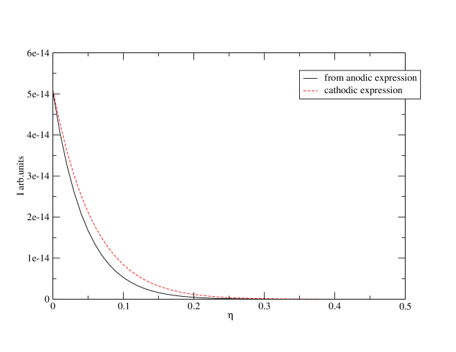
Figure 18: Comparison of cathodic current obtained from corresponding expression for cathodic current and from empirical relation of anodic current, $I_{c}=exp[-\beta\eta]I_{a}$. The specific case selected is for $\theta$ = 0.1 and $\alpha$ = 0.5 in the weakly coupled regime. The values of parameters (in eV) are as follows: $E^{r}_{r}=0.6,E^{r}_{ar}(0)=0.2,E^{r}_{a}=0.4$ and $v$ = 0.5 eV.

The results presented till now correspond to anodic current. But the formalism developed here also yields the cathodic current. In fact the equivalence of anodic and cathodic currents at the equilibrium potential has been earlier employed to determine the the variation in the equilibrium potential due to varying adsorbate coverage. The dependence of the cathodic current $I_{c}$ on overpotential $\eta$ is plotted in Fig. (18). It is often presumed that $I_{c}=e^{-\eta}I_{a}$ (Fig. 18). The present ‘microscopic’ calculations show that it is not entirely true. The calculated current value is slightly larger than the $e^{-\eta}I_{a}$ when $\eta<$ 0.

The high coverage regime of $\theta\rightarrow 1$ corresponding to a formation of monolayer of A decrease in the current for higher $\eta$ when the coverage is low virtually mimics the Marcus inverted region for a homogeneous electron transfer reaction. On the other hand, the current getting saturated at higher $\eta$ when the coverage is large is also true for a direct heterogeneous electron transfer reaction. Thus depending on the extent of coverage, an adsorbate mediated electron transfer at an electrode exhibits the characteristics of both homogeneous and heterogeneous electron transfer reactions. The localization of adsorbate electron at low coverage and its delocalization at high coverage is the reason behind this phenomena.

4 Summary and Conclusions

In this work, we considered electron transfer in an electrochemical system, from a solvated redox to an electrode mediate by intervening adsorbate atoms. Further randomness is introduced in the model in terms of the coverage factor which relates to the number of adsorbate atoms adsorbed on the electrode surface. The theory developed is valid for a range of regime, lone adsorbate mediate transfer to the monolayer formated direct electron transfer regime. The inherent randomness involved in the adsorbate distribution on the surface has been tackled by coherent potential approximation (CPA) and separate expression are derived for anodic and cathodic current.

Explicit attention was paid to the low coverage and high coverage regime, even though the formalism is valid for all regime, since at these two regions the theory could be compared with pre-existing literature. Plots were also provided for intermediate regimes and additionally, the effect of the adsorbed atoms on the Fermi level of the electrode were incorporated by means of a shifted potential $\Delta\phi(\theta)$, ensuring that the anodic and cathodic current were equal under zero overpotential condition.

The analysis also provides a novel method for determining the variation in $\Delta\phi(\theta)$ with changing adsorbate coverage.

The fraction of overpotential drop across the electrode-adsorbate is incorporated and the collective plots are analysed. We have proved that this fraction of overpotential drop plays a significant role in determining the response behaviour of current, typically the location and extent of the maximas in case of lower coverage situations. while in case of high coverage regime, the effect is not profound and the electron transfer follows the traditional direct electron transfer as expected from heuristic arguments.

The dependence of anodic current in the weak and strong electrode-adsorbate coupling is analyzed. In the former case, $I_{a}$ vrs overpotential profile exhibits a peak, where as in the later case, and in the same overpotential region, the current plot shows a saddle point behaviour. This fact can be used to distinguish a weakly chemisorbed bridge from a strongly chemisorbed one. These distinguishing features occur only when the coverage is low. At high coverage, $I_{a}\sim\eta$ plots have identical profile for weak and strong coupling cases

The calculated cathodic current gives a slightly higher value of $I_{c}$ in comparison to a presumed $I_{c}$ which equals $e^{-\eta}I_{a}$.

At low coverage, it is possible to recover the Marcus inverted region, which is absent when the coverage is large. The localized nature of the adsorbate orbital when coverage is low, and its getting delocalised for high coverages leads to this behaviour.

appendix

The microscopic current associated with the electron transfer reaction depends on the average value of the rate of change of electronic occupancy of the redox orbital [ ]

$$I=-e\left<\frac{\displaystyle\partial n_{r}}{\displaystyle\partial r}\right>$$ (A-1)

Treating $v_{ar}$ as a small quantity, a linear response formalism can be used to evaluate $<\dot{n}_{r}>$. Consequently,

$$I\ =\ \frac{e}{\hbar^{2}}\sum_{\sigma}\int^{\infty}_{-\infty}<[V^{\dagger}_{I\sigma}(0),V_{I\sigma}(t)]_{-}>dt$$ (A-2)

where

$$V_{I\sigma}\ =\ v_{ar}C_{a\sigma}^{\dagger}C_{r}$$ (A-3)

The first term in the commutator leads to anodic and the second one gives the cathodic current. The expectation value in (A-2) now corresponds to a density matrix defined for the Hamiltonian $H^{\prime}=H-\sum_{\sigma}(V^{\dagger}_{Ir}+V_{Ir})$. $H^{\prime}$ also determines the time evolution of various operators in (A-2). Employing the Frank-Condon approximation and treating the low frequency polarization modes in the semi-classical approximation, anodic current is obtained as

$$I_{a}\ =\ \frac{e}{\hbar}^{2}\int^{\infty}_{-\infty}dt|V_{at}|^{2}<<C^{\dagger}_{r}(0)C_{r}(t)>_{F}<C_{a\sigma}(0)C^{\dagger}_{a\sigma}(t)>_{F}>_{B}$$ (A-4)

where

$$<c^{\dagger}_{r}(0)c_{r}(\tau)>_{F}\ =\ \frac{\displaystyle 1}{\displaystyle\pi}\int^{\infty}_{-\infty}e^{-i\epsilon\tau/{\hbar}}\delta(\epsilon-\epsilon_{r})d\epsilon$$ (A-5)

The time correlation function involving $c_{a},~{}c^{\dagger}_{a}$ can be expressed in terms of adsorbate Green’s function

$$<c_{a\sigma}(0)c^{\dagger}_{a\sigma}(t)>_{F}\ =\ \frac{\displaystyle 1}{\displaystyle\pi}\int^{\infty}_{-\infty}(1-f(\epsilon))e^{i\epsilon\tau/{\hbar}}(ImG_{ii})_{i=a}d\epsilon$$ (A-6)

where

$$(G_{ii}(\epsilon))_{i=a}\ =\ <0|c_{a\sigma}<\frac{\displaystyle 1}{\displaystyle\epsilon-H^{\prime}}>_{c,i=a}c^{\dagger}_{a\sigma}|0>_{F}$$ (A-7)

Here $<...>_{F}$ implies an average over electronic degrees of freedom, keeping bosonic variables as fixed parameters. $<...>_{B}$ denotes the thermal average over boson modes. $<...>_{c,i=a}$ denotes a restricted configuration average. It implies that while obtaining the configuration average, the site a, which is occupied by an adsorbate and through which the electron transfer takes place, is excluded from the averaging. The occupancy status of the remaining sites are still unspecified. We replace the random medium encompassing the remaining sites by an effective medium using the CPA technique. The picture which now emerges is the one in which a reactant is coupled to an adsorbate occupying the site a, and this particular adsorbate is embedded in a two dimensional effective medium.

The randomness associated with these sites can be handled using the coherent potential approximation [ ]. Accordingly, the random energy operator $\hat{\epsilon}_{i\sigma}(<q_{\nu}>)n_{n\sigma}$ in eq.  4 is now replaced by a deterministic operator $k_{\sigma}n_{i\sigma}$. The coherent potential $k_{\sigma}(\epsilon,<q_{\nu}>)$ is same for all the sites, but depends on the energy variable $\epsilon$. $k_{\sigma}$ is determined self-consistently through the expression [ ]

$$\bar{G}_{ii}\ =\ \frac{1}{N_{||}}\sum_{u}\frac{1}{\epsilon-k_{\sigma}(\epsilon,<q_{\nu}>)-\epsilon_{u}-W^{\prime}(\epsilon,u)}\ =\ \frac{1-\theta}{\epsilon_{a\sigma}-k_{\sigma}(\epsilon,<q_{\nu}>)}$$ (A-8)

where 2D adsorbate lattice has $N_{||}$ number of sites, and

$$\begin{array}[]{lcl}W(\epsilon,u)&=&\sum_{j}e^{i{\bf u}.{\bf R}_{ji}}[v_{ij}+W^{\prime}_{ij}(\epsilon)]\\ \\ &=&\epsilon_{u}+\sum_{j}e^{i{\bf u}.{\bf R}_{ji}}W^{\prime}_{ij}(\epsilon)\\ \\ &=&\epsilon_{u}+W^{\prime}(\epsilon,u)\end{array}$$ (A-9)

The $(G_{ii})_{i=a}$ can be related to the complete configuration averaged GF $\bar{G_{ii}}$

$$(G_{ii})_{i=a}\ =\ \bar{G_{ii}}(\epsilon)[1-(\hat{\epsilon}_{a\sigma}(q_{\nu})-k_{\sigma}(\epsilon))\bar{G}_{ii}(\epsilon)]^{-1}$$ (A-10)

The tedious summation over the momentum k of metal states and the momentum u of the Bloch states in 2D adsorbate layer, commensurate with the underlying electrode surface lattice, can be considerably simplified under the following assumptions. (i) The separability of the metal state energy $\epsilon_{k}$ in the direction parallel and perpendicular to the surface. (ii) The substrate density of states in the direction perpendicular to surface is taken to be Lorentzian, whereas the same is assumed to be rectangular along the surface. (iii) The adsorbate occupies the ‘on-top’ position on the electrode, and is predominantly coupled to the underlying substrate atom with coupling strength $v$. Consequently, eq.(A9) now becomes

$$\begin{array}[]{lcl}\bar{G}_{ii}(\epsilon)&=&\frac{\displaystyle 1-\theta}{\displaystyle\epsilon_{a\sigma}\{<q_{\nu}>\}-k_{\sigma}\{\epsilon,<q_{\nu}>\}}\\ \\ &=&\frac{\displaystyle 1}{\displaystyle 2\Delta_{||}(B-A)\mu}\left[(A-C)\ln\left(\frac{A-\Delta_{||}}{A+\Delta_{||}}\right)-(B-C)\ln\left(\frac{B-\Delta_{||}}{B+\Delta_{||}}\right)\right]\end{array}$$ (A-11)

with

$$A/B\ =\ \frac{1}{2}[(C+D)\pm\{(C+D)^{2}-4(CD-\frac{v^{2}}{\mu})\}^{\frac{1}{2}}]$$ (A-12)

$$C\ =\ \frac{\epsilon-k_{\sigma}\{\epsilon,<q_{\nu}>\}}{\mu}\quad;\quad\ D\ =\ \epsilon-i\Delta_{\perp};\quad\mu\ =\ \theta\delta/\Delta_{||}$$ (A-13)

$\delta$ is the half-bandwidth of adsorbate monolayer and $\mu$ is the same for an arbitrary coverage $\theta$. $2\Delta_{||}$ is the substrate bandwidth at the surface and $\Delta_{t}$ the total bandwidth of the substrate $2(\Delta_{||}+\Delta_{\perp})=\Delta_{t}$.

$$\frac{1}{N_{\perp}}\sum\delta(\epsilon-\epsilon_{k_{z}})=\frac{1}{\pi}\frac{\Delta_{\perp}}{(\epsilon-\epsilon_{k_{z}})^{2}+\Delta_{\perp}^{2}}$$ (A-14)

$$\frac{1}{N_{||}}\sum\delta(\epsilon-\epsilon_{u})=1/2\Delta_{||}\quad;\quad-\epsilon<\Delta_{||}<\epsilon$$ (A-15)

Where the separability of metal states energies ${\epsilon_{k}}$ in directions parallel and perpendicular to the surface is a crucial assumption made here. $\epsilon_{k}=\epsilon_{u}+\epsilon_{k_{z}}$.

The self-consistent value of $k_{\sigma}(\epsilon)$ is obtained from eq. A-11, which also determines $\bar{G}_{ii}$.

Expressing

$$\bar{G}^{-1}_{ii}+K_{\sigma}\{\epsilon,<q_{\nu}>\}\ =\ X_{1}(\epsilon,\theta)+i~{}sgn(X_{2}(\epsilon,\theta))|X_{2}(\epsilon,\theta)|$$ (A-16)

enables us to write (cf. eq.(A11))

$$Im(G_{ii})_{i=a}\ =\ -sgn(X_{2})\frac{\displaystyle|X_{2}|}{\displaystyle(X_{1}(\epsilon,\theta)-\hat{\epsilon}_{a\sigma}(q_{\nu}))^{2}+X^{2}_{2}}$$ (A-17)

where sgn$(X)$ = +1 when $X>0$ and -1 otherwise.

To evaluate the anodic current $I_{a}$, one finally needs to carry out the thermal average over low frequency boson modes. The required density matrix for this average in the semi-classical limit is

$$P(q_{\nu})\ =\ W(q_{\nu})/\int^{\infty}_{-\infty}W(q_{\nu})dq_{\nu}$$ (A-18)

$$W(q_{\nu})\ =\ exp[-\beta\sum_{\nu=1,2}\frac{\omega_{\nu}}{2}(p_{\nu}^{2}+q_{\nu}^{2})+\bar{\lambda}_{\nu}q_{\nu}]$$ (A-19)

With the above defined probability function the net expression for anodic current is shown below

$$I_{a} = e\langle n_{r}\rangle\mid\upsilon_{ar}\mid^{2}\frac{1}{\sqrt{\pi}\hbar}\frac{1}{\mathrm{Z}}\int d\epsilon\int(\Pi_{\nu}dq_{\nu})\int dt\int d\tau[(1-f(\epsilon)]$$ (A-20)

$$exp[-\beta\sum_{\nu=1,2}\frac{\omega_{\nu}}{2}(p_{\nu}^{2}+q_{\nu}^{2})+\bar{\lambda}_{\nu}q_{\nu}]\quad exp[i(\epsilon-\epsilon_{r}-\sum_{\nu}\lambda_{r\nu}q_{\nu})t]$$

$$exp[i(X_{1}(\epsilon,\theta)-\epsilon_{a}-\sum_{\nu}\lambda_{a\nu}q_{\nu})\tau-\mid X_{2}(\epsilon,\theta)\mid\mid\tau\mid]$$

where $\mathrm{Z}=\int(\Pi_{\nu}dq_{\nu})exp[-\beta\sum_{\nu}\frac{\omega_{\nu}}{2}(p_{\nu}^{2}+q_{\nu}^{2})+\bar{\lambda}_{\nu}q_{\nu}]$ The expression for cathodic current has a similar form with the $1-f(\epsilon)$ replaced by $f(\epsilon)$ and $\bar{\lambda}_{\nu}$ defined accordingly. For anodic current $\bar{\lambda}_{\nu}=\lambda_{c\nu}+\lambda_{o\nu}+\lambda_{r\nu}$, while for cathodic current, $\bar{\lambda}_{\nu}=\lambda_{c\nu}+\lambda_{o\nu}+\lambda_{a\nu}$. Carrying out the various integrations leads to the result employed in the main article.

$$I_{a}=e\langle n_{r}\rangle\mid\upsilon_{ar}\mid^{2}\frac{1}{\sqrt{\pi}\hbar}\int d\epsilon(1-f(\epsilon))\rho_{a}(\epsilon)\frac{\mathrm{Re}\omega_{z}}{2\sqrt{\pi\mathrm{P}}}$$ (A-21)

Figures

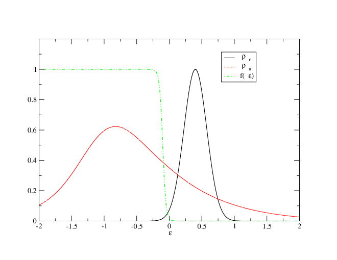
Figure 4: Plots showing the density of states for redox, adsorbate and Fermi distribution for cathodic current at zero overpotential. The values of parameters are same as in 3

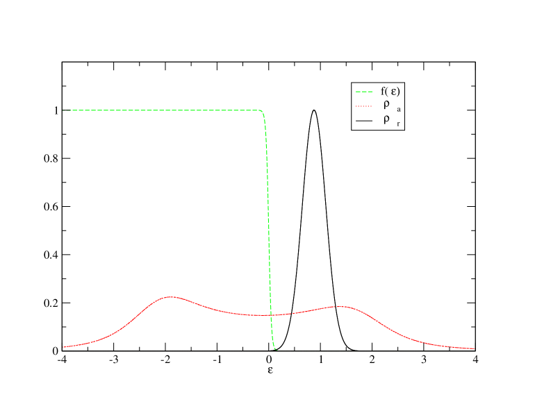
Figure 6: Plots showing the density of states for redox, adsorbate and Fermi distribution for cathodic current at zero overpotential. The values of parameters are same as in 5

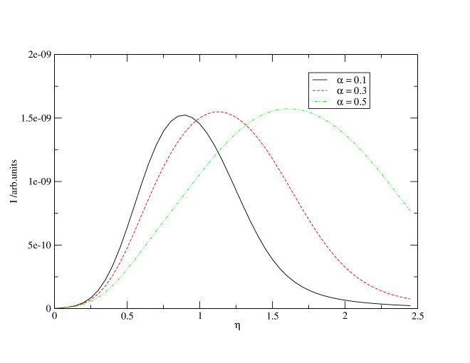
Figure 10: anodic current vs $\eta$ for $\theta$ = 0.3 in weak coupled regime. The values of parameters (in eV) are as follows: $E^{r}_{r}=0.6,E^{r}_{ar}(0)=0.2,E^{r}_{a}=0.4$ and $v$ = 0.5 eV.

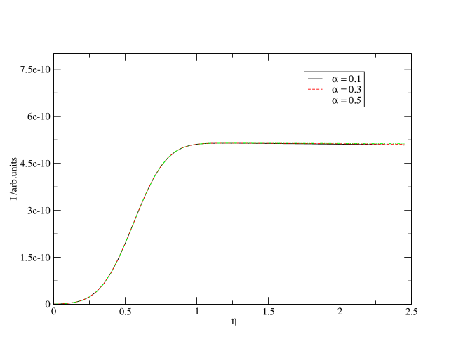
Figure 12: anodic current vs $\eta$ for $\theta$ = 0.9. The values of parameters (in eV) are as follows: $E^{r}_{r}=0.6,E^{r}_{ar}(0)=0.2,E^{r}_{a}=0.4$ and $v$ = 0.5 eV.

References

- [1] R.A. Drust, A.J. Baumner, R.W. Murray, R.P. Buck, and C.P. Andrieux, Pure and Appl. Chem. 69, 1317 (1997).
- [2] R. M. Metzger, T. Xu and I. R. Peterson, J. Chem. Phys. B. 105 7280 (2001).
- [3] A. Salomon, D. Cahen, S. M. Lindsay, J. Tomfohr, V. B. Engelkes and C. D. Frisbie, Adv. Mater. 15 1881 (2003).
- [4] In Electron Transfer from Isolated Molecules to BioMolecules; 106, J. Jortner and M. Bixon, Eds, wiley; New York, 1999.
- [5] In Electron and Proton Transfer in Chemistry and Biology; A. Muller, Eds, Elsevier; Amsterdam, 1992.
- [6] M. A. Reed et. al, Science, 278, 252 (1997).
- [7] C. Joachim et. al Phys. Rev. Lett 74, 2101 (1995).
- [8] In Atomic and Molecular Wires, C. Joachim and S. Roth, Eds, kluwer Academy; Dordrecht, 1997.
- [9] F. Remacle and R. D. Levine, Faraday Discussions, 131 45 (2006).
- [10] S. M. Lindsay, Faraday Discussions, 131 403 (2006).
- [11] A. K. Mishra, J. Phys. Chem. B. 103, 1484 (1999).
- [12] A. K. Mishra, R. Kishore and W. Schmickler, J. Electroanal. Chem. 574 1 (2004).
- [13] A. K. Mishra and W. Schmickler, J. Chem. Phys. 121 1020 (2004).
- [14] J. Neugebauer and M. Scheffler, Phys. Rev. B, 46 16067 (1992).
- [15] J. Neugebauer and M. Scheffler, Phys. Rev. Lett, 71 577 (1993).
- [16] H. Over et. al, Surf. Sci. Lett, 2 409 (1995).
- [17] J. Bormet et. al, Phys. Rev. B, 49 17242 (1994).
- [18] J. Bormet et. al, Comput. Phys. Commun. 107 187 (1994).