Existence of the excitonic insulator phase in the extended Falicov-Kimball model: an $SO(2)$-invariant slave-boson approach

Abstract

We re-examine the three-dimensional spinless Falicov-Kimball model with dispersive $f$ electrons at half-filling, addressing the dispute about the formation of an excitonic condensate, which is closely related to the problem of electronic ferroelectricity. To this end, we work out a slave-boson functional integral representation of the suchlike extended Falicov-Kimball model that preserves the $SO(2)\otimes U(1)^{\otimes 2}$ invariance of the action. We find a spontaneous pairing of $c$ electrons with $f$ holes, building an excitonic insulator state at low temperatures, also for the case of initially non-degenerate orbitals. This is in contrast to recent predictions of scalar slave-boson mean-field theory but corroborates previous Hartree-Fock and RPA results. Our more precise treatment of correlation effects, however, leads to a substantial reduction of the critical temperature. The different behavior of the partial densities of states in the weak and strong inter-orbital Coulomb interaction regimes supports a BCS-BEC transition scenario.

I Introduction

The excitonic instability in solids is driven by the Coulomb attraction between electrons and holes which under certain conditions causes them to form bound states. At the semimetal-semiconductor transition the conventional ground state of the crystal may become unstable with respect to the spontaneous formation of excitons. Starting from a semimetal with a sufficiently small number of electrons and holes, such that the Coulomb interaction is basically unscreened, the number of free carriers will vary discontinuously under an applied perturbation Mott (1961), signaling a phase transition. Approaching the transition from the semiconductor side, an anomaly occurs when the (indirect) band gap, tuned, e.g., by external pressure, becomes less then the exciton binding energy Knox (1963). As a consequence, a new distorted phase of the crystal, with spontaneous coherence between conduction and valence bands and a gap for charged excitations, develops. It separates, below a critical temperature, the semimetal from the semiconductor. This state, known as ‘excitonic insulator’ (EI), can be regarded as an electron-hole pair (exciton) condensate Halperin and Rice (1967). By nature, depending on from which side of the semimetal-semiconductor transition the EI is approached, the EI typifies either as a BCS condensate of loosely bound electron-hole pairs or as a Bose-Einstein condensate (BEC) of preformed tightly-bound excitons Leggett (1980); Comte and Nozières (1982); Bronold and Fehske (2006).

The mean-field description of the EI phase is very similar to the BCS theory of superconductivity, and has been worked out long-time ago des Cloizeaux (1965); Kohn (1968); Keldysh and Kopaev (1965); Kozlov and Maksimov (1965); Jérome et al. (1967); Zittartz (1968). In this context also the transition from BCS to BE condensation was discussed Leggett (1980); Nozières and Schmitt-Rink (1985); Zimmermann and Stolz (1985); Kremp et al. (2008). Surprisingly enough, the quantitative semimetal-EI-semiconductor phase diagram has been determined only quite recently Bronold et al. (2007); Bronold and Fehske (2008); Kremp et al. (2008). All these investigations, having normal (excited) semiconductor systems in mind, rest on the standard effective-mass Mott-Wannier-type exciton model. Thereby important band-structure and correlation effects, as well as the exciton-excition and exciton-phonon interaction, and the inter-valley scattering of excitons were largely neglected.

In nature, the EI state is evidently rare. One obstacle for creating an excitonic condensate is the far-off-equilibrium situation caused by optical excitation of excitons. But also in thermal equilibrium situations, EI states are expected to occur only under very particular circumstances, e.g., if conduction and valence bands are adequately nested Bascones et al. (2002). Actual materials experimentally studied from the viewpoint of the EI are numbered. One recent example is quasi-one-dimensional $\rm Ta_{2}NiSe_{5}$ with highly polarizable Se, where angle-resolved photoemission spectra reveal an extreme valence-band top flattening indicating that the ground state might be viewed as an EI Wakisaka et al. (2009). At present, the transition-metal dichalcogenide $1T$-$\rm TiSe_{2}$ seems to be the only candidate for a low-temperature phase transition to the EI without the influence of any external parameters other than the temperature. Here the onset of an EI phase was invoked as driving force for the charge-density-wave transition Cercellier et al. (2007); Monney et al. (2009). Semiconducting, pressure-sensitive mixed valence materials, such as ${\rm TmSe_{0.45}Te_{0.55}}$, are further candidates for exciton condensation. Fine tuning the excitonic level to the narrow 4$f$ valence band, a rather large number of about $10^{20}-10^{21}$ $\rm cm^{-3}$ (small-to-intermediate sized) excitons can be created, which presumably condense into an EI state, at temperatures below 20 K in the pressure range between 5 and 11 kbar Neuenschwander and Wachter (1990); Bucher et al. (1991); Wachter et al. (2004). Clearly, for these rather complex transition-metal/rare-earth compounds with strong electronic correlations, simple effective-mass-model based theories will be too crude.

The investigation of Falicov-Kimball-type models offers another promising route towards the theoretical description of the EI scenario. In its original form, the Falicov-Kimball model Falicov and Kimball (1969); Ramirez et al. (1970) contains two types of fermions: localized $f$ electrons and itinerant $c$ electrons with orbital energies $E_{f}$ and $E_{c}$ , respectively. An on-site Coulomb interaction $U$ of both species determines the distribution of the electrons between the $f$ and $c$ sub-systems, and therefore may drive a valence transition, provided there is a way to establish $f$–$c$ coherence. At first glance this can only be achieved by including a hybridization of the $f$ and $c$ bands KMM76 ; Portengen et al. (1996a). It has been shown, however, that a finite $f$ bandwidth, being certainly more realistic than entirely localized $f$ electrons, will also induce $f$–$c$ transitions Batista (2002); Batista et al. (2004). The model with direct $c$–$c$ and $f$–$f$ hopping ($\propto t_{c/f}$), is sometimes called extended Falicov-Kimball model (EFKM), the Hamiltonian of which takes the form

$$H= E_{c}\sum_{i}c_{i}^{\dagger}c_{i}+t_{c}\sum_{\langle i,j\rangle}c_{i}^{\dagger}c_{j}+E_{f}\sum_{i}f_{i}^{\dagger}f_{i}+t_{f}\sum_{\langle i,j\rangle}f_{i}^{\dagger}f_{j}$$

$$+U\sum_{i}n_{ic}n_{if}\,.$$ (1)

Here $f_{i}^{\dagger}$ ($c_{i}^{\dagger}$) creates an $f$ ($c$) electron at lattice site $i$, and $n_{if}=f_{i}^{\dagger}f_{i}$ ($n_{ic}=c_{i}^{\dagger}c_{i}$) are the corresponding number operators. Let us emphasize that the $f$ and $c$ bands involved have different parity Batista (2002). For $t_{f}t_{c}<0$ ($t_{f}t_{c}>0$), we may have a direct (indirect) band gap. For $t_{f}\equiv 0$ (dispersionless $f$ band), the local $f$ electron number is strictly conserved Schneider and Czycholl (2008).

In the past few years, both the Falicov-Kimball model with hybridization KMM76 ; Portengen et al. (1996a, b); Czycholl (1999); Farkašovský (1999) and the EFKM Batista (2002); Batista et al. (2004); Farkašovský (2008); Schneider and Czycholl (2008) have been studied in connection with the exciting idea of electronic ferroelectricity. The origin of electronic ferroelectricity is a spontaneously broken symmetry due to a non-vanishing $\langle c^{\dagger}f\rangle$ average, which causes finite electrical polarizability without an external, interband-transition driving field. As $\langle c^{\dagger}f\rangle$ is basically an excitonic expectation value, indicating the pairing of $c$ electrons with $f$ holes, the problem of electronic ferroelectricity is intimately connected with the appearance of an excitonic condensate. Accordingly, the question whether the ground-state phase diagram of the EFKM exhibits an EI state has attracted much attention. By means of constrained path Monte Carlo (CPMC) techniques the $T=0$ phase diagram of the EFKM was determined in one and two dimensions in the strong and intermediate-coupling regimes Batista (2002); Batista et al. (2004). In both cases a ferroelectric phase was detected. A subsequent Hartree-Fock calculation shows that the mean-field phase diagram of the two-dimensional EFKM agrees even quantitatively with the CPMC data Farkašovský (2008), supporting the applicability of Hartree-Fock and RPA schemes to three- and infinite-dimensional systems Farkašovský (2008); Schneider and Czycholl (2008); Ihle et al. (2008). Surprisingly, the more sophisticated scalar slave-boson theory failed to find the EI phase when the $f$ and $c$ orbitals are non-degenerate Brydon (2008).

The continued controversy, regarding the existence of the EI phase in the EFKM, motivates us to re-examine the problem using an improved auxiliary boson approach that ensures the rotational and gauge symmetries of the EFKM within a functional integral scheme.

II Slave-Boson Theory

II.1 Slave-boson Hamiltonian

The extended Falicov-Kimball Hamiltonian (1) can be rewritten as an asymmetric Hubbard model if the orbital flavor $(f,c)$ is represented by a pseudo-spin variable $(\sigma=\uparrow,\downarrow)$. Using the spinor representation

$$\mathbf{a}_{i}=\left(\begin{matrix}a_{i\uparrow}\\ a_{i\downarrow}\end{matrix}\right)\,,\quad\mathbf{a}_{i}^{\dagger}=(a_{i\uparrow}^{\dagger},a_{i\downarrow}^{\dagger})\,,\quad\underline{t}=\left(\begin{matrix}\kappa&0\\ 0&1\end{matrix}\right)\,,$$ (2)

where the vectors $\mathbf{a}_{i}$ ($\mathbf{a}_{i}^{\dagger}$) are built up by the fermion annihilation (creation) operators $a_{i\uparrow}^{(\dagger)}\equiv f_{i}^{(\dagger)}$ and $a_{i\downarrow}^{(\dagger)}\equiv c_{i}^{(\dagger)}$, $H$ becomes

$$H=\sum_{i\sigma}E_{\sigma}a_{i\sigma}^{\dagger}a_{i\sigma}+\sum_{\langle i,j\rangle}\mathbf{a}_{i}^{\dagger}\;\underline{t}\;\mathbf{a}_{j}+U\sum_{i}n_{i\downarrow}n_{i\uparrow}\,.$$ (3)

In Eq. (2), $\kappa=t_{\uparrow}/t_{\downarrow}$ gives the ratio of the $f$- and $c$-bandwidths ($t_{\downarrow}=1$ fixes the unit of energy). Obviously, the usual Hubbard model follows for $E_{\uparrow}=E_{\downarrow}$ and $\kappa=1$. Without loss of generality we choose $E_{\downarrow}=0$ and $E_{\uparrow}\leq 0$ in what follows.

Now the slave-boson representation of the EFKM is constructed by replacing the fermionic Hilbert space by an enlarged one of pseudo-fermionic and bosonic states. The local states, representing the original physical states of the EFKM (1) in the enlarged Hilbert space in a one-to-one manner, can be created in the following way:

$$|0_{i}\rangle\;\;\rightarrow \;\;e_{i}^{\dagger}|\mathrm{vac}\rangle\,,$$ (4)

$$|2_{i}\rangle\;\;\rightarrow \;\;\tilde{a}_{i\uparrow}^{\dagger}\tilde{a}_{i\downarrow}^{\dagger}d_{i}^{\dagger}|\mathrm{vac}\rangle\,,$$ (5)

$$|\sigma_{i}\rangle\;\;\rightarrow \;\;\sum_{\rho}\tilde{a}_{i\rho}^{\dagger}p_{i\rho\sigma}^{\dagger}|\mathrm{vac}\rangle\,.$$ (6)

The pseudo-fermions $\tilde{a}_{i\rho}$ satisfy anti-commutation rules $\{\tilde{a}_{i\rho},\tilde{a}^{\dagger}_{j\rho^{\prime}}\}=\delta_{ij}\delta_{\rho\rho^{\prime}}$, while usual Bose commutation rules hold for the slave bosons: $[e_{i},e_{j}^{\dagger}]=\delta_{ij}$, $[p_{i\rho_{1}\rho_{2}},p^{\dagger}_{j\rho_{3}\rho_{4}}]=\frac{1}{2}\delta_{ij}\delta_{\rho_{1}\rho_{4}}\delta_{\rho_{2}\rho_{3}}$, and $[d_{i},d_{j}^{\dagger}]=\delta_{ij}$. The boson number operators, $e^{\dagger}_{i}e_{i}$, $2\,\mbox{Tr}\,{\underline{p}}^{\dagger}_{i}{\underline{p}}_{i}$, and $d^{\dagger}_{i}d_{i}$ project on an empty, a singly occupied and a doubly occupied state, respectively. By introducing a slave-boson matrix-operator for the case of single occupancy, $\underline{p}_{i}^{(\dagger)}$, we adapt the spin-rotation-invariant slave-boson formulation of the Hubbard model Li et al. (1989) (for a generalization to multi-orbital models see Lechermann et al. (2007)), in order to avoid difficulties that may arise from the scalar nature of the $p_{\sigma}$ bosons in approximative treatments Kotliar and Ruckenstein (1986); Brydon (2008). The decomposition

$$\underline{p}_{i}^{(\dagger)}=\frac{1}{2}\sum_{\mu=0}^{3}\underline{\tau}_{\mu}p_{i\mu}^{(\dagger)}$$ (7)

into scalar (singlet) $p_{i0}^{(\dagger)}$ and vector (triplet) $\vec{p}_{i}^{\,(\dagger)}=(p_{ix}^{(\dagger)},p_{iy}^{(\dagger)},p_{iz}^{(\dagger)})$ components, where $\underline{\tau}_{0}$ is the unity matrix and $\underline{\vec{\tau}}$ the vector of Pauli spin matrices, is given as

$$\underline{p}_{i}^{(\dagger)}= \frac{1}{2}\left(\begin{matrix}p_{i0}^{(\dagger)}+p_{iz}^{(\dagger)}&p_{ix}^{(\dagger)}-ip_{iy}^{(\dagger)}\\[2.84544pt] p_{ix}^{(\dagger)}+ip_{iy}^{(\dagger)}&p_{i0}^{(\dagger)}-p_{iz}^{(\dagger)}\end{matrix}\right)\,.$$ (8)

Of course, it is crucial to select out of the extended fermion-boson Fock space the physical states. This can be achieved by imposing two sets of local constraints:

$$C^{(1)}_{i} = e^{\dagger}_{i}e_{i}\;+2\,\mbox{Tr}\,{\underline{p}}^{\dagger}_{i}{\underline{p}}_{i}\,+d^{\dagger}_{i}d_{i}\,-1\,=0\,,$$ (9)

$$\underline{C}^{(2)}_{i} = \tilde{\mathbf{a}}_{i}\otimes\tilde{\mathbf{a}}^{\dagger}_{i}+2\,{\underline{p}}^{\dagger}_{i}{\underline{p}}_{i}+d^{\dagger}_{i}d_{i}\,\underline{\tau}_{0}-\underline{\tau}_{0}=0\,.$$ (10)

$C^{(1)}_{i}$ expresses the completeness of the bosonic operators, i.e. each lattice site $i$ can only be occupied by exactly one boson. $\underline{C}^{(2)}_{i}$ relates the pseudo-fermion number to the number of $\underline{p}$ and $d$ bosons.

Correspondingly, the mapping of the physical electron operators into products of new pseudo-fermions and slave bosons in the hopping term of $H$ is

$$\mathbf{a}_{i}\;\;\rightarrow \;\;\underline{z}_{i}\,\mathbf{\tilde{a}}_{i}\,.$$ (11)

The choice of the hopping operators $\underline{z}_{i}$ is not unique. This arbitrariness can be used, e.g., to reproduce, for the Hubbard model case, the correct free-fermion result at $U=0$ and the Gutzwiller result for any finite $U$ at the mean-field level, where the constraints (9) and (10) are fulfilled only on the average. This is guaranteed by choosing Li et al. (1989); Frésard and Wölfle (1992)

$${\underline{z}_{i}}={\underline{L}_{i}}e^{\dagger}_{i}{{M}_{i}}{\underline{p}_{i}}{\underline{N}_{i}}+{\underline{L}_{i}}{\tilde{\underline{p}}^{\dagger}_{i}}{{M}_{i}}d_{i}{\underline{N}_{i}}\;$$ (12)

with

$${\underline{L}}_{i} = [(1-d_{i}^{\dagger}d_{i})\underline{\tau}_{0}-2{\underline{p}}^{\dagger}_{i}{\underline{p}}_{i}]^{-1/2}\;,$$ (13)

$${\underline{N}_{i}} = [(1-e_{i}^{\dagger}e_{i})\underline{\tau}_{0}-2{\underline{\tilde{p}}}^{\dagger}_{i}{\underline{\tilde{p}}}_{i}]^{-1/2}\;,$$ (14)

$$M_{i} = [1+e^{\dagger}_{i}e_{i}+d^{\dagger}_{i}d_{i}+2\,\mathrm{Tr}\,{\underline{p}}^{\dagger}_{i}{\underline{p}}_{i}]^{1/2}\>,$$ (15)

and $\tilde{p}^{\left(\dagger\right)}_{i\rho\rho^{\prime}}=\rho\rho^{\prime}p^{\left(\dagger\right)}_{i-\rho^{\prime}-\rho}\;$. The Hubbard interaction term of $H$ can be bosonized via

$$n_{i\uparrow}n_{i\downarrow}\;\;\rightarrow \;\;d_{i}^{\dagger}d_{i}\,.$$ (16)

That is, the transformation to slave-boson fields results in a linearization of the interaction, and we end up with the EFKM Hamiltonian in the form

$$H=\frac{E_{\uparrow}}{2}\sum_{i}\mathbf{\tilde{a}}_{i}^{\dagger}(\underline{\tau}_{0}+\underline{\tau}_{z})\mathbf{\tilde{a}}_{i}+\sum_{\langle i,j\rangle}\mathbf{\tilde{a}}_{i}^{\dagger}\underline{z}_{i}^{\dagger}\,\underline{t}\,\underline{z}_{j}\mathbf{\tilde{a}}_{j}+U\sum_{i}d_{i}^{\dagger}d_{i}\,.$$ (17)

II.2 Functional integral representation

To proceed further, it is convenient to represent the grand canonical partition function of the constrained system (17), $Z=\mathrm{Tr}\,\mathrm{e}^{-\beta(H-\mu N_{e})}$, as an imaginary-time path integral over Grassmann fermionic and complex bosonic fields Negele and Orland (1988)

$$Z = \int D[\bar{\tilde{a}}_{\rho},\tilde{a}_{\rho}]\,D[e^{\ast},e]\,D[p^{\ast}_{\mu},p_{\mu}]\,D[d^{\ast},d]\,d[\lambda^{(1)}]\,d[\lambda^{(2)}_{\mu}]$$ (18)

$$\quad\quad\times\,\mathrm{e}^{-\int\limits_{0}^{\beta}\,d\tau L(\tau)}$$

with the Lagrangian

$$L(\tau) = \sum_{i}\Big{[}-\lambda^{(1)}_{i}+e^{\ast}_{i}(\partial_{\tau}+\lambda^{(1)}_{i})e_{i}$$ (19)

$$\quad\quad+2\,\mathrm{Tr}\,{\underline{p}^{\ast}_{i}}^{T}\big{(}(\partial_{\tau}+\lambda^{(1)}_{i})\underline{\tau}_{0}-{\underline{\lambda}^{(2)}_{i}}^{T}\big{)}{\underline{p}_{i}}^{T}$$

$$\quad\quad\quad\quad\quad+d^{\ast}_{i}(\partial_{\tau}+\lambda^{(1)}_{i}+U-\mathrm{Tr}\,{\underline{\lambda}^{(2)}_{i}})d_{i}\Big{]}$$

$$+\sum_{i}\mathbf{\bar{\tilde{a}}}_{i}\big{(}(\partial_{\tau}-\mu)\underline{\tau}_{0}+\underline{\lambda}_{i}^{(2)}+\tfrac{E_{\uparrow}}{2}(\underline{\tau}_{0}+\underline{\tau}_{z})\big{)}\mathbf{\tilde{a}}_{i}$$

$$+\sum_{\langle i,j\rangle}\mathbf{\bar{\tilde{a}}}_{i}\,\underline{z}_{i}^{\ast}\,\underline{t}\;\underline{z}_{j}\,\mathbf{\tilde{a}}_{j}\,.$$

Here $\beta=1/T$ is the inverse temperature and the time-independent Lagrange multipliers $\lambda_{i}^{(1)}$, $\underline{\lambda}_{i}^{(2)}=\lambda_{i0}^{(2)}\,\underline{\tau}_{0}+\vec{\lambda}_{i}^{(2)}\,\vec{\underline{\tau}}$ are introduced to enforce the constraints via the integral representation of the $\delta$-function Hooijer and Van Himbergen (1987),

$$\delta\big{[}C^{(l)}\big{]}=\frac{\beta}{2\pi i}\int\limits_{c}^{c+2\pi i/\beta}\;d\lambda^{(l)}\;e^{-\beta\lambda^{(l)}C^{(l)}}$$ (20)

(the path of the $\lambda$-integration is parallel to the imaginary axis and one finds $\lambda\in\mathbf{R}^{+}$ at the physical saddle point).

Next, exploiting the gauge symmetry of the action, we perform local time-dependent phase transformations:

$$e_{i} \rightarrow e_{i}\,e^{-i\vartheta_{i}}\,,$$ (21)

$$d_{i} \rightarrow d_{i}\,e^{-i\psi_{i}}\,,$$ (22)

$$\underline{p}_{i} \rightarrow\underline{p}_{i}\,e^{-i(\chi_{i0}\underline{\tau}_{0}-\chi_{iz}\underline{\tau}_{z})}\,,$$ (23)

$$\mathbf{\tilde{a}}_{i} \rightarrow\mathbf{\tilde{a}}_{i}\,e^{-i(\varphi_{i0}\underline{\tau}_{0}-\varphi_{iz}\underline{\tau}_{z})}\,.$$ (24)

Note that both the original as well as the transformed Bose fields are complex. By the transformation (24) the kinetic contribution generates extra terms violating the $SO(2)\otimes U(1)^{\otimes 3}$ invariance of the model. Transforming the Lagrange multipliers into real time-dependent Bose fields,

$$\lambda_{i}^{(1)} \rightarrow\lambda_{i}^{(1)}+i\dot{\vartheta}_{i}\,,$$ (25)

$$\underline{\lambda}_{i}^{(2)} \rightarrow e^{i(\chi_{i0}\underline{\tau}_{0}-\chi_{iz}\underline{\tau}_{z})}\underline{\lambda}_{i}^{(2)}e^{-i(\chi_{i0}\underline{\tau}_{0}-\chi_{iz}\underline{\tau}_{z})}$$

$$\hskip 14.22636pt-i(\dot{\chi}_{i0}\underline{\tau}_{0}-\dot{\chi}_{iz}\underline{\tau}_{z})+i\dot{\vartheta}_{i}\underline{\tau}_{0}\,,$$ (26)

and, in addition, restricting the phase transformation to $SO(2)\otimes U(1)^{\otimes 2}$ symmetry by

$$\psi_{i} =2\chi_{i0}-\vartheta_{i}\,,$$ (27)

$$\varphi_{i0} =-\chi_{i0}+\vartheta_{i}\,,$$ (28)

$$\varphi_{iz} =-\chi_{iz}\,,$$ (29)

the gauge invariance of the action is satisfied. We now make use of the gauge freedom to remove three phases of the Bose fields in radial gauge, where the fields are given as modulus times a phase factor:

$$e_{i} \rightarrow|e_{i}|\,e^{-i\tilde{\vartheta}_{i}}\,,$$ (30)

$$d_{i} \rightarrow|d_{i}|\,e^{-i\tilde{\psi}_{i}}\,,$$ (31)

$$\underline{p}_{i} \rightarrow\tfrac{1}{2}\sum_{\mu}|p_{i\mu}|\underline{\tau}_{\mu}e^{-i(\tilde{\chi}_{i0}\underline{\tau}_{0}-\tilde{\chi}_{iz}\underline{\tau}_{z}})\,.$$ (32)

As a consequence, three bosons, e.g., $e_{i}(\tau)$, $p_{i0}(\tau)$, and $p_{iz}(\tau)$, can be taken as real-valued, i.e., their kinetic terms, being proportional to the time derivates in Eq. (19), drop out due to the periodic boundary conditions imposed on Bose fields ($\phi_{i}(\beta)=\phi_{i}(0)$). However, the other three bosons $p_{ix}$, $p_{iy}$, and $d_{i}$ remain complex,

$$d_{i} \rightarrow|d_{i}|\,e^{-i\psi_{i}}\;\;\mathrm{with}\;\psi_{i}=\tilde{\psi}_{i}-2\tilde{\chi}_{i0}+\tilde{\vartheta}_{i}\,,$$ (33)

$$\underline{p}_{i} \rightarrow\frac{1}{2}\left(\begin{matrix}p_{i0}+p_{iz}&(|p_{ix}|-i|p_{iy}|)e^{-2i\tilde{\chi}_{iz}}\\ (|p_{ix}|+i|p_{iy}|)e^{2i\tilde{\chi}_{iz}}&p_{i0}-p_{iz}\end{matrix}\right)\,.$$ (34)

This has to be contrasted to the $SU(2)\otimes U(1)$ invariant Hubbard model ($t$-$J$ model), where only one Bose field stays complex (all Bose fields become real) Deeg and Fehske (1994); Deeg et al. (1994); Fehske (1996).

Using the familiar Grassman integration formula,

$$\int D[\bar{\tilde{a}}_{\rho},\tilde{a}_{\rho}]\mathrm{e}^{-\sum\bar{\tilde{a}}_{\rho}[-G^{-1}]_{\rho\rho^{\prime}}\tilde{a}_{\rho}}=\mathrm{e}^{\;\mbox{\scriptsize Tr}\ln[-\underline{G}^{-1}]}\,,$$ (35)

the grand canonical partition function can be represented as a functional integral over Bose fields only,

$$Z=\int D[e]D[p_{0}]D[p^{\ast}_{x},p_{x}]D[p^{\ast}_{y},p_{y}]D[p_{z}]D[d^{\ast},d]$$

$$D[\lambda^{(1)}]D[\lambda^{(2)}_{0}]D[\vec{\lambda}^{(2)}]\,\mathrm{e}^{-S}$$ (36)

with the effective bosonic action

$$S = \int\limits_{0}^{\beta}d\tau\bigg{\{}\sum_{i}\Big{[}-\lambda^{(1)}_{i}+\lambda^{(1)}_{i}e^{2}_{i}+\sum_{\mu}(\lambda^{(1)}_{i}-\lambda^{(2)}_{i0})|p_{i\mu}|^{2}$$ (37)

$$\qquad\quad\qquad-p_{i0}(\vec{p}^{\,\ast}_{i}+\vec{p}_{i})\vec{\lambda}^{(2)}_{i}-i\vec{\lambda}^{(2)}_{i}(\vec{p}^{\,\ast}_{i}\times\vec{p}_{i})$$

$$\qquad\quad\qquad+(\lambda_{i}^{(1)}+U-2\lambda_{i0}^{(2)})|d_{i}|^{2}$$

$$\qquad\quad\qquad+p^{\ast}_{ix}\partial_{\tau}p_{ix}+p^{\ast}_{iy}\partial_{\tau}p_{iy}+d_{i}^{\ast}\partial_{\tau}d_{i}\Big{]}\bigg{\}}$$

$$\;\;-\mbox{Tr}\,\ln\Big{\{}-G^{-1}_{\langle ij\rangle,\rho\rho^{\prime}}(\tau,\tau^{\prime})\Big{\}}\,,$$

where the inverse Green propagator is given by

$$G^{-1}_{\langle ij\rangle,\rho\rho^{\prime}}(\tau,\tau^{\prime})= \Big{[}\big{(}-\partial_{\tau}+\mu-\lambda^{(2)}_{i0}\big{)}\delta_{\rho\rho^{\prime}}$$

$$-\tfrac{E_{\uparrow}}{2}(\underline{\tau}_{0}+\underline{\tau}_{z})_{\rho\rho^{\prime}}-\vec{\lambda}^{(2)}_{i}\vec{\tau}_{\rho\rho^{\prime}}\Big{]}\delta_{ij}\,\delta(\tau-\tau^{\prime})$$

$$-(\underline{z}^{\ast}_{i}\,\underline{t}\,\underline{z}_{j})_{\rho\rho^{\prime},\tau\tau^{\prime}}(1-\delta_{ij})\,.$$ (38)

The trace in Eq. (37) extends over time, space, and spin variables.

The Hermitian $\underline{z}_{i}$ matrix can be brought into the form

$$\underline{z}_{i}=\left(\begin{matrix}|x_{i1}|^{2}z_{i1}+|x_{i2}|^{2}z_{i2}&x_{i1}y_{i1}^{\ast}z_{i1}+x_{i2}y_{i2}^{\ast}z_{i2}\\ x_{i1}^{\ast}y_{i1}z_{i1}+x_{i2}^{\ast}y_{i2}z_{i2}&|y_{i1}|^{2}z_{i1}+|y_{i2}|^{2}z_{i2}\end{matrix}\right)\,,$$ (39)

where

$$\left(\begin{matrix}x_{i1}\\ y_{i1}\end{matrix}\right)= \frac{1}{C_{i-}}\left(\begin{matrix}p_{ix}-ip_{iy}\\ p_{i}-p_{iz}\end{matrix}\right)\,,$$ (40)

$$\left(\begin{matrix}x_{i2}\\ y_{i2}\end{matrix}\right)= \frac{1}{C_{i+}}\left(\begin{matrix}p_{ix}-ip_{iy}\\ -p_{i}-p_{iz}\end{matrix}\right)\,,$$ (41)

are the eigenvectors of $\underline{p}_{i}$, $\underline{\tilde{p}}_{i}$ with

$$p_{i} =|\vec{p}_{i}\,|=\sqrt{|p_{ix}|^{2}+|p_{iy}|^{2}+p_{iz}^{2}}\,,$$ (42)

$$C_{i\mp} =[2p_{i}(p_{i}\mp p_{iz})]^{\frac{1}{2}}\,,$$ (43)

and

$$z_{i1} = \Big{[}(1-|d_{i}|^{2})-\tfrac{1}{2}\left(p_{i0}+p_{i}\right)^{2}\Big{]}^{-\frac{1}{2}}$$ (44)

$$\times\tfrac{1}{\sqrt{2}}\Big{[}e_{i}\left(p_{i0}+p_{i}\right)+d_{i}\left(p_{i0}-p_{i}\right)\Big{]}$$

$$\times\Big{[}(1-e_{i}^{2})-\tfrac{1}{2}\left(p_{i0}-p_{i}\right)^{2}\Big{]}^{-\frac{1}{2}}\,,$$

$$z_{i2} = \left[(1-|d_{i}|^{2})-\tfrac{1}{2}\left(p_{i0}-p_{i}\right)^{2}\right]^{-\frac{1}{2}}$$ (45)

$$\times\tfrac{1}{\sqrt{2}}\Big{[}e_{i}\left(p_{i0}-p_{i}\right)+d_{i}\left(p_{i0}+p_{i}\right)\Big{]}$$

$$\times\Big{[}(1-e_{i}^{2})-\tfrac{1}{2}\left(p_{i0}+p_{i}\right)^{2}\Big{]}^{-\frac{1}{2}}\,.$$

Then we get

$$z_{i\uparrow\downarrow} = x_{i1}y_{i1}^{\ast}(z_{i1}-z_{i2})\,,$$ (46)

$$z_{i\downarrow\uparrow} = x_{i1}^{\ast}y_{i1}(z_{i1}-z_{i2})\,.$$ (47)

We note that only for the half-filled band case ($n_{\uparrow}+n_{\downarrow}=1$, $e_{i}=|d_{i}|$), we find that $z_{i1}=z_{i2}=z_{i}$, i.e.,

$$\underline{z}_{i}=z_{i}\underline{\tau}_{0}$$ (48)

becomes diagonal, and the matrix elements of the original Hamiltonian are reproduced by the slave-boson transformed model. That means, Eq. (36) with Eqs. (37) to (48) provide an exact representation of the partition function for the EFKM at half-filling. By contrast, for the $SU(2)$-invariant Hubbard Hamiltonian with $\kappa=1$ and $E_{\uparrow}=0$, the slave-boson representation of $Z$ holds exactly for all fillings.

For the EFKM case with $t_{\uparrow}t_{\downarrow}<0$ (direct gap in the paraphase for large $|E_{\uparrow}|$), the EI order parameter $\Delta_{\perp}$ and the ‘Hartree shift’ $\Delta_{z}$ are respectively given as Schneider and Czycholl (2008); Farkašovský (2008); Ihle et al. (2008)

$$\Delta_{\perp} =\frac{U}{N}\sum_{i}\langle a_{i\downarrow}^{\dagger}a_{i\uparrow}\rangle\,,$$ (49)

$$\Delta_{z} =\frac{U}{N}\sum_{i\sigma}\sigma\,\langle a_{i\sigma}^{\dagger}a_{i\sigma}\rangle\,.$$ (50)

Using the constraints (10) these relations can be expressed as functional averages:

$$\Delta_{\perp} =\frac{U}{N}\sum_{i}\langle p_{i0}(p_{ix}-ip_{iy})\rangle\,,$$ (51)

$$\Delta_{z} =2\frac{U}{N}\sum_{i}\langle p_{i0}p_{iz}\rangle\,.$$ (52)

II.3 Saddle-point approximation

The evaluation of Eq. (36) is usually carried out by a loop expansion of the collective action (37). At the first level of approximation, the bosonic fields are replaced by their time-averaged values, and one looks for an extremum of the bosonized action with respect to the Bose and Lagrange multiplier fields $\phi_{i\alpha}=\big{(}e_{i},p_{i0},\vec{p}_{i},d_{i},\lambda^{(1)}_{i},\lambda_{i0}^{(2)},\vec{\lambda}^{(2)}_{i}\big{)}$:

$$\frac{\partial S}{\partial\phi_{i\alpha}}\stackrel{{\scriptstyle!}}{{=}}0\;\;\;\leadsto\;\;\;\bar{S}={S}\Big{|}_{{\phi}_{i\alpha}=\bar{\phi}_{i\alpha}}\,.$$ (53)

The physically relevant saddle point $\{\bar{\phi}_{i\alpha}\}$ is determined to give the lowest free energy (per site),

$$\bar{f}=\bar{\Omega}/N+\mu n\,,$$ (54)

where, at given mean electron density $n=n_{\uparrow}+n_{\downarrow}$, the chemical potential $\mu$ is fixed by the requirement

$$n=-\frac{1}{N}\frac{\partial\bar{\Omega}}{\partial\mu}\,.$$ (55)

$\bar{\Omega}=\bar{S}/\beta$ denotes the grand canonical potential. Clearly, an unrestricted minimization of the free energy is impossible for an infinite system, even within the static approximation. Focusing on the possible existence of the EI phase, we consider only uniform solutions hereafter: $\{\bar{\phi}_{i\alpha}\}=\{\bar{\phi}_{\alpha}\}$. Note that the inclusion of a charge-density-wave phase is straightforward, e.g., by adapting the two-sublattice slave-boson treatment worked out for the Peierls-Hubbard model Fehske et al. (1992); Trapper et al. (1994); Fehske (1996).

Examining a tight-binding direct-band-gap situation in three dimensions, we have

$$\underline{z}^{\ast}\;\underline{\varepsilon}_{\vec{k}}\;\underline{z}=z^{2}\gamma_{\vec{k}}\,\underline{t}$$ (56)

with

$$z^{2}=\frac{2p_{0}^{2}d^{2}}{[1-d^{2}-\frac{1}{2}(p_{0}+p)^{2}][1-d^{2}-\frac{1}{2}(p_{0}-p)^{2}]}$$ (57)

and

$$\gamma_{\vec{k}}=-2[\cos k_{x}+\cos k_{y}+\cos k_{z}]\,.$$ (58)

The trace in Eq. (37) can be easily performed in the momentum-frequency-domain after diagonalizing the propagator in pseudo-spin space. Then the free energy functional takes the form

$$f[\phi_{\alpha}] = \lambda^{(1)}(e^{2}+p_{0}^{2}+p^{2}+d^{2}-1)$$ (59)

$$-2\lambda_{\perp}^{(2)}p_{0}p_{\perp}-2\lambda_{z}^{(2)}p_{0}p_{z}+Ud^{2}$$

$$+\frac{1}{\beta N}\sum_{\vec{k}\nu}\ln\left[1-n_{\vec{k}\nu}\right]+\tilde{\mu}n\,,$$

where

$$n_{\vec{k}\nu}=[\exp\{\beta(E_{\vec{k}\nu}-\tilde{\mu})\}+1]^{-1}$$ (60)

holds with the quasiparticle energies $(\nu=\pm)$

$$E_{\vec{k}\nu} = \tfrac{1}{2}[E_{\uparrow}+(\kappa+1)z^{2}\gamma_{\vec{k}}]$$

$$+\nu\sqrt{\tfrac{1}{4}[E_{\uparrow}+2\lambda^{(2)}_{z}+(\kappa-1)z^{2}\gamma_{\vec{k}}]^{2}+(\lambda^{(2)}_{\perp})^{2}}\,.$$

Here we have introduced $\lambda_{\perp}^{(2)}=\pm\sqrt{(\lambda^{(2)}_{x})^{2}+(\lambda^{(2)}_{y})^{2}}$, $p_{\perp}=\mp\sqrt{p_{x}^{2}+p_{y}^{2}}$, and $\tilde{\mu}=\mu-\lambda_{0}^{(2)}$.

Requiring that $f$ becomes stationary with respect to the variation of the $\phi_{\alpha}$ we obtain the following set of saddle-point equations:

$$\lambda_{z}^{(2)}= \frac{1}{2}\frac{p_{z}}{p_{0}}\left(\frac{z^{2}}{2d^{2}}-\frac{1}{p_{0}^{2}-p^{2}}\right)\,z^{2}I\,,$$ (62)

$$\lambda_{\perp}^{(2)}= \frac{1}{2}\frac{p_{\perp}}{p_{0}}\left(\frac{z^{2}}{2d^{2}}-\frac{1}{p_{0}^{2}-p^{2}}\right)\,z^{2}I\,,$$ (63)

$$p_{0}p_{z}= \frac{1}{2}\frac{1}{N}\sum_{\vec{k}\nu}\nu m_{\vec{k}}n_{\vec{k}\nu}\,,$$ (64)

$$p_{0}p_{\perp}= \frac{1}{2}\frac{1}{N}\sum_{\vec{k}\nu}\nu M_{\vec{k}}n_{\vec{k}\nu}\,,$$ (65)

$$p_{0}^{2}= \frac{1}{2}+\frac{1}{2}\sqrt{(1-z^{2})(1-4p_{0}^{2}p^{2})}\,,$$ (66)

$$d^{2}= \frac{1}{2z^{2}}\biggl{(}z^{2}(2-p_{0}^{2}-p^{2})+2p_{0}^{2}$$

$$-2p_{0}\sqrt{z^{2}(2-p_{0}^{2}-p^{2})+z^{4}p^{2}+p_{0}^{2}}\biggr{)}\,,$$ (67)

$$U+2 \lambda_{\perp}^{(2)}\frac{p_{\perp}}{p_{0}}+2\lambda_{z}^{(2)}\frac{p_{z}}{p_{0}}=\frac{2d^{2}-p_{0}^{2}+z^{2}p^{2}}{2p_{0}^{2}d^{2}}\,z^{2}I$$ (68)

with

$$I= (\kappa+1)\frac{1}{N}\sum_{\vec{k}\nu}\gamma_{\vec{k}}n_{\vec{k}\nu}+(\kappa-1)\frac{1}{N}\sum_{\vec{k}\nu}\nu m_{\vec{k}}\gamma_{\vec{k}}n_{\vec{k}\nu}\,,$$ (69)

$$m_{\vec{k}}\!= \frac{E_{\uparrow}+2\lambda_{z}^{(2)}+(\kappa-1)z^{2}\gamma_{\vec{k}}}{\sqrt{(E_{\uparrow}+2\lambda_{z}^{(2)}+(\kappa-1)z^{2}\gamma_{\vec{k}})^{2}+(2\lambda_{\perp}^{(2)})^{2}}}\,,$$ (70)

$$M_{\vec{k}}= \frac{2\lambda_{\perp}^{(2)}}{\sqrt{(E_{\uparrow}+2\lambda_{z}^{(2)}+(\kappa-1)z^{2}\gamma_{\vec{k}})^{2}+(2\lambda_{\perp}^{(2)})^{2}}}\,.$$ (71)

The EI order parameter (49) and Hartree shift (50) become

$$\Delta_{\perp} =Up_{0}p_{\perp}\,,$$ (72)

$$\Delta_{z} =2Up_{0}p_{z}\,.$$ (73)

II.4 Zero temperature: BI to EI transition

At zero temperature, the EFKM exhibits a trivial band insulator (BI) phase of a completely filled $f$ (empty $c$) band ($n=1$, $E_{\uparrow}\leq 0$), provided the Hartree gap is finite:

$$\Delta_{H}(T=0)=|E_{\uparrow}+2\lambda^{(2)}_{z}|-6(|\kappa|+1)>0\,.$$ (74)

That is to say, in the BI phase we have $d^{2}=0$, $n_{\uparrow}=1$, $n_{\downarrow}=0$, and in no way $f$-$c$ coherence can develop: $p_{\perp}=\lambda_{\perp}^{(2)}=0$. Then $m_{\vec{k}}=-1$ for all $\vec{k}$, and $n_{\vec{k}-}=1$, $n_{\vec{k}+}=0$ result from Eq. (60) with Eq. (II.3). The constraint (10) gives, together with Eq. (64), $p_{0}=p_{z}=1/\sqrt{2}$, leading to $z^{2}=1$, as for a non-interacting system. At the same time, $I=0$ according to Eq. (69), and the correlation equation (68) reduces to $U+2\lambda^{(2)}_{z}=0$, which gives $\Delta_{z}=-2\lambda^{(2)}_{z}$ for the BI.

Looking for an instability of the BI towards an EI state, we find from Eq. (63) that $\lambda_{\perp}^{(2)}=-\Delta_{\perp}$ near the critical Coulomb interaction $U_{c2}$. Multiplying Eq. (65) by $U$, for $\Delta_{\perp}\neq 0$, we get the $T=0$ gap equation

$$1= \frac{1}{2}\frac{U}{N}\sum_{k}\frac{n_{\vec{k}-}-n_{\vec{k}+}}{\sqrt{\tfrac{1}{4}[E_{\uparrow}-\Delta_{z}+(\kappa-1)\gamma_{\vec{k}}]^{2}+\Delta_{\perp}^{2}}}\,,$$ (75)

which agrees with the Hartree-Fock result Ihle et al. (2008). As a consequence, our $SO(2)$-invariant slave-boson approach reproduces the BI-EI phase boundary of the EFKM Hartree-Fock ground-state phase diagram Schneider and Czycholl (2008); Farkašovský (2008). At least for the 2D case it has been demonstrated that this phase boundary agrees almost perfectly with that obtained by the CPMC method Farkašovský (2008); Batista et al. (2004). This also applies to our $SO(2)$-invariant slave-boson approach, e.g., for the 2D EFKM with $\kappa=-0.3$ and $U=2$, we obtain the critical value $|E_{\uparrow,c}|=3.23(3.26)$ for the EI–BI transition, using the 2D tight-binding (square) density of states, in comparison with $|E_{\uparrow,c}^{\text{CPMC}}|=3.29$ (cf. Fig. 3 in Ref. Batista et al., 2004).

II.5 Scalar slave-boson approach

If one contrariwise adopts the scalar slave-boson theory Kotliar and Ruckenstein (1986) by introducing only four auxiliary bosonic fields per site, $e_{i}$, $p_{i\sigma}$, and $d_{i}$, where $p^{\dagger}_{i\uparrow}p_{i\uparrow}$ ($p^{\dagger}_{i\downarrow}p_{i\downarrow}$) projects on a singly occupied $f$- ($c$-) electron site $i$, the $\underline{p}_{i}$-matrix becomes diagonal:

$$\underline{p}_{i}= \frac{1}{2}\left(\begin{matrix}p_{i0}+p_{iz}&0\\ 0&p_{i0}-p_{iz}\end{matrix}\right)\,.$$ (76)

That means, the ‘spin-flip’ terms in Eq. (10),

$$\tilde{a}_{i\uparrow}^{\dagger}\tilde{a}_{i\downarrow}= 2p_{i\uparrow\downarrow}^{\dagger}p_{i\uparrow\uparrow}+2p_{i\downarrow\downarrow}^{\dagger}p_{i\uparrow\downarrow}$$ (77)

$$\tilde{a}_{i\downarrow}^{\dagger}\tilde{a}_{i\uparrow}= 2p_{i\uparrow\uparrow}^{\dagger}p_{i\downarrow\uparrow}+2p_{i\downarrow\uparrow}^{\dagger}p_{i\downarrow\downarrow}\,,$$ (78)

do not occur. As these terms, in view of Eqs. (49) and (51), are essential for the formation of an excitonic insulator, the scalar slave-boson approach fails to describe the EI phase, at least for finite orbital-energy difference $E_{\uparrow}\neq 0$. At the (uniform) saddle-point level of approaximation, within scalar slave-boson theory, we find the band-renormalization factor

$$z^{2} =\frac{d^{2}(p_{\uparrow}+p_{\downarrow})^{2}}{n_{\uparrow}n_{\downarrow}}$$ (79)

with $p_{\uparrow}=\sqrt{2}p_{\uparrow\uparrow}$ ($p_{\downarrow}=\sqrt{2}p_{\downarrow\downarrow}$), and the correlation equation (68) simplifies to

$$U =z^{2}\left(\frac{1}{p_{\uparrow}p_{\downarrow}}-\frac{1}{d^{2}}\right)\frac{1}{N}\sum_{\vec{k}}\bigl{(}\kappa\gamma_{\vec{k}}n_{\vec{k}\uparrow}+\gamma_{\vec{k}}n_{\vec{k}\downarrow}\bigr{)}\,.$$ (80)

III Numerical Results

In the numerical evaluation of the self-consistency loop (54)–(71) we proceed as follows: at given model parameters $E_{f}$, $\kappa$, $U$, and fixed total particle density $n=n_{f}+n_{c}=1$, we solve the finite-temperature saddle-point equations for the slave-boson and Lagrange parameter fields $\{\bar{\phi}_{\alpha}\}$ together with the equation for the renormalized chemical potential $\tilde{\mu}$ using an iteration technique. Thereby $\vec{k}$-summations were transformed into energy integrals, introducing the (tight-binding) density of states for the simple cubic lattice. Convergence is assumed to be achieved if all quantities are determined with a relative error less than $10^{-6}$. Our numerical scheme allows for the investigation of different metastable states corresponding to local minima of the variational free-energy functional. Of course, we will always obtain a homogeneous, translational invariant solution without spontaneous (polarization) exciton formation. In this case the $f$ and $c$ bands are simply shifted by $2\lambda_{z}^{(2)}$, leading to a gapped band structure at large enough $U$. Besides these simple (semi-) metallic and BI phases, the $T=0$ Hartree-Fock ground-state phase diagram of the half-filled EFKM exhibits two symmetry-broken states Farkašovský (2008); Schneider and Czycholl (2008): the anticipated EI and a charge-density-wave phase. At $E_{f}=E_{c}$ (degenerate orbitals), the charge-density-wave ground state is stable for all values of $\kappa$. It becomes rapidly suppressed, however, for $E_{f}\neq E_{c}$ (non-degenerate orbitals), in particular, if the $c$ and $f$ bandwidths are comparable Farkašovský (2008). As we are interested in the (uniform) EI phase only, we have confined our slave-boson approach to spatially uniform saddle points. With respect to charge-density-wave formation this will be uncritical for the parameter values studied in the following.

Figure 1 gives the slave-boson phase boundary of the EI in the $U$-$T$ plane, calculated for $E_{\uparrow}=-2.4$ and $\kappa=-0.8$. Most notably, we obtain a stable EI solution for the non-degenerate band case, which has to be contrasted with the result of the scalar slave-boson approach Brydon (2008).

Let us first discuss the $T=0$ data. Here the numerical semimetal-EI and EI-BI transition points at small and large Coulomb interaction, $U_{c1}\simeq 0.74$ and $U_{c2}\simeq 9.3$, respectively, agree with the Hartree-Fock results (see the dotted curve). The latter was proved analytically in Sec. II.4. The inset gives the $U$-dependence of the EI order parameter at $T=0$. For $U_{c1}\leq U\leq U_{c2}$, $\Delta_{\perp}$ only slightly deviates from the corresponding Hartree-Fock curve.

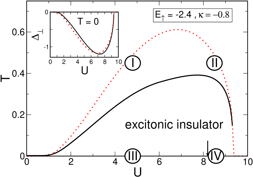
Figure 1: (Color online) Stability region of the EI phase in the 3D half-filled EFKM (the arrow marks the critical coupling where the Hartree gap (74) opens). The inset shows the order parameter at zero temperature. Red dotted curves give the Hartree-Fock results for comparison.

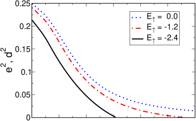
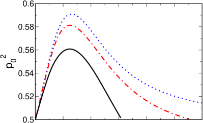
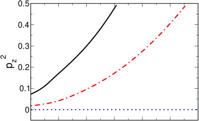
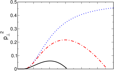
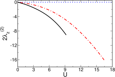
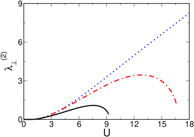
Figure 2: (Color online) $U$-dependence of slave-boson fields and Langrange parameters for different $E_{\uparrow}$ at $T=0$ ($\kappa=-0.8$).

The variation of the other bosonic fields is depicted in Fig. 2, where the solid curves belong to the parameter values used in Fig. 1. We see that the number of empty and double-occupied sites, $e^{2}$ and $d^{2}$, is equal and goes to zero at the EI-BI transition, where we have $p_{0}^{2}=p_{z}^{2}=1/2$ at singly occupied sites. Non-vanishing values of $p_{\perp}^{2}$ and $\lambda_{\perp}^{(2)}$ indicate an EI state, which demonstrates the importance of the (transverse) ‘spin-flip’ processes for the formation and maintenance of $f$-$c$ coherence. The slave-boson band shift $|2\lambda_{z}^{(2)}|$ in Eq. (II.3) increases with increasing $U$ (just as the Hartree shift). Obviously, the area of the EI phase is enlarged if one reduces the splitting of the $f$ and $c$ band centers (cf. the red dot-dashed lines). We include the data for the metastable EI solution at $E_{\uparrow}=0$ (as discussed above, in this case the charge-density-wave state will win), in order to show that $d^{2}$ and $e^{2}$ stay finite for all $U$. That means, for the orbital-degenerate EFKM ($\lambda_{z}^{(2)}=\tilde{\mu}=0$), our $SO(2)$-invariant slave-boson scheme will not give the (artificial) transition into an insulating Brinkmann-Rice-like correlated-insulator state Brinkman and Rice (1970). This transition is a well-known shortcoming of the scalar slave-boson approach to the Hubbard model Kotliar and Ruckenstein (1986) and has been also observed applying the scalar slave-boson theory to the EFKM Brydon (2008). The effect becomes even more apparent by comparing the variation of the slave-boson band-renormalization factors $z^{2}$.

Figure 3 shows that $z^{2}$ vanishes within the scalar slave-boson theory (right-hand panel) for $E_{\uparrow}=0$ at a critical interaction strength ($U_{\rm BR}\simeq 14.5$), indicating the localization of charge carriers, whereas in our theory the bandwidth will be only slightly renormalized at this point (see left-hand panel). Interestingly, the band renormalization is rather small in the EI phase as well (cf. the curves for $E_{\uparrow}=-1.2,\,-2.4$). Here we find $z^{2}\gtrsim 0.95$, which explains the small deviation of the slave-boson order parameter from its Hartree-Fock counterpart (see inset of Fig. 1).

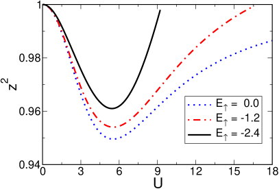
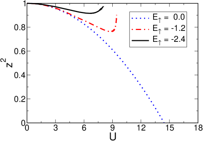
Figure 3: (Color online) Band-renormalization factors at $T=0$ within $SO(2)$-invariant (left-hand panel) and scalar (right-hand panel) slave-boson theory. Again, $\kappa=-0.8$.

Next we discuss the finite-temperature behavior. The variation of the EI order parameter and of the band-renormalization factor with $T$ at fixed $U$ is displayed in Fig. 4. Most important, in comparison with the Hartree-Fock data, the critical temperature for the EI-semimetal/semiconductor phase transition is significantly reduced (see also Fig. 1). Looking at $z^{2}(T)$, this may be attributed to the more precise treatment of correlations and occupation number fluctuations. At $T_{c}$, the order parameter vanishes, and we observe a cusp in $z^{2}$. Enhancing, above $T_{c}$, the temperature further, the band renormalization goes on, where $z^{2}$ now always decreases with increasing $U$.

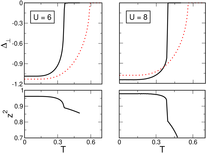
Figure 4: (Color online) $T$-dependence of the EI order parameter $\Delta_{\perp}$ and of the band renormalization $z^{2}$ at fixed Coulomb interaction $U=6$ (left-hand panels) and $U=8$ (right-hand panels). Red dotted lines show the corresponding Hartree-Fock data, where $z^{2}=1$. Band-structure parameters are the same as in Fig. 1.

Figure 5 shows the temperature dependencies of the various slave-boson fields and Lagrange parameters for $U=6$ (corresponding to the left-hand panel of Fig. 4). As expected, $p_{\perp}$ and $\lambda^{(2)}_{\perp}$ are monotonously decreasing functions of $T$, with $p_{\perp}(T_{c})=\lambda^{(2)}_{\perp}(T_{c})=0$. The other fields exhibit a cusp structure at $T_{c}$. At higher temperatures the probability of finding double occupied sites and empty sites increases. At the same time, we find less singly occupied sites ($\propto(p_{0}^{2}+p_{z}^{2})$), which means that the increase of $p_{0}^{2}$ is overcompensated by the reduction of $p_{z}^{2}$, indicating a more balanced occupation of $f$ and $c$ sites.

Figure 5: $T$-dependence of the various slave-boson fields for $U=6$, $E_{\uparrow}=-2.4$, and $\kappa=-0.8$.

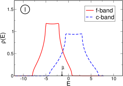
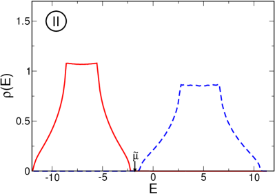
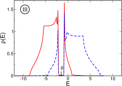
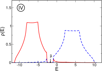
Figure 6: (Color online) Partial densities of states for $f$-band (red solid curves) and $c$-band (blue dashed curves) electrons at the points ($U=4.8,\,T=0.45$), (8.5, 0.45), (4.8, 0), (8.5, 0) marked by I-IV in Fig. 1. Band-structure parameters are $E_{\uparrow}=E_{f}=-2.4$ and $t_{\uparrow}=t_{f}=-0.8$.

Finally, we analyze the partial $f$ and $c$ electron density of states (DOS), $\rho_{\uparrow}(E)$ and $\rho_{\downarrow}(E)$, defined via

$$n_{\sigma}= \frac{1}{N}\sum_{\vec{k}}n_{\vec{k}\sigma}=\int dE\rho_{\sigma}(E)\,,$$ (81)

$$n_{\vec{k}\uparrow}= \tfrac{1}{2}(1+m_{\vec{k}})n_{\vec{k}+}+\tfrac{1}{2}(1-m_{\vec{k}})n_{\vec{k}-}\,,$$ (82)

$$n_{\vec{k}\downarrow}= \tfrac{1}{2}(1-m_{\vec{k}})n_{\vec{k}+}+\tfrac{1}{2}(1+m_{\vec{k}})n_{\vec{k}-}\,,$$ (83)

where $n_{(\vec{k})\sigma}$ are the corresponding particle densities. Figure 6 gives $\rho_{\uparrow,\downarrow}(E)$ at the characteristic $U$-$T$ points marked by I-IV in the phase diagram of Fig. 1. Obviously, the high-temperature phase may be viewed as a metal/semimetal (panel I) or a small-gap semiconductor (panel II) in the weak-to-intermediate or strong Coulomb-attraction regime. Accordingly, the EI phase at low temperatures shows different characteristics as well. As can be seen from panel III, a correlation-induced ‘hybridization’ gap opens in the DOS with $n_{-}=1$ ($n_{+}=0$) at $T=0$, indicating EI long-range order. The pronounced $c$–$f$ state mixing and strong enhancement of the DOS at the upper/lower valence/conducting band edges reminds a BCS-like pairing evolving from a (semi-) metallic state with a large Fermi surface above $T_{c}$. By contrast, the zero-temperature DOS shown in panel IV evolves from an already gapped high-temperature phase. Here, preformed pairs (excitons) may exist Bronold and Fehske (2006); Ihle et al. (2008), which undergo a BEC transition at $T_{c}$.

IV Summary

In this work we studied the extended Falicov-Kimball model with respect to the formation of an exciton condensate, which is related to the problem of electronic ferroelectricity. Motivated by the discrepancy concerning the existence of the excitonic insulator (EI) phase within the Hartree-Fock and scalar slave-boson approaches, we developed an $SO(2)$-invariant slave-boson theory. The main result is that our improved slave-boson scheme is capable of describing the EI phase in a parameter region agreeing, at zero temperature, with Hartree-Fock (and, in 2D, constrained path Monte Carlo) results. This is in striking contrast to recent findings by the scalar slave-boson approach Brydon (2008), which fails to detect the EI phase in the case of non-degenerate $f$ and $c$ orbitals. The agreement of the zero-temperature semimetal$\to$EI and EI$\to$band-insulator transition points with the Hartree-Fock and Monte Carlo values is ascribed to a rather weak band renormalization at $T=0$. At finite temperature, band-renormalization effects due to electronic correlations and particle number fluctuations become important, and, as a result, our slave-boson theory yields significantly lower transition temperatures than Hartree-Fock. From the analysis of the partial $f$, $c$, and quasiparticle densities of states, in the EI phase a crossover from a BCS-type condensate to a Bose-Einstein condensate of preformed excitons may be suggested. The results of our investigations may form the basis of forthcoming studies, e.g., on the effects of fluctuations around the saddle point, allowing the calculation of pseudo-spin and charge susceptibilities for the EFKM on an equal footing.

References

- Mott (1961) N. F. Mott, Philos. Mag. 6, 287 (1961).
- Knox (1963) R. Knox, in Solid State Physics, edited by F. Seitz and D. Turnbull (Academic Press, New York, 1963), p. Suppl. 5 p. 100.
- Halperin and Rice (1967) B. I. Halperin and T. M. Rice, in Solid State Physics, edited by F. Seitz, D. Turnbull, and H. Ehrenreich (Academic, New York, 1967), vol. 21, p. 115.
- Leggett (1980) A. J. Leggett, in Modern Trends in the Theory of Condensed Matter, edited by A. Pekalski and R. Przystawa (Springer-Verlag, Berlin, 1980).
- Comte and Nozières (1982) C. Comte and P. Nozières, J. Phys. (France) 43, 1069 (1982).
- Bronold and Fehske (2006) F. X. Bronold and H. Fehske, Phys. Rev. B 74, 165107 (2006).
- des Cloizeaux (1965) J. des Cloizeaux, J. Chem. Phys. Solids 26, 259 (1965).
- Kohn (1968) W. Kohn, in Many Body Physics, edited by C. de Witt and R. Balian (Gordon & Breach, New York, 1968).
- Keldysh and Kopaev (1965) L. V. Keldysh and H. Y. V. Kopaev, Sov. Phys. Sol. State 6, 2219 (1965).
- Kozlov and Maksimov (1965) A. N. Kozlov and L. A. Maksimov, Sov. Phys. JETP 21, 790 (1965).
- Jérome et al. (1967) D. Jérome, T. M. Rice, and W. Kohn, Physical Review 158, 462 (1967).
- Zittartz (1968) J. Zittartz, Physics Reports 165, 612 (1968).
- Nozières and Schmitt-Rink (1985) P. Nozières and S. Schmitt-Rink, J. Low Temp. Phys. 59, 195 (1985).
- Zimmermann and Stolz (1985) R. Zimmermann and H. Stolz, Phys. Status Solidi B 131, 151 (1985).
- Kremp et al. (2008) D. Kremp, D. Semkat, and K. Henneberger, Phys. Rev. B 78, 125315 (2008).
- Bronold et al. (2007) F. X. Bronold, G. Röpke, and H. Fehske, J. Phys. Soc. Japan, Suppl. A 76, 27 (2007).
- Bronold and Fehske (2008) F. X. Bronold and H. Fehske, Superlattices and Microstructures 43, 512 (2008).
- Bascones et al. (2002) E. Bascones, A. A. Burkov, and A. H. MacDonald, Phys. Rev. Lett. 89, 086401 (2002).
- Wakisaka et al. (2009) Y. Wakisaka, T. Sudayama, K. Takubo, T. Mizokawa, M. Arita, H. Namatame, M. Taniguchi, N. Katayama, M. Nohara, and H. Takagi, Phys. Rev. Lett. 103, 026402 (2009).
- Cercellier et al. (2007) H. Cercellier, C. Monney, F. Clerc, C. Battaglia, L. Despont, M. G. Garnier, H. Beck, and P. Aebi, L. Patthey, H. Berger, L. Forró, Phys. Rev. Lett. 99, 146403 (2007).
- Monney et al. (2009) C. Monney, H. Cercellier, F. Clerc, C. Battaglia, E. F. Schwier, C. Didiot, M. G. Garnier, H. Beck, and P. Aebi, H. Berger, L. Forró, L. Patthey, Phys. Rev. B 79, 045116 (2009).
- Neuenschwander and Wachter (1990) J. Neuenschwander and P. Wachter, Phys. Rev. B 41, 12693 (1990).
- Bucher et al. (1991) B. Bucher, P. Steiner, and P. Wachter, Phys. Rev. Lett. 67, 2717 (1991).
- Wachter et al. (2004) P. Wachter, B. Bucher, and J. Malar, Phys. Rev. B 69, 094502 (2004).
- Falicov and Kimball (1969) L. M. Falicov and J. C. Kimball, Phys. Rev. Lett. 22, 997 (1969).
- Ramirez et al. (1970) R. Ramirez, L. M. Falicov, and J. C. Kimball, Phys. Rev. B 2, 3383 (1970).
- (27) K. Kanda, K. Machida and T. Matsubara, Solid State Commun., 19, 651 (1976).
- Portengen et al. (1996a) T. Portengen, T. Östreich, and L. J. Sham, Phys. Rev. Lett. 76, 3384 (1996a).
- Batista (2002) C. D. Batista, Phys. Rev. Lett. 89, 166403 (2002).
- Batista et al. (2004) C. D. Batista, J. E. Gubernatis, J. Bonča, and H. Q. Lin, Phys. Rev. Lett. 92, 187601 (2004).
- Schneider and Czycholl (2008) C. Schneider and G. Czycholl, Eur. Phys. J. B 64, 43 (2008).
- Portengen et al. (1996b) T. Portengen, T. Östreich, and L. J. Sham, Phys. Rev. B 54, 17452 (1996b).
- Czycholl (1999) G. Czycholl, Phys. Rev. B 59, 2642 (1999).
- Farkašovský (1999) P. Farkašovský, Phys. Rev. B 59, 9707 (1999).
- Farkašovský (2008) P. Farkašovský, Phys. Rev. B 77, 155130 (2008).
- Ihle et al. (2008) D. Ihle, M. Pfafferott, E. Burovski, F. X. Bronold, and H. Fehske, Phys. Rev. B 78, 193103 (2008).
- Brydon (2008) P. M. R. Brydon, Phys. Rev. B 77, 045109 (2008).
- Li et al. (1989) T. Li, P. Wölfle, and P. J. Hirschfeld, Phys. Rev. B 40, 6817 (1989).
- Lechermann et al. (2007) F. Lechermann, A. Georges, G. Kotliar, and O. Parcollet, Phys. Rev. B 76, 155102 (2007).
- Kotliar and Ruckenstein (1986) G. Kotliar and A. E. Ruckenstein, Phys. Rev. Lett. 57, 1362 (1986).
- Frésard and Wölfle (1992) R. Frésard and P. Wölfle, J. Phys. Condens. Matter 4, 3625 (1992).
- Negele and Orland (1988) J. W. Negele and H. Orland, Quantum Many-Particle Systems (Addison–Wesley, Reading, MA, 1988).
- Hooijer and Van Himbergen (1987) G. Hooijer and Van Himbergen, Phys. Rev. B 36, 7678 (1987).
- Deeg and Fehske (1994) M. Deeg and H. Fehske, Phys. Rev. B 50, 17874 (1994).
- Deeg et al. (1994) M. Deeg, H. Fehske, and H. Büttner, Europhys. Lett. 26, 109 (1994).
- Fehske (1996) H. Fehske, Spin Dynamics, Charge Transport and Electron–Phonon Coupling Effects in Strongly Correlated Electron Systems, Habilitationsschrift, Universität Bayreuth (1996).
- Fehske et al. (1992) H. Fehske, M. Deeg, and H. Büttner, Phys. Rev. B 46, 3713 (1992).
- Trapper et al. (1994) U. Trapper, H. Fehske, M. Deeg, and H. Büttner, Z. Phys. B 93, 465 (1994).
- Brinkman and Rice (1970) W. F. Brinkman and T. M. Rice, Phys. Rev. B 2 (1970).