ALMA Memo 590
Atmospheric dispersion and the implications for phase calibration

Abstract

The success of any ALMA phase-calibration strategy, which incorporates phase transfer, depends on a good understanding of how the atmospheric path delay changes with frequency (e.g. Holdaway & Pardo 2001). We explore how the wet dispersive path delay varies for realistic atmospheric conditions at the ALMA site using the atm transmission code. We find the wet dispersive path delay becomes a significant fraction ($\gtrsim 5$ per cent) of the non-dispersive delay for the high-frequency ALMA bands ($\gtrsim 160$ GHz, Bands 5 to 10). Additionally, the variation in dispersive path delay across ALMA’s 4-GHz contiguous bandwidth is not significant except in Bands 9 and 10. The ratio of dispersive path delay to total column of water vapour does not vary significantly for typical amounts of water vapour, water vapour scale heights and ground pressures above Chajnantor. However, the temperature profile and particularly the ground-level temperature are more important. Given the likely constraints from ALMA’s ancillary calibration devices, the uncertainty on the dispersive-path scaling will be around 2 per cent in the worst case and should contribute about 1 per cent overall to the wet path fluctuations at the highest frequencies.

1 Introduction

The performance of interferometers at (sub)millimetre wavelengths is often limited by differential fluctuations in the atmospheric path along the line of sight to each of the constituent antennas. If uncorrected, these fluctuations lead to a loss in sensitivity, imaging artefacts and a limit on the maximum usable baseline (e.g. Carilli & Holdaway 1999; Asaki et al. 2005; Nikolic, Richer & Hills 2008). ALMA will correct such path variations using a combination of techniques:

1. Fast-switching observations of bright calibrator sources (e.g. quasars).

2. Water vapour radiometry using dedicated 183-GHz radiometers (WVRs), installed in every 12-m ALMA antenna. The WVRs will allow the retrieval of the amount of water vapour along the line of sight to each antenna and thus fluctuations in the atmospheric path length resulting from this water vapour.

3. Self calibration, for a fraction of the brightest science targets.

Fast switching interleaves science observations with short ($\sim$ a few seconds) calibration observations on a cycle time of 20–200 s. These calibrations allow an estimate of the atmospheric and instrumental phase errors in the direction of the calibrator. The applicability of the calibrator phase solutions to the science target depends on their angular separation and the observing frequency. The radiometric technique will be applied continuously, correcting for atmospheric path fluctuations on timescales shorter than the fast-switching cycle time, but does require an accurate model to convert the WVR measurements into path delays.

Variations in the atmospheric path delay to the antennas predominantly arise from a combination of fluctuations in the water vapour content and density of air in the troposphere – respectively, the so-called wet and dry path components. Furthermore, we can split both components (the wet and dry) into two parts: one dispersive (i.e. dependent on frequency) and the other non-dispersive (independent of frequency). Conventionally, the non-dispersive part is taken to be the path in the low-frequency limit. This memo focuses on the dispersive part of the wet path delay introduced by the atmosphere. Previously, atmospheric dispersion in the context of fast switching was studied by Holdaway & Pardo (2001) and Holdaway & D’Addario (2004). They found the magnitude of the dispersive phase will become non-negligible in ALMA’s submillimetre bands. Furthermore, Holdaway & Pardo (2001) quantified the dispersive phase delay for typical conditions at the ALMA site. We extend their work by investigating how the dispersive path delay depends on the variation of the physical parameters of the atmosphere and what constraints can be placed on it from the proposed ancillary calibration devices on site.

This memo is structured into six parts. First, we explain the planned phase-correction strategy for ALMA and where dispersive effects play a role. Second, in § 3, we describe how dispersive and non-dispersive path delays arise in the atmosphere and how we compute the dispersive path delay. § 3 also quantifies the dispersive path delay across the full range of ALMA observing frequencies, before § 4 demonstrates how varying different atmospheric parameters changes the magnitude of the dispersive path delay. Finally, we look at what constraints can be placed on the dispersive path delay with temperature measurements from weather-monitoring devices.

2 Phase calibration for ALMA

Before we consider the magnitude of the dispersive path delay, we will detail the current phase-correction plans for ALMA and how these are affected by atmospheric dispersion.

Numerous previous memos have discussed fast-switching phase correction for ALMA (e.g. Carilli & Holdaway 1999; Holdaway 2001; Holdaway & D’Addario 2004). Briefly, fast switching removes some of the antenna-based phase fluctuations by regularly making short observations of a bright point-source calibrator, close to the science target in the sky. This difference in direction between the target and calibrator means the calibration solutions need to be interpolated to estimate the science target’s phase errors.

Typically, at ALMA’s highest observing frequencies, it will be unlikely that the calibrations can be taken at the same frequency as the science observations, for the following reasons:

1. Calibrators of the necessary strength at the science frequency will probably be too far from the science target (although this depends on the source counts at high frequencies, which are currently not well known).

2. The combination of high frequencies and long baselines may resolve many potential calibrators.

3. The phase errors may prove to be so large that phase wrapping makes reliable solutions difficult.

To overcome these difficulties, one proposal is for ALMA to observe calibration sources at 90 GHz when necessary and then scale the corresponding phase solutions to the science frequency (the phase-transfer technique). The frequency above which the phase transfer-approach will be necessary depends on the array configuration, atmospheric conditions and ultimately experience gathered at the site. It is currently expected to be the routine mode at wavelengths below 2 mm (frequencies $\gtrsim 150$ GHz). In the absence of dispersion, the required phase scaling is simply the ratio of the calibration and science frequencies. However, at high frequencies, as we have already mentioned and will detail below, the numerous nearby water vapour lines ensure that atmospheric dispersion will need to be taken into account.

Fluctuations in the atmospheric path on timescales shorter than the fast-switching cycle time will be corrected radiometrically using WVRs installed in every 12-m ALMA antenna. The WVRs measure the brightness of the 183-GHz atmospheric water line, which is very sensitive to the total amount of water vapour in the atmosphere (Stirling et al., 2004; Nikolic, 2009a). The fundamental difficulty in the analysis of WVR data is how to convert fluctuations in the measured sky brightnesses around the 183-GHz water line into variations in the atmospheric path delay. We have begun to develop a Bayesian framework for computing such conversion factors (Nikolic, 2009a, b), which naturally incorporates the prior knowledge of the system and all the observable data. In the first memo (Nikolic, 2009a), we begin with the simplest possible model atmosphere, comprising a single, thin layer of water, which is the only cause of path fluctuations. Even so, an analysis of test data from prototype WVRs that were installed on the Submillimeter Array (SMA) yields corrections that are within $\sim 5$ per cent of optimal ones. Memo 588 (Nikolic, 2009b) extends this scheme to include the observed correlation between phase and sky brightness, which ALMA may implicitly record during fast switching, when the calibrator’s phase is measured whilst data are taken with the WVRs. The inclusion of this empirical relationship should significantly improve the accuracy of the phase correction.

Typically, the calculation of phase-correction coefficients (i.e. the conversion factors above) from WVR data requires a model of the atmosphere, which in principle can be used to estimate the dispersive as well as non-dispersive path delays. In our work to date, which was based on relatively low-frequency (220 GHz) data, we have not modelled the dispersive path contribution. Instead, we simply scale the non-dispersive path delay by a constant factor to estimate the total wet delay. However, in reality this factor is a function of frequency. Furthermore, if the dispersive contribution is a significant fraction of the total path delay, it must be determined with good accuracy. To date there has been little work on what atmospheric properties influence the magnitude of the dispersive path delay and by what amount. In § 4, we therefore examine the variation of the dispersive path delay using multiple realistic models of the atmosphere above the ALMA site.

3 The dispersive path delay

Fluctuations in the wet path delay, $\rmn{d}l_{\rmn}{H_{2}O}$, are separated into the sum of non-dispersive ($\rmn{d}s$) and dispersive delays ($\rmn{d}S_{\nu}$):

$$\rmn{d}l_{\rmn}{H_{2}O}=\rmn{d}s+\rmn{d}S_{\nu}.$$ (1)

The total non-dispersive path delay (i.e. the sum of the wet and dry components) can be computed from the Smith-Weintraub equation for the refractive index, $n$, at a temperature, $T$ (Stirling et al., 2008; Nikolic, 2009a):

$$n-1=10^{-6}\left[\alpha\frac{P_{\rmn}{d}}{T}+\beta\frac{P_{\rmn}{w}}{T}+\gamma\frac{P_{\rmn}{w}}{T^{2}}\right]\rmn{,}$$ (2)

where $P_{\rmn}{d}$ and $P_{\rmn}{w}$ are the partial pressures of the dry air and water vapour respectively and $\alpha$, $\beta$ and $\gamma$ are constants. Since we are only concerned with the excess path introduced by water vapour (i.e. d$s$ above), then we may omit the first term and of the remaining terms the last one dominates. Hence we can transform to the following expression (Nikolic, 2009a):

$$\rmn{d}s\approx\frac{1741\,\rmn{K}}{T}\rmn{d}c,$$ (3)

where $c$ is the water vapour column.

In general, atmospheres with spectral lines are dispersive, with the dispersion related to the absorption according to the Kramers-Krönig relations. Thus, any atmospheric property that affects the shapes of absorption-line features will probably influence the atmospheric dispersion, summarized in the following functional form (see Tab. 1 for a list of the symbols used):

$$\rmn{d}l_{\rmn}{H_{2}O}\approx\left(\frac{1741\,\rmn{K}}{T}\right)\rmn{d}c+\rmn{d}S_{\nu}(\nu,T,\Gamma,p,c),$$ (4)

where we have substituted the non-dispersive delay from Eq. 3 into Eq. 1. The variation of d$S_{\nu}$ as a function of its parameters is studied in the remainder of this memo.

3.1 Computing the dispersive path delay

We calculate the dispersive and non-dispersive contributions to the wet and dry path delays between 1 GHz and 1 THz from model atmospheres using the atm software (Pardo, Cernicharo & Serabyn, 2001). atm accurately predicts the atmospheric opacity above Mauna Kea, Hawai’i up to 1.6 THz (Pardo et al., 2005). Its dispersive calculations have not been as thoroughly verified due to a lack of high-frequency test data, which should change in the near future once the ALMA WVRs become operational at Chajnantor.

In Fig. 1, we plot the wet and dry, dispersive and non-dispersive path delays overlaid on top of the atmospheric transmission, all computed using the basic model parameters listed in Tab. 1, which are suitable for the ALMA array operations site (AOS) at Chajnantor. The parameters listed in Tab. 1 are the median values measured by site-monitoring equipment where possible and their origin will be detailed in later sections. The computed dispersive path delay is small except around the atmospheric H₂O lines (for the wet component) or O₂ lines (for the dry). The largest contribution to the total delay at all frequencies arises from the dry non-dispersive path delay. However, we expect the dry column to be relatively stable and so contribute very little to the differential path delay (Holdaway & Pardo, 2001; Holdaway & D’Addario, 2004) i.e. the difference in delay between antennas. We will ignore the dry path delays for the rest of this memo but they may prove to be a significant extra source of error that remain after phase correction using the WVRs.

Table 1: Basic parameters of the atmospheric model of the ALMA AOS site, computed from median site characterization data except $p_{\rmn}{g}$ (see Appendix  A for details).

Parameter	Units	Value	Comment
$c$	mm	1.22	Zenith water column
$p_{\rmn}{g}$	mb	560	Ground-level pressure
$T_{\rmn}{g}$	K	270	Ground-level temperature
$\Gamma_{\rmn}{T}$	K km-1	$-7.28$	Tropospheric lapse rate
$h_{0}$	km	1.16	Water vapour scale height

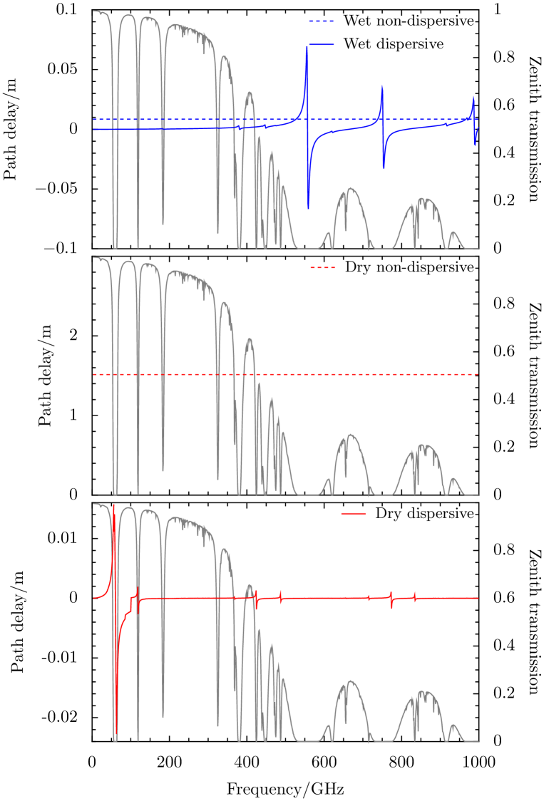
Figure 1: Wet non-dispersive (top panel, dashed blue) and dispersive (top panel, solid blue) path delays alongside the dry non-dispersive (middle panel, dashed red) and dispersive (bottom panel, solid red) path delays calculated by atm for the AOS model atmosphere with standard parameters as listed in Tab. 1, including a 1.22 mm column of water. Overlaid in grey on all three panels is the corresponding zenith atmospheric transmission, calculated from the total opacity, $\tau$ (as $e^{-\tau}$).

In Fig. 2, we plot the ratio of wet dispersive to non-dispersive path delay across the (currently-funded) ALMA observing bands (see Tab. 2). In the first two of these bands (Bands 3 and 4), the dispersive path delay is between 0.5 and 3 per cent of the non-dispersive, rising as a fraction approximately linearly with frequency. At the frequencies of Band 5 and higher, the dispersive path becomes a more significant fraction of the total wet delay ($\gtrsim 5$ per cent) and will need to be considered in both the fast-switching and WVR analyses. In Band 8 for instance, as far as possible from the absorption lines, the dispersive path delay is 20 to 40 per cent of the non-dispersive.

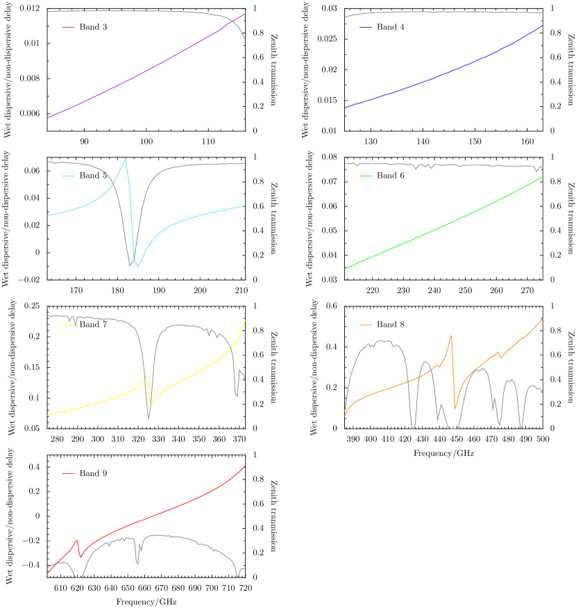
Figure 2: Ratio of the wet dispersive to wet non-dispersive delay for the construction ALMA observing bands, listed in Tab. 2. Also plotted (grey) is the atmospheric zenith transmission at the same frequency. The ratio rises continually with frequency and becomes particularly significant in the submillimetre bands (Bands 7, 8 & 9).

Table 2: ALMA receiver bands. In the initial phase of operations ALMA will be equipped with only six bands: 3,4, & 6–9. Bands 1 and 2 are not yet funded.

Band	Frequency	$T_{\rmn}{rx}$ 1	$\nu_{\mathrm{rep}}$ 2	Mixing 3	Supplier 4
	range (GHz)	(K)	(GHz)	Scheme
1	31–45	17	38	USB	–
2	67–90	30	79	LSB	–
3	84–116	37	100	2SB	HIA
4	125–163	51	144	2SB	NAOJ
5	163–211	65	200	2SB	OSO†
6	211–275	83	243	2SB	NRAO
7	275–373	147	342	2SB	IRAM
8	385–500	196	405	2SB	NAOJ
9	602–720	175	680	DSB	NOVA
10	787–950	230	869	DSB	NAOJ

¹ Receiver noise temperature specification for over 80 per cent of the band.
² Representative frequency, either the band centre or where the transmission is better if the centre is near an absorption line.
³ Two lowest-frequency bands use HEMT mixer technology and are single sideband, either upper (USB) or lower (LSB); all the others use SIS mixers and are either dual sideband (2SB – each sideband detected separately) or double sideband (DSB).
⁴ HIA – Herzberg Institute of Astrophysics, Canada; NAOJ – National Astronomical Observatory of Japan; OSO – Onsala Space Observatory/ Chalmers University, Sweden; NRAO – National Radio Astronomy Observatory, USA; IRAM - Institut de Radio Astronomie Millimétrique, France; NOVA – Nederlandse Onderzoekschool voor de Astronomie.
^† Six production receivers will be provided through the European Commission’s Framework 6 programme.

Additionally, we can investigate the phase slope that the atmosphere would introduce across the observing bandpass if no account were taken for variations in the dispersive path delay with frequency. In Fig. 3, we plot the fractional variation in the dispersive path delay for a 4-GHz portion of frequency space around representative band frequencies listed in Tab. 2. For each band we have normalized the values with respect to the chosen bandpass centre frequency. As we noted for Fig. 2, the dispersive path delay varies approximately linearly for small frequency widths. For most of the bands the variation is $\pm 2-5$ per cent over the observing bandwidth. Thus, such variation can be ignored, particularly at the lowest frequencies where the dispersive path delay makes a small contribution overall. Of the bands plotted, only Band 9 exhibits large variations of some $\pm 13$ per cent across the 4-GHz chunk, which rises to nearly $\pm 30$ per cent if the full 8-GHz DSB bandwidth is considered. In this case, a frequency-dependent scaling or multiple independent calculations of the dispersive phase (as planned in the ALMA correlator and TelCAL software sub-system) will be important.

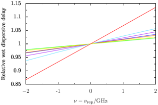
Figure 3: Variation in wet dispersive path delay for the construction ALMA bands, which were listed in Tab. 2. The lines use the same colours as Fig. 2 for the different bands: 3 (purple), 4 (dark blue), 5 (light blue), 6 (green), 7 (yellow), 8 (orange), 9 (red). The delays are plotted for frequencies in a 4-GHz portion around the bands’ representative frequencies (listed in Tab. 2, typically the band centres). This portion represents half of the instantaneous contiguous bandwidth (either the upper or lower sideband) for the ALMA 2SB mixers. Each measurement is divided by the value at the representative frequency and all the computations are for the median atmosphere specified in Tab. 1. The Band 9 receivers are DSB and therefore provide 8-GHz contiguous bandwidth (not plotted), which results in about a 30 per cent variation in the dispersive path delay towards the band edges compared with the representative frequency.

4 Physical influences on the dispersive path delay

In this section we quantify the impact of changes in atmospheric conditions on the wet dispersive path delay. We explore the influence of: the quantity of water vapour (§ 4.1), the ground-level temperature (§ 4.2) and pressure (§ 4.3) alongside the distribution of temperature with height (§ 4.4) and the distribution of water vapour with height (§ 4.5). For each investigation we compute the dispersive delay from atm using a variety of atmospheric models designed to represent average and extreme conditions at the ALMA AOS.

Our focus is the radiometric phase-correction technique using the WVRs. An important requirement for this technique is the optimal computation of time-dependent phase-correction coefficients, d$L/$d$T_{\rmn{B},i}$, for each of the four WVR channels. These coefficients relate a change in atmospheric path, $\delta L$, to a change in the observed sky brightness by a WVR, in each of its four channels, $\delta T_{\rmn{B},i}$, via (see Nikolic 2009a, b):

$$\delta L=\sum_{i=1}^{4}w_{i}\frac{\rmn{d}L}{\rmn{d}T_{\rmn{B},i}}\delta T_{\rmn{B},i}\rmn{,}$$ (5)

where $w_{i}$ is an appropriate weighting for each channel. We can decompose this expression further, since the WVRs are really only sensitive to variations in the water vapour column, $\delta c$, which we can relate to the measured sky brightness by introducing coefficients, d$c/$d$T_{\rmn{B},i}$:

$$\delta c=\sum_{i=1}^{4}w_{i}\frac{\rmn{d}c}{\rmn{d}T_{\rmn{B},i}}\delta T_{\rmn{B},i}\rmn{.}$$ (6)

Although the WVRs do place constraints on the atmospheric temperature and pressure, normally they cannot detect small fluctuations in their values. We can then write the variation in wet path delay, $\delta l_{\rmn}{H_{2}O}$, as the product of the fluctuation in water vapour content and the sum of two scaling terms:

$$\delta l_{\rmn}{H_{2}O}=\left(\frac{1741\,\rmn{K}}{T}+\frac{\rmn{d}S_{\nu}}{\rmn{d}c}\right)\delta c.$$ (7)

The first scaling term is the non-dispersive path delay from Eq. 3, while the second quantifies the dispersive path delay. Finally, as we saw in § 3, although d$S_{\nu}$/d$c$ may vary a lot, it is only related to the dispersive path delay, which in the millimetre bands makes a very small contribution to the total path delay compared to the non-dispersive path.

4.1 Water vapour quantity

First, we investigate the effect of varying the column of water vapour, $c$, in the standard AOS atmosphere (Tab. 1). In Fig. 4 we plot $\Delta S_{\nu}/\Delta c$ for $c=0.44$, 0.69, 1.22, 2.56 and 5.45 mm corresponding to the 10, 25, 50, 75 and 90 percentiles of the precipitable water vapour (PWV) cumulative function at Chajnantor respectively. These percentiles are derived from the cumulative 225 GHz opacity distributions as described in § A.1 of Appendix  A. Fig. 4 is the template for all the plots that follow in this section. The upper panels display the absolute variation in $\Delta S_{\nu}/\Delta c$ for the full extent of the ordinate (left panel) and for an enlarged portion close to the horizontal axis (right panel). In the lower panels, we plot the relative change in $\Delta S_{\nu}/\Delta c$, computed by dividing its spectrum (i.e. $\Delta S_{\nu}/\Delta c$ as a function of frequency) by the one from the median column, $c=1.22$ mm. Again, on the left-hand side we show the full ordinate range, whilst on the right we enlarge the plot around a ratio of unity.

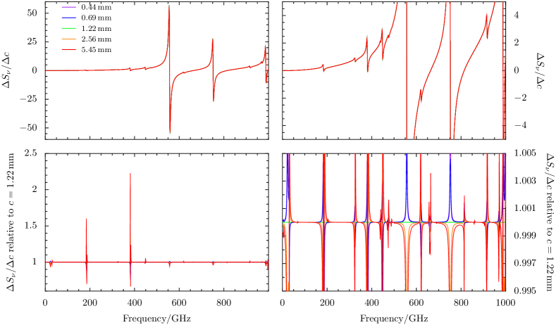
Figure 4: Variation of $\Delta S_{\nu}/\Delta c$ with column of water, $c$. The upper panels show the absolute variation in $\Delta S_{\nu}/\Delta c$ as a function of frequency from 1 to 1000 GHz, while the lower panels show the variation relative to (i.e. divided by) the median profile with $c=1.22$ mm. The right-hand panels show the same data as in left-hand ones but over a narrower range of values. The plotted data come from profiles containing 0.44, 0.69, 1.22, 2.56 and 5.45 mm of water respectively corresponding to the 10, 25, 50, 75 and 90 percentiles of the PWV cumulative function at Chajnantor (see § A.1). All the curves are plotted in each of the panels: if only one line is discernible then the curves overlap.

The shape of the $\Delta S_{\nu}/\Delta c$ spectrum closely resembles that of the dispersive path delay overall, i.e. $\Delta S_{\nu}$ is proportional to $\Delta c$ (see Fig. 1), having discontinuities where the dispersive path delay wraps around, near the dips of the atmospheric transmission and bright water lines. Even in the enlarged (upper right panel) and relative plots (lower panels) there are no discernible differences between $\Delta S_{\nu}/\Delta c$ for the different values of $c$. The only significant departures from unity for the relative $\Delta S_{\nu}/\Delta c$ are at discontinuities in $\Delta S_{\nu}/\Delta c$. Correspondingly, over the entire range of conditions likely at the ALMA AOS, the amount of water vapour does not affect $\Delta S_{\nu}/\Delta c$, only supplying a non-dispersive linear change. Furthermore, varying the telescope’s elevation/line of sight airmass has an equivalent effect to altering the water vapour column at zenith. Therefore our plots also indicate that the dispersive phase scaling does not depend on airmass and will not need to be recomputed for changes in elevation during observing.

4.2 Air temperature at ground level

Next, we look at how the ground-level temperature affects the predicted phase-correction coefficients. As in the previous section (§ 4.1), we varied $T_{\rmn}{g}$, in the standard AOS atmosphere which was used as the input to atm. Fig. 5 provides our results for $\Delta S_{\nu}/\Delta c$, in the same format as Fig. 4, using $T_{\rmn}{g}=262$, 265, 270, 276 and 281 K corresponding to the 10, 25, 50, 75 and 90 percentiles of the temperature cumulative function at Chajnantor (Radford, 2004).

The key plot is in the lower right panel, where we plot the spectrum for each $T_{\rmn}{g}$ relative to 270 K. The relative $\Delta S_{\nu}/\Delta c$ computed are constant with frequency except at the centres of absorption features, i.e. the same frequencies as in Fig. 4. The variation in the ratio at different $T_{\rmn}{g}$ is higher than for the different water vapour columns, and therefore will have more significance. Between the 25 and 75 percentiles, the difference in $\Delta S_{\nu}/\Delta c$ is 5–6 per cent but at the 10 and 90 percentiles it becomes 7–9 per cent. These differences are likely to be non-negligible for phase correction at submillimetre frequencies.

This variation is also important if we recall the strong diurnal change in temperature at Chajnantor. Stirling et al. (2006) found the temperature varied between approximately $-5$ and $5^{\circ}$C at their site A over 24 hours. Such a change could alter the dispersive path delay scaling by around $\pm 5$ per cent. We return to the constraints we can place on this source of uncertainty using meteorological data from the ALMA ancillary calibration devices in § 5.

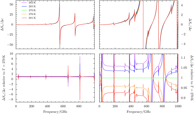
Figure 5: Variation of $\Delta L/\Delta c$ with ground temperature, $T_{\rmn}{g}$. Panels are laid out as for Fig. 4. The plotted data have $T_{\rmn}{g}$ of 262, 265, 270, 276, 281 K corresponding to the 10, 25, 50, 75 and 90 percentiles of the temperature cumulative function at Chajnantor. The temperature data are from Radford (2004).

4.3 Air pressure at ground level

We have checked the impact of changing the air pressure at ground level, $p_{\rmn}{g}$, by repeating the previous atm calculations using our standard AOS atmosphere with $p_{\rmn}{g}$ set to 520, 540, 560, 580, 600 mb. The results, shown in Fig. 6, indicate that $\Delta S_{\nu}/\Delta c$ varies $p_{\rmn}{g}$ at a level typically less than 0.2 per cent. This is much smaller than the effect resulting from any of the other atmospheric parameters we consider, so $p_{\rmn}{g}$ is not a likely source of uncertainty in the WVR phase-correction coefficients.

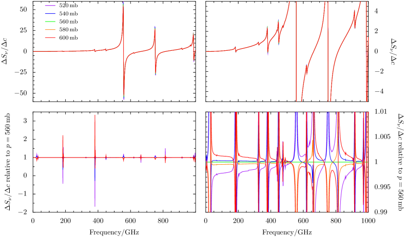
Figure 6: Variation of $\Delta L/\Delta c$ with ground pressure, $p_{\rmn}{g}$. Panels are laid out as for Fig. 4. The plotted data have $p_{\rmn}{g}$ of 520, 540, 560, 580, 600 mb.

4.4 Tropospheric lapse rate

The main way in which we parameterize the vertical temperature distribution of the model atmospheres is through the tropospheric lapse rate, $\Gamma_{\rmn}{T}$. We investigate the effect of variations in $\Gamma_{\rmn}{T}$ on the dispersive path delay in Fig. 7, where $\Delta S_{\nu}/\Delta c$ is plotted for $\Gamma_{\rmn}{T}=-4.80,-5.69,-7.28,-8.83,-9.71$ K km^-1. These $\Gamma_{\rmn}{T}$ again correspond to the 10, 25, 50, 75 and 90 percentiles of the $\Gamma_{\rmn}{T}$ distribution, which we derive from radiosonde data as explained in § A.2. Realistic variations in the lapse rate at the AOS will produce small, non-negligible changes in the dispersive path scaling of some 2–3 per cent from median values. Later in § 5, we look at how well we can constrain the lapse rate and thus the path scaling using the proposed atmospheric temperature profiler for ALMA.

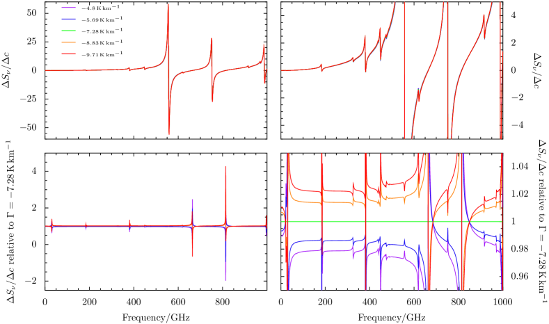
Figure 7: Variation of $\Delta L/\Delta c$ with tropospheric lapse rate, $\Gamma_{\rmn}{T}$. Panels are laid out as for Fig. 4. The plotted data have $\Gamma_{\rmn}{T}$ of $-4.80$, $-5.69$, $-7.28$, $-8.83$, $-9.71$ K km^-1 corresponding to the 10, 25, 50, 75 and 90 percentiles of the $\Gamma_{\rmn}{T}$ cumulative function at Chajnantor (see § A.2). $-10.0$ K km^-1 is the dry adiabatic lapse rate found in very dry atmospheres.

4.5 Scale height of atmospheric water vapour

The final parameter we interogate is the water vapour scale height, $h_{0}$. $\Delta S_{\nu}/\Delta c$ is plotted in Fig. 8 for $h_{0}=0.97$, 1.06, 1.16, 1.29, 1.54 km corresponding to the 10, 25, 50, 75 and 90 percentiles of the water vapour scale height cumulative function at Chajnantor (see § A.2). The relative dependence of $\Delta S_{\nu}/\Delta c$ on $h_{0}$ is again similar to the other parameters, i.e. it has spikes at the centres of absorption features. The relative $\Delta S_{\nu}/\Delta c$ typically varies from the median spectrum by between 0.5 and 1 per cent, which rises to 2–4 per cent in the 10 and 90 percentile cases. Thus, under the typical range of conditions at the site, $h_{0}$ is a small source of uncertainty in the dispersive scaling for phase correction.

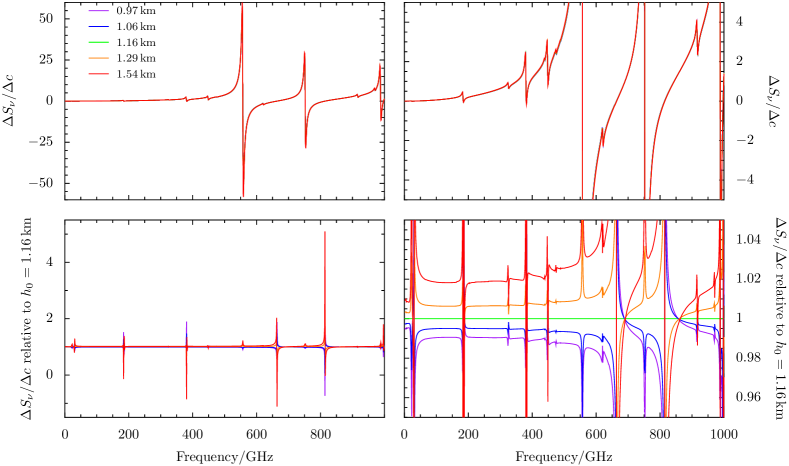
Figure 8: Variation of $\Delta L/\Delta c$ with water vapour scale height, $h_{\rmn}{0}$. Panels are laid out as for Fig. 4. The plotted data have $h_{0}$ of 0.97, 1.06, 1.16, 1.29, 1.54 km corresponding to the 10, 25, 50, 75 and 90 percentiles of the water vapour scale height cumulative function at Chajnantor.

5 Constraints from the ancillary calibration devices

Our predictions from the atmospheric models above indicate that the natural variation of certain atmospheric properties at the ALMA site could introduce non-negligible errors in the estimation of phase-correction coefficients and also in the phase-transfer scaling. However, ALMA will be equipped with a suite of ancillary calibration devices, including five meteorological towers and a temperature profiler, which will monitor basic atmospheric parameters such as the pressure, temperature and wind speed. In this section, we look at what constraints the temperature devices should be able to place on the dispersive path delay prediction.

First, we examine the ground temperature measurement. Although temperature probes will be positioned on every meteorological tower and possibly on some of the antennas, we are unlikely to be able to measure $T_{\rmn}{g}$ very accurately for each antenna. This is mainly because the temperature profile for the first 100 m of the atmosphere above the ALMA site is strongly controlled by surface heating and cooling, which results in variations of $\pm 5$ K over the site (Stirling et al., 2006). Therefore, we estimate we will be able to measure $T_{\rmn}{g}$ to around $\pm 2$ K for each antenna.

Using the standard AOS atmosphere with $T_{\rmn}{g}=270$ K as the input to atm, we computed the relative change in $\Delta S_{\nu}/\Delta c$ for a 1 and 2 K change in $T_{\rmn}{g}$, which we plot in Fig. 9. At frequencies where the dispersive phase makes a significant contribution to the overall path delay ($\gtrsim 345$ GHz), an estimate of the ground temperature to $\pm 2$ K can constrain the dispersive phase-correction coefficient to $\pm 1.5-2.0$ per cent. This is just under the limit of what would be acceptable in a total phase calibration budget of 2 per cent. If we could do better and constrain $T_{\rmn}{g}$ to $\pm 1$ K, then we could get to better than a 1 per cent error.

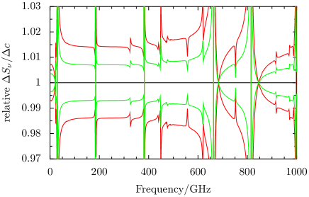
Figure 9: Constraints placed on the dispersive $\Delta S_{\nu}/\Delta c$ from a measurement of $T_{\rmn}{g}$. The lines plot the relative change in $\Delta S_{\nu}/\Delta c$ from the median $T_{\rmn}{g}$ (270 K) spectrum, when $T_{\rmn}{g}$ is changed by 1 K (green) or 2 K (red).

ALMA also plans to utilize an atmospheric temperature profiler, which will use multi-frequency observations of the sky brightness around the 60 GHz O₂ lines to infer the atmospheric temperature profile. Such a profile will provide information about the air temperature away from the ground where surface effects are minimized and the values are probably more settled. The current specifications of the profiler unit state it will measure the atmospheric temperature to $\Delta T\leq 2$ K with a vertical resolution of $\Delta z\leq 200$ m up to 1500 m above the AOS. We assume the temperature profile consists of 8 measurements of the temperature separated vertically by 200 m, and each accurate to $\pm 2$ K. If the profile is a straight line, we can perform a least-squares fit, which should measure the lapse rate, $\Gamma$, to $\pm 1.5$ K km^-1. If the accuracy of each temperature measurement is better, say to $\pm 1$ K, then the corresponding accuracy on $\Gamma$ reduces to $\pm 0.8$ K. Taking these constraints on the lapse rate in the standard AOS atmosphere, i.e. $\Gamma_{\rmn}{T}=-7.28\pm 1.5$ K km^-1, we plot the relative change in $\Delta S_{\nu}/\Delta c$ in Fig. 10. The plot looks very similar to Fig. 9. The error on $\Delta S_{\nu}/\Delta c$ in the submillimetre windows, where the dispersion is significant, is between 1 and 2 per cent using the information from the temperature profiler. If the accuracy of the profiler exceeds specifications to measure the temperature to $\pm 1$ K then this constraint reduces to around 0.5–1 per cent.

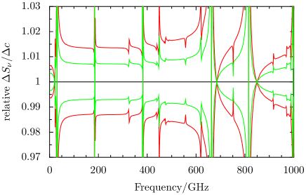
Figure 10: Constraints placed on the dispersive $\Delta S_{\nu}/\Delta c$ from a measurement of lapse rate by the atmospheric temperature profiler. The lines show the relative change in $\Delta S_{\nu}/\Delta c$ from the typical $\Gamma_{\rmn}{T}=-7.28$ K km^-1 spectrum, when $\Gamma_{\rmn}{T}$ is changed by 0.8 K km^-1 (green) or 1.5 K km^-1 (red).

6 Summary

Both of the primary phase-calibration techniques for ALMA rely on accurate estimates of how the atmospheric path fluctuations vary with frequency, because:

1. The phase solutions need to be scaled from the calibration to the science frequency for phase-transfer fast-switching.

2. The WVRs essentially measure variations in the quantity of water vapour, which must be converted into fluctuations in the phase delay of the incoming signal.

First, we revisited the magnitude of the wet dispersive path delay in a median AOS atmosphere using the atm software:

• In Bands 3 and 4 (84–163 GHz), the wet dispersive path delay is a small fraction, 0.5–3 per cent, of the wet non-dispersive path delay.

• For Bands 5 and above (163–720 GHz), the wet dispersive path delay becomes a significant fraction of the non-dispersive, $\gtrsim 5$ per cent and should be considered in any analysis, particularly at the highest frequencies. In the worst case, Band 8 (385–500 GHz), the dispersive path delay is 20–55 per cent of the non-dispersive.

• The variation in the dispersive path delay across the 4-GHz instantaneous bandwidth of a single observation is typically 2–5 per cent but does rise to higher fractions, $\sim$13 per cent, in Band 9. Thus, the capability of the ALMA correlator and software to apply phase corrections channel-by-channel will prove useful.

Next, we investigated how the the dispersive path delay changes when the model parameters were varied, over ranges that represented the typical and extreme atmospheric conditions measured above the ALMA site:

• The amount of atmospheric water vapour or equivalently the airmass does not affect $\Delta S_{\nu}/\Delta c$, i.e. the dispersive path contribution to the fluctuations.

• The typical changes in the water vapour scale height and ground pressure do produce small changes ($\lesssim 2$ per cent) to $\Delta S_{\nu}/\Delta c$.

• The dispersive path delay depends more strongly on the temperature profile of the atmosphere, particularly the air temperature at the ground. The 10 to 90 percentiles of the Chajnantor ground-temperature distribution cause variations in the dispersive $\Delta S_{\nu}/\Delta c$ of 7–9 per cent from the median. Additionally, typical diurnal variations in temperature ($\pm 5$ K) would produce similar changes of $\pm 5$ per cent. This will be significant at frequencies where the dispersive path delay provides a major contribution to the total path delay ($\gtrsim 345$ GHz). $\Delta S_{\nu}/\Delta c$ also depends on $\Gamma_{\rmn}{T}$ with the typical variation being some 2–3 per cent.

These results indicate that obtaining a ground-level air temperature estimate for each antenna to an accuracy of about $\pm 2$ K will reduce uncertainties in the models of the dispersive phase to a satisfactory level. In combination with lapse rate estimates, our calculations suggest that the ancillary calibration instruments on site should be able to constrain the dispersive terms to 1–2 per cent, on target for the current calibration budget.

The relatively small expected variation of dispersive path scaling with the natural range of atmospheric conditions at the AOS is also encouraging from the perspective of empirical models, which use the observed correlations between phase and WVR measurements. Because the variation is small, it means that the frequency-dependence of such empirical models will not need to be re-calibrated very often.

Appendix A Distributions of site-characterization parameters

A.1 Water vapour column

The quantity of water vapour above Chajnantor is not a directly-observable quantity. Instead, we calculate it from the measured atmospheric opacity using an appropriate scaling for the site. NRAO has operated an automated tipping radiometer at 225 GHz on the Chajnantor plateau since 1995 and the data up to August 2004 are collected online (Radford, 2004). We summarize the various cumulative distributions for $\tau_{225}$ used in the ALMA memo series and online in Tab. 3.

Table 3: Percentiles of the cumulative $\tau_{225}$ distribution above Chajnantor presented in previous work.

Percentile	$\tau_{225}$ 1	$\tau_{225}$ 2	$\tau_{225}$ 3	$\tau_{225}$ 4
25	0.036	0.037	0.037	0.037
50	0.061	0.061	0.062	0.060
75	0.115	0.122	0.125	0.118

¹ Memo 334 (Radford & Chamberlin, 2000), spanning 04/95 – 07/00.
² Memo 471 (Evans et al., 2003), spanning 04/95 – 08/01.
³ Memo 512 (Otárola et al., 2005), spanning 04/95 – 08/03.
⁴ The latest publicly-available data (Radford, 2004), spanning 04/95 – 12/04.

Various memos have also computed the conversion relation between $\tau_{225}$ and the PWV column (e.g. Delgado et al. 1999; Bustos et al. 2000). We use the relation presented in Giovanelli et al. (2001):

$$\tau_{225}=0.0435(\rmn{PWV}/\rmn{mm})+0.0068\rmn{,}$$ (8)

which is derived for Chajnantor from a comparison of $\tau_{225}$ to the PWV derived from a 183-GHz WVR and agrees well with radiosonde data for PWV¡3 mm. Using the standard atmospheric parameters we presented in Tab. 1, we also calculated the following conversion from atm:

$$\tau_{225}=0.0416(\rmn{PWV}/\rmn{mm})+0.0120\rmn{.}$$ (9)

This is similar to Eq. 8 but we prefer the experimentally-derived scaling as it has been tested more thoroughly. In Tab. 4 we list the percentiles of the PWV distribution which we use in this memo, derived from the most recent cumulative $\tau_{225}$ distribution that is publicly available (Radford, 2004) using Eq. 8.

Table 4: Percentiles of the cumulative $\tau_{225}$ and $c$ distributions above Chajnantor used in this memo. $c$ has been calculated from $\tau_{225}$ using Eq. 8.

Percentile	$\tau_{225}$ 1	$c$ (mm)
10	0.026	0.44
25	0.037	0.69
50	0.060	1.22
75	0.118	2.56
90	0.244	5.45

¹ Latest publicly-available site characterization data (Radford, 2004), spanning 04/95 – 12/04.

A.2 Parameters of the atmospheric vertical profile

To derive distributions of atmospheric parameters which depend on the variation of water vapour pressure and temperature with height through the atmosphere, we make use of the library of radiosonde launch data above the Chajnantor plateau. These radiosonde flights were jointly operated by Cornell University, NRAO, ESO and the Smithsonian Astrophysical Observatory between October 1998 and December 2001. The data and an analysis of each dataset are available on dedicated web pages. A preliminary analysis of these data was presented in Giovanelli et al. (2001). They show the vertical distribution of water vapour density in a median atmosphere derived from 108 launches is well approximated by an exponential with scale height $h_{0}=1.135$ km. We present the cumulative distribution of $h_{0}$ in Tab. 5. This is constructed using the analyses of Bryan Butler, which fitted an exponential to the water vapour pressure between 0 and 10 km above the Chajnantor plateau for each radiosonde launch. We include 194 separate launches over varying months and times of day.

Table 5: Percentiles of the cumulative $h_{0}$ distribution used in this memo, constructed by Bryan Butler who fitted an exponential function to the data between 0 and 10 km above Chajnantor (see http://www.tuc.nrao.edu/alma/site/Chajnantor/instruments/radiosonde).

Percentile	$h_{0}$ (km)
10	0.97
25	1.06
50	1.16
75	1.29
90	1.54

Furthermore, to ascertain the distribution of the tropospheric lapse rate, $\Gamma_{\rmn}{T}$ (Tab. 6), we fit a straight line to the radiosonde temperature data from 204 launches using a least-squares method. As most of the water vapour is concentrated in the first layers of the atmosphere we fit only to data in the first 1 km above the plateau surface. We note that in reality few temperature profiles from radiosonde data are a perfect straight line and some show more complicated features such as temperature inversions. However, for the purposes of this memo a simple fit should be sufficient.

Table 6: Percentiles of the cumulative $\Gamma_{\rmn}{T}$ distribution above Chajnantor used in this memo. It is constructed from fits to the temperature data $\leq 1$ km from the Earth’s surface at Chajnantor (see http://www.tuc.nrao.edu/alma/site/Chajnantor/instruments/radiosonde).

Percentile	$\Gamma_{\rmn}{T}$ (K km-1)
10	$-9.71$
25	$-8.83$
50	$-7.28$
75	$-5.69$
90	$-4.80$

References

- Asaki et al. (2005) Asaki Y., Saito M., Kawabe R., Koh-ichiro Morita K.-i., Tamura Y., Vila-Vilaro B., 2005, Simulation Series of a Phase Calibration Scheme with Water Vapor Radiometers for the Atacama Compact Array, ALMA Memo 515, The ALMA Project
- Bustos et al. (2000) Bustos R., Delgado G., Nyman L.-A., Radford S., 2000, 53 years of Climatological Data for the Chajnantor Area, ALMA Memo 333, The ALMA Project
- Carilli & Holdaway (1999) Carilli C. L., Holdaway M. A., 1999, Tropospheric Phase Calibration in Millimeter Interferometry, ALMA Memo 262, The ALMA Project
- Delgado et al. (1999) Delgado G., Otárola A., Belitsky V., Urbain D., Hills R., Martin-Cocher P., 1999, The Determination of Precipitable Water Vapour at Llano de Chajnantor from Observations fo the 183 GHz Water Line, ALMA Memo 271.1, The ALMA Project
- Evans et al. (2003) Evans N., Richer J., Sakamoto S., Wilson C., Mardones D., Radford S., Cull S., Lucas R., 2003, Site Properties and Stringency, ALMA Memo 471, The ALMA Project
- Giovanelli et al. (2001) Giovanelli R., Darling J., Henderson C., Hoffman W., Barry D., Cordes J., Eikenberry S., Gull G., Keller L., Smith J. D., Stacey G., 2001, PASP, 113, 803
- Holdaway (2001) Holdaway M. A., 2001, Fast Switching Phase Correction Revisited for 64 12 m Antennas, ALMA Memo 403, The ALMA Project
- Holdaway & D’Addario (2004) Holdaway M. A., D’Addario L., 2004, Simulation of Atmospheric Phase Correction Combined With Instrumental Phase Calibration Using Fast Switching, ALMA Memo 523, The ALMA Project
- Holdaway & Pardo (2001) Holdaway M. A., Pardo J. R., 2001, Atmospheric Dispersion and Fast Switching Phase Calibration, ALMA Memo 404, The ALMA Project
- Nikolic (2009a) Nikolic B., 2009a, Inference of Coefficients for Use in Phase Correction I, ALMA Memo 587, The ALMA Project
- Nikolic (2009b) Nikolic B., 2009b, Inference of Coefficients for Use in Phase Correction II: Using the Observed Correlation between Phase and Sky Brightness, ALMA Memo 588, The ALMA Project
- Nikolic et al. (2008) Nikolic B., Richer J. S., Hills R. E., 2008, Simulating Atmospheric Phase Errors, Phase Correction and the Impact on ALMA Science, ALMA Memo 582, The ALMA Project
- Otárola et al. (2005) Otárola A., Holdaway M., Nyman L.-A., Radford S. J. E., Butler B. J., 2005, Atmospheric Transparency at Chajnantor: 1973–2003, ALMA Memo 512, The ALMA Project
- Pardo et al. (2001) Pardo J. R., Cernicharo J., Serabyn E., 2001, IEEE Trans. on Antennas and Propagation, 49, 1683
- Pardo et al. (2005) Pardo J. R., Serabyn E., Wiedner M. C., Cernicharo J., 2005, J. Quant. Spectrosc. and Radiative Transfer, 96, 537
- Radford (2004) Radford S., 2004, Chajnantor Site Characterization Data, 1995-2004, http://www.tuc.nrao.edu/alma/site/Chajnantor/data.c.html
- Radford & Chamberlin (2000) Radford S. J. E., Chamberlin R. A., 2000, Atmospheric Transparency at 225 GHz over Chajnantor, Mauna Kea, and the South Pole, ALMA Memo 334.1, The ALMA Project
- Stirling et al. (2004) Stirling A., Hills R., Richer J., Pardo J., 2004, 183 GHz water vapour radiometers for ALMA: Estimation of phase errors under varying atmospheric conditions., ALMA Memo 496, The ALMA Project
- Stirling et al. (2006) Stirling A., Otárola A., Rivera R., Ruben Bravo J., 2006, Horizontal Temperature Variations at Chajnantor, ALMA Memo 541, The ALMA Project
- Stirling et al. (2008) Stirling A., Richer J., Hills R., Lock A., 2008, Turbulence simulations of dry and wet phase fluctuations at Chajnantor. Part I: The daytime convective boundary layer., ALMA Memo 517.1, The ALMA Project