Noise driven dynamic phase transition in a one-dimensional Ising-like model

Abstract

The dynamical evolution of a recently introduced one dimensional model in biswas-sen (henceforth referred to as model I), has been made stochastic by introducing a parameter $\beta$ such that $\beta=0$ corresponds to the Ising model and $\beta\to\infty$ to the original model I. The equilibrium behaviour for any value of $\beta$ is identical: a homogeneous state. We argue, from the behaviour of the dynamical exponent $z$, that for any $\beta\neq 0$, the system belongs to the dynamical class of model I indicating a dynamic phase transition at $\beta=0$. On the other hand, the persistence probabilities in a system of $L$ spins saturate at a value $P_{sat}(\beta,L)=(\beta/L)^{\alpha}f(\beta)$, where $\alpha$ remains constant for all $\beta\neq 0$ supporting the existence of the dynamic phase transition at $\beta=0$. The scaling function $f(\beta)$ shows a crossover behaviour with $f(\beta)=\rm{constant}$ for $\beta<<1$ and $f(\beta)\propto\beta^{-\alpha}$ for $\beta>>1$.

The effect of noise on equilibrium behavior is well known, e.g., there are order-disorder phase transitions induced by thermal noise observed in many systems. Noise induced phase transitions may occur in dynamical systems as well when the noise can drive the system from one dynamical class to another. These dynamical classes are often characterised by different dynamical exponents. In this paper, we study a case of such a dynamical phase transition in a very simple Ising like spin system.

A dynamical model of Ising spins has been recently proposed in biswas-sen (which we refer to as model I henceforth) where the state of the spins may change in two situations: first when its two neighbouring domains have opposite polarity, and in this case the spin orients itself along the spins of the neighbouring domain with the larger size. This case may arise only when the spin is at the boundary of the two domains. A spin is also flipped when it is sandwiched between two domains of spins with same sign. Except for the rare event when the two neighbouring domains of opposite spins are of the same size, the dynamics in the above model is deterministic. This dynamics leads to a homogeneous state of either all spin up or all spin down. Such evolution to absorbing homogeneous states are known to occur in systems belonging to directed percolation (DP) processes, zero temperature Ising model, voter model etc absorb ; vote .

Model I was introduced in the context of a social system where the binary opinions of individuals are represented by up and down spin states. In opinion dynamics models, such representation of opinions by Ising or Potts spins is quite common opinion1 . The key feature is the interaction of the individuals which may lead to phase transitions between a homogeneous state to a heterogeneous state in many cases opinion2 .

Model I showed the existence of novel dynamical behaviour in a coersening process when compared to the dynamical behaviour of DP processes, voter model, Ising models etc hinrich2 ; stauffer2 ; sanchez ; shukla ; derrida . In this work, we have introduced stochasticity in the dynamics of Model I to see how it affects the coarsening process.

Let $d_{up}$ and $d_{down}$ be the sizes of the two neighbouring domains of type up and down of a spin at the domain boundary (excluding itself). In model I, probability $P(up)$ that the said spin is up is 1 if $d_{up}>d_{down}$, 0.5 if $d_{up}=d_{down}$ and zero otherwise. In the simplest possible way to introduce stochasticity, one may take the probability of a boundary spin to be up as $P(up)=d_{up}/(d_{up}+d_{down})$. However, there is no parameter controlling the stochasticity here and moreover, we find that the results are identical to the original model I.

In order to introduce a noise like parameter which can be tuned, we next propose that the probability that a spin at the domain boundary is up is given by

$$P(up)\propto e^{\beta(d_{up}-d_{down})},$$ (1)

and it is down with probability

$$P(down)\propto e^{\beta(d_{down}-d_{up})}.$$ (2)

The normalised probabilities are therefore $P(up)=\exp{\beta\Delta}/(\exp(\beta\Delta)+\exp(-\beta\Delta))$ and $P(down)=1-P(up)$, where $\Delta=(d_{up}-d_{down})$.

Obviously, $\beta\to\infty$ cooresponds to model I while letting $\beta=0$ we have equal probabilities of the up and down states, making it equivalent to the zero temperature dynamics of the nearest neighbour Ising model. Since the equilibrium states for the extreme values $\beta\to\infty$ and $\beta=0$ are homogeneous (all up or all down states), it is expected that for all values of $\beta$ they will be remain so as is indeed the case.

As far as dynamics is concerned, we investigate primarily the time dependent behaviour of the order parameter and the persistence probability. In the one dimensional chain of length $L$, the order parameter is the conventional magnetisation given by $M=\frac{|L_{up}-L_{down}|}{L}$ where $L_{up}~{}~{}(L_{down})$ is the number of up (down) spins in the system and $L=L_{up}+L_{down}$, the total number of spins. The average fraction of domain walls $D_{w}$, which is the average number of domain walls divided by $L$ is also studied. $D_{w}$ is identical to the inverse of average domain size. The dynamical evolution of the order parameter and fractaion of domain walls is expected to be governed by the dynamical exponent $z$; $M\propto t^{-1/(2z)}$ and $D_{w}\simeq t^{-z}$ bray .

The persistence probability of a spin is the probability that it remains in its original state upto time $t$ derrida . It has been shown to have a power law decay in many systems with an associated exponent $\theta$. To obtain both the exponents $\theta$ and $z$ in finite systems of dimension $L$ from the persistence probability, the following scaling form is often used pray

$$P(t,L)=t^{-\theta}f(L/t^{1/z}).$$ (3)

Another exponent, $\alpha=\theta z$, is associated with the saturation value of the persistence probability at $t\to\infty$ when $P_{sat}(L)=P(t\to\infty,L)\propto L^{-\alpha}$ pray .

In model I, it was numerically obtained that $\theta\simeq 0.235$ and $z\simeq 1.0$ giving $\alpha\simeq 0.235$, while in the one dimensional Ising model $\theta=0.375$ and $z=2.0$ (exact results) giving $\alpha=0.75$. It is clearly indicated that model I and the Ising model belong to two different dynamical classes. By introducing the parameter $\beta$ one can therefore expect a transition from the Ising to the model I dynamical behaviour at some specific value of $\beta$.

With respect to model I, $\beta=0$ is the maximum noise and its inverse may be thought of an effective temperature. On the other hand, from the Ising model viewpoint, $\beta$ plays the role of noise. However it is not equivalent to thermal fluctuations which can affect the state of any spin. With $\beta$, flipping of spins can still occur at the domain boundaries only. Hence, even with this noise, the equilibrium behaviour is not disturbed for any value of $\beta$ (even for $\beta\to\infty$ which corresponds to model I) while in contrast, any non-zero temperature can destroy the order of a one dimensional Ising model.

It is useful to show the snapshots of the evolution of the system over time for different $\beta$ (Fig.1): to be noted is the fact that for any non-zero $\beta$, the system equilibriates very fast compared to the Ising limit $\beta=0$.

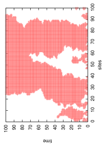
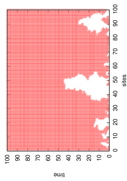
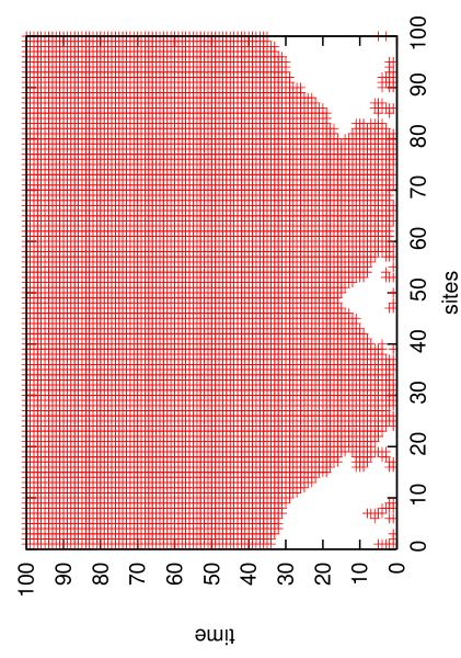
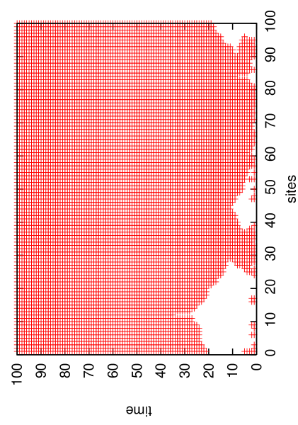
Figure 1: (Color online) Snapshots of the system in time for different values of $\beta=0.0,0.005,0.1$ and $\beta\to\infty$ (top to bottom) showing that for any non-zero $\beta$, the system equilibriates towards a homogeneous state much faster compared to the $\beta=0$ case. These snapshots are for a $L=100$ system.

In the simulations, we have generated systems of size $1000\leq L\leq 10000$ with a mininum of 1000 initial configurations for the maximum size in general. Only for $\beta=0$, the Ising limit, in which case the time taken to reach equilibrium is order of magnitude higher than that for any nonzero $\beta$, smaller systems have been simulated in some calculations. Depending on the system size and time to equilibriate, maximum iteration times have been set. Random sequential updating process has been used to control the spin flips.

On introducing $\beta$, we notice that well away from the Ising limit $\beta=0$, the dynamics gives $z\simeq 1.0$ and $\theta\simeq 0.235$ as in model I. However, as $\beta$ is made less than $O(10^{-1})$, the behaviour of the relevant dynamic quantities deviate from a simple power law behaviour. For example, the magnetisation shows an initial slow variation with time followed by a rapid growth before reaching saturation for values of $\beta<0.1$ (Fig. 2). It is difficult to fit a power law in either regime. This is true for the domain wall fraction decay as well (not shown). In fact, the rapid growth of magnetisation at later times is apparently even faster than $t^{1/2}$, that obtained for model I (e.g., for $\beta=0.001$). From the snapshots of the system for $\beta$ very close to zero, it is seen that for the first few steps the system has a behaviour similar to the Ising model ($\beta=0$). This explains the slow growth of magnetisation initially. However, as soon as a domain shrinks in size compared to its adjacent one, any non-zero $\beta$ makes it vanish very rapidly. However, it will be wrong to infer that the coersening process takes place faster than in model I, because in comparison, in model I, the system equilibriates in times much lesser than that for any finite $\beta$ (see Fig. 1).

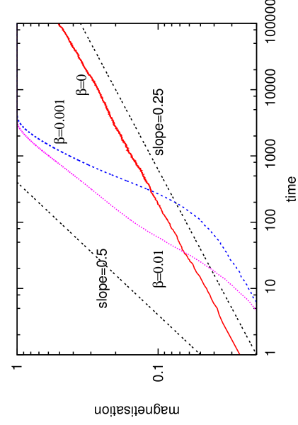
Figure 2: (Color online) Magnetisation as a function of time is shown for $\beta=0,0.001$ and $0.01$. The two starightlines in the log log plot have slopes corresponding to model I (0.5) and Ising model (0.25). The $\beta=0$ result is for $L=2000$ while the others are for $L=10000$.

The question remains therefore whether and how one can obtain an estimate of $z$ for $\beta\to 0$. Since a direct fitting fails, we try an indirect method. The average time $t_{eq}$ to reach the equilibrium state can be estimated from the time the magnetisation reaches a value unity. $t_{eq}$ is shown to scale as $L^{z}$ in Ising model with $z=2$ and for $\beta\to\infty$, $t_{eq}$ scales as $L^{z}$ with $z=1$ (inset of Fig. 3). Hence we plot $t_{eq}/L$ against $\beta$ for different $L$ and find an interesting result. For values of $\beta$ greater than 0.01, it shows a nice collapse, indicating $z=1$ here. As $\beta$ decreases, the deviation from a collapse starts appearing, it getting more pronounced for smaller values of $\beta$. However, at the same time, we notice that the deviation from a scaling $t_{eq}\propto L$ decreases for larger values of $L$ suggesting that the collapse as $\beta\to 0$ will improve with the system size. Thus we conclude that the exponent $z$ equals unity in the thermodynamic limit for any non-zero value of $\beta$. The deviations from the scaling as $\beta\to 0$ is simply a finite size effect.

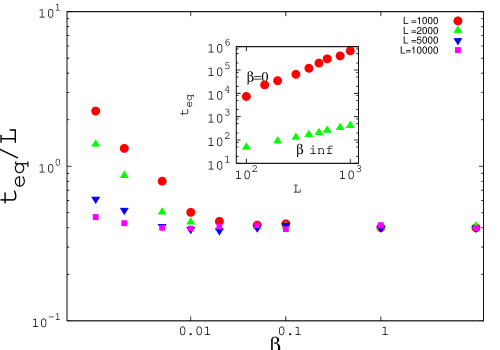
Figure 3: (Color online) The values of the time to equilibriate $t_{eq}$ scaled by the sytem size shows that for large $\beta$ there is a nice collapse. For small $\beta$, there are deviations from the collapse which decrease with the system size. Inset shows that $t_{eq}$ scales as $L^{z}$ for the limiting values $\beta=0$ with $z=2$ and for $\beta\to\infty$, $z=1$.

Hence from the above behaviour we conclude that the model I behaviour is valid for any finite $\beta$ and a dynamic transition takes place exactly at $\beta=0$.

Next we focus on the persistence data. Once again, as $\beta\to 0$, it is difficult to fit a unique power law to the persistence probability (Fig. 4). Here, in consistency with the magnetisation results, we find an initial decay of persistence quite fast and a late variation comparatively slower. The initial variation can be fitted to a power law and an estimate of $\theta$ made this way shows a tendency to continuously vary towards the $\beta=0$ value, i.e., 0.375. However, $\theta$ is not to be obtained from the early time behaviour and there is definitely a crossover to a different behaviour in later times before the persistence reaches saturation. Therefore determining $\theta$ from the initial variation is not a correct approach.

We even try to obtain a collapse by plotting $P(t)/t^{-\theta}$ against ${L/t^{z}}$ using trial values of $z$ and $\theta$ as in bcs ; biswas-sen , but for $\beta\to 0$, no collapse for large $L/t^{z}$, i.e., for small $t$, can be obtained, confirming once again that the determination of $\theta$ is not possible in a straightforward manner.

We next try to find out whether the scaling law $P_{sat}(L)\propto L^{-\alpha}$ is valid for finite values of $\beta$. When we plot the saturation values of persistence against different system sizes, we do find nice power law fittings and hence estimates of $\alpha$ can be made (Fig. 5). We find that $\alpha$ varies between $0.22$ and $0.23$ with no systematics indicating that it is independent of $\beta$. This once again supports the fact that there is a transition at $\beta=0$ as $\alpha$ has a known value (0.75) much larger for $\beta=0$.

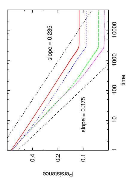
Figure 4: (Color online) The persistence probability against time is shown for different values of $\beta$ ($\beta=100,0.1,0.01$ and $0.005$ (from top to bottom); for small $\beta$ the slope cannot be uniquely determined. The two straightlines in the log log plot have slopes corresponding to the model I (0.235) and Ising model (0.375).

Although $\alpha$ shows no dependence on $\beta$, the saturation values of the persistence probability show an interesting dependence on $\beta$: for $\beta>>1$, it is independent of $\beta$ while for small values of $\beta$ it has a power law variation. We in fact find that the scaled variable $P_{sat}/{(\frac{\beta}{L}})^{\alpha}$ with $\alpha=0.225$ shows a collapse when plotted against $\beta$ suggesting a scaling form:

$$P_{sat}(L,\beta)=(\beta/L)^{\alpha}f(\beta).$$ (4)

The fact that for large values of $\beta$, the saturation values are independent of $\beta$ suggests that $f(\beta)$ varies as $\beta^{-\alpha}$ here. We indeed find this kind of a behaviour with $f(\beta)=constant$ for $\beta<<1$ and $f(\beta)\propto\beta^{-\alpha}$ for $\beta>>1$ (see inset of Fig. 5).

We thus find that the effect of the noise parameter $\beta$ is to cause a dynamic phase transition at $\beta=0$ showing that the behaviour of model I is indeed very robust. On the other hand, with respect to the Ising model, although the effect of noise is not comparable to thermal fluctuations as far as order-disorder transitions are concerned, it does induce a dynamic phase transition at $\beta=0$. The signature of the dynamical phase transition is seen in the variation of the dynamical quantities as the $\beta=0$ point is approached, there are also strong finite size effects.

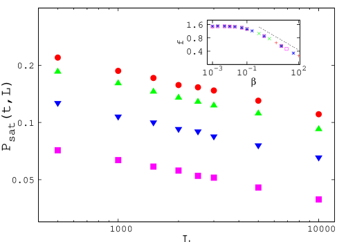
Figure 5: (Color online) The saturation values of the persistene probability shows a variation $L^{-\alpha}$ for values of $\beta=10.0,0.1,0.01$ and $0.001$ (from top to bottom) with $\alpha=0.225$. Inset shows that the scaled saturation values $P_{sat}/(\beta/L)^{\alpha}=f(\beta)$ varies as $\beta^{-\alpha}$ for large $\beta$.

One may raise the question as to what happens if $\beta$ is made negative. As expected, the system goes to a disordered state for any non-zero $\beta$ accompanied with exponential decay of persistence probability. In the spin picture, a negative value of $\beta$ does not correspond to any physical model, but in terms of domain wall movement, one has a system of mutually repulsive random walkers when $\beta<0$. The random walkers tend to move away from their nearest neighbours and therefore cannot annihilate each other but remain mobile all the time destroying the persistence of the spins. Such situations was seen to arise in spin systems like the ANNNI model annni also. The dynamic behaviour is therefore different for $\beta<0,\beta=0$ and $\beta>0$. So, allowing negative values of $\beta$, one may say that there is a dynamic phase transition occurring at $\beta=0$ separating three different dynamical phases.

Acknowledgment: Financial supports from DST grant no. SR-S2/CMP-56/2007 and discussions with P. Ray and S. Biswas are acknowledged.

References

- (1) S. Biswas and P. Sen, Phys Rev E 80 027101 (2009).
- (2) H. Hinrichsen, Adv. Phys. 49 815 (2000); J. Marro and R. Dickman, Nonequilibrium Phase Transitions in Lattice Models (Cambridge University Press, Cambridge), 1999; G. Odor, Rev. Mod. Phys. 76 663 (2004).
- (3) T. M. Liggett Interacting Particle Systems: Contact, Voter and Exclusion Processes (Springer-Verlag Berlin 1999).
- (4) D. Stauffer, in Encyclopedia of Complexity and Systems Science edited by R. A. Meyers (Springer, New York, 2009); K. Sznajd-Weron and J. Sznajd, Int. J. Mod. Phys C 11 1157 (2000); S. Galam, Int. J. Mod. Phys. C 19 409 (2008).
- (5) A. Baronchelli, L. Dall’Asta, A. Barrat, and V. Loreto, Phys. Rev. E 76, 051102 (2007); C. Castellano, M. Marsili and A. Vespignani, Phys. Rev. Lett. 85 3536 (2000).
- (6) J. Fuchs, J. Schelter, F. Ginelli and H. Hinrichsen, J. Stat. Mech. P04015 (2008).
- (7) D. Stauffer and P. M. C. de Oliveira, Eur. Phys. J B 30 587 (2002.)
- (8) J. R. Sanchez, arXiv:cond-mat/0408518v1
- (9) P. Shukla, J. Phys. A Math. Gen. 38 5441 (2005).
- (10) B. Derrida, A. J. Bray and C. Godreche, J.Phys. A 27 L357 (1994).
- (11) A. J. Bray, Adv. Phys. 43 357 (1994) and the references therein. For a review on persistence, see S. N. Majumdar, Curr. Sci. 77 370 (1999).
- (12) G. Manoj and P. Ray, Phys. Rev. E 62 7755 (2000); G. Manoj and P. Ray, J. Phys A 33 5489 (2000).
- (13) S. Biswas, A. K. Chandra and P. Sen, Phys. Rev. E 78, 041119 (2008)
- (14) P. K. Das, S. Dasgupta and P. Sen, J. Phys. A: Math. Theor. 40 6013 (2007).