Extracting strong measurement noise from stochastic series:
applications to empirical data

Abstract

It is a big challenge in the analysis of experimental data to disentangle the unavoidable measurement noise from the intrinsic dynamical noise. Here we present a general operational method to extract measurement noise from stochastic time series, even in the case when the amplitudes of measurement noise and uncontaminated signal are of the same order of magnitude. Our approach is based on a recently developed method for a nonparametric reconstruction of Langevin processes. Minimizing a proper non-negative function the procedure is able to correctly extract strong measurement noise and to estimate drift and diffusion coefficients in the Langevin equation describing the evolution of the original uncorrupted signal. As input, the algorithm uses only the two first conditional moments extracted directly from the stochastic series and is therefore suitable for a broad panoply of different signals. To demonstrate the power of the method we apply the algorithm to synthetic as well as climatological measurement data, namely the daily North Atlantic Oscillation index, shedding new light on the discussion of the nature of its underlying physical processes.

I Introduction

Recently, much effort has been made to uncover the dynamical process underlying a given time series of scale and time dependent complex systemsschreiberbook ; friedrich08 ; abarbanel93 . In many cases it is possible to describe such systems by a Langevin equation, extracted directly from the data, which separates the deterministic and stochastic processes inherent to the systemfriedrich97 . Such an approach has already been carried out successfully for instance for data from turbulent fluid dynamicsnawroth07 , financial datafriedrich00 , climate indicescollette04 ; lind05 and for electroencephalographic recordings from epilepsy patientsprusseit08 ; lehnertz09 and additional improvements were proposed to address the case of low sampling rateskleinhans05 ; gottschall08 .

However, typically the signal is subject to noise, due to experimental constraints or due to the measurement or discretization procedure leading to the data set to be studied. Such noise is not intrinsic to the system, differing from what is known as dynamical noise, and therefore one is interested to separate it from the stochastic process. We call such non-intrinsic noise measurement noise. To separate the measurement noise from the dynamics of the measured variable different predictor models or schemes for noise reduction may be usedschreiberbook ; abarbanel93 . In this context, an alternative procedure has been proposedboettcher06 to extract the intrinsic dynamics associated with Langevin processes strongly contaminated by measurement noise, based solely on the two conditional moments directly calculated from the datagottschall08 ; boettcher06 .

In this manuscript we will revisit this nonparametric procedure, describing it in detail and explaining the main steps for its implementation, with the aim of applying it to empirical data sets. Let us consider a one-dimensional Langevin process $x(t)$ (an extension to more dimensions is straightforward) defined as

$$\frac{dx}{dt}=D_{1}(x)+\sqrt{D_{2}(x)}\Gamma_{t},$$ (1)

where $\Gamma_{t}$ represents a Gaussian $\delta$-correlated white noise $\langle\Gamma_{t}\rangle=0$ and $\langle\Gamma_{t}\Gamma_{t^{\prime}}\rangle=\delta(t-t^{\prime})$. Functions $D_{1}(x)$ and $D_{2}(x)$ are the drift and diffusion coefficients defined as

$$D_{n}(x)=\frac{1}{n!}\lim_{\tau\to 0}\frac{1}{\tau}{M}_{n}(x,\tau)$$ (2)

for $n=1,2$, where ${M}_{n}(x,\tau)$ denotes the $n$-th order conditional moment of the data, as explained below. Further, we consider that $x(t)$ is ‘contaminated’ by a Gaussian $\delta$-correlated measurement white noise, which leads to the series of observations

$$y(t)=x(t)+\sigma\zeta(t)$$ (3)

where $\sigma$ denotes the amplitude of the measurement noise.

When there is no measurement noise ($\sigma=0$), Eq. (3) yields the particular case $y(t)\equiv x(t)$, and the evolution equation underlying the signal can be extracted directly from the two conditional moments ($n=1,2$)

$$\hat{M}_{n}(y_{i},\tau) = \langle(y(t+\tau)-y(t))^{n}\rangle|_{y(t)=y_{i}}$$ (4)

as described in Refs. friedrich97 ; friedrich00 ; lind05 ; boettcher06 .

In the presence of measurement noise ($\sigma\neq 0$) the conditional moments depend on $x$, $\tau$ and $\sigma$. Since generally the limit

$$\lim\limits_{\tau\to 0}\hat{M}_{n}(x,\sigma\neq 0,\tau)$$ (5)

does not exist, Eq. (3) cannot be applied. The aim of this paper, however, is to explicitly derive a procedure which can transform the functional form of the ’noisy conditional moments’ $\hat{M}_{1}(x,\sigma,\tau)$ and $\hat{M}_{2}(x,\sigma,\tau)$ at small $\tau$ into the ’true’ coefficients $D_{1}(x)$ and $D_{2}(x)$ and simultaneously retrieve the amplitude $\sigma$ of the associated measurement noise. For that, we show that $\hat{M}_{n}(y,\tau)$ for fixed $y$ is typically linear in $\tau$ for a certain range $[\tau_{1},\tau_{2}]$ of values (see Fig. 4 below). Therefore, even when $\sigma\neq 0$ one can estimate the quantities

$$\hat{D_{n}}(y)=\frac{\hat{M}_{n}(y,\tau_{2})-\hat{M}_{n}(y,\tau_{1})}{n!(\tau_{2}-\tau_{1})}.$$ (6)

We start in Sec. II by briefly describing the procedure to extract Langevin equations from data sets and show how the drift and diffusion coefficients depend on the measurement noise strength $\sigma$. In particular, we will see that the proposed estimatesiefert03 does not yield the correct value when the measurement noise is too strong. In Sec. III we then proceed to minimize a proper least square function using the Levenberg-Marquardt procedurenumrecip . By applying this algorithm to synthetic data we show that indeed this approach is able to reliably extract the noise amplitude even in cases where it is of the same order as the synthetic signal without noise. Furthermore, the procedure yields simultaneously more accurate estimates for the clean signal $x(t)$. Finally, in Sec. IV, we apply this framework to an empirical data set, namely the North Atlantic Oscillation daily indexijbc , giving some insight from the obtained results to the underlying system. Discussion and conclusions are given in Sec. V, where further possible applications are proposed. All details concerning the implementation of the minimization procedure to extract strong measurement noise are given as appendices.

II Stochastic time series with strong measurement noise

We consider a time series generated by integrating Eq. (1) with drift and diffusion coefficient assumed to be linear and quadratic forms respectively

$$D_{1}(x) = d_{10}+d_{11}x$$ (7a)

$$D_{2}(x) = d_{20}+d_{21}x+d_{22}x^{2},$$ (7c)

and by adding separately to each data point the measurement term $\sigma\zeta(t)$ in Eq. (3). Though we concentrate on the particular expressions for $D_{1}$ and $D_{2}$ given above, it should be stressed that they comprehend a large collection of different processes, such as Ornstein-Uhlenbeck processesboettcher06 . Further, some generalizations may be carried out as will be discussed in Sec. V. Using Eqs. (7a) and (7b), one has six parameters: five coefficients $d_{ij}$ defining the evolution equation of the clean signal and a sixth parameter $\sigma$ for the amplitude of the measurement noise.

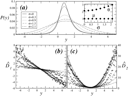
Figure 1: Langevin time series with different measurement noise strengths. Here we show (a) the probability density function $P(y)$ of the series with noise (see Eq. (3)), with the corresponding mean value $\mu$ and standard deviation $\theta$ in the inset, and the corresponding functions (b) ${\hat{D}}_{1}(y)$ and (c) ${\hat{D}}_{2}(y)$, see Eq. (6). In all cases, the assumed time series $x(t)$ without measurement noise uses the coefficients $D_{1}(x)=1-x$ and $D_{2}(x)=1-x+x^{2}$.

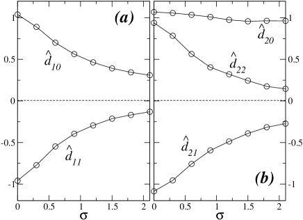
Figure 2: Noise dependence of functions $\hat{D}_{1}(y)$ and $\hat{D}_{2}(y)$ (see text and Eq. (6)) The underlying Langevin time series $x(t)$ without noise is the same as in Fig. 1.

Figure 1 illustrates this influence of noise for a particular choice of $D_{1}(x),D_{2}(x)$. As shown in Fig. 1a, for increasing $\sigma$ one obtains broader probability density functions $P(y)$ as one intuitively expects. Quantitatively, the standard deviation $\theta$ of $P(y)$ varies quadratically with the measurement noise $\sigma$, while the mean value $\mu$ of $P(y)$ remains constant, as shown in the inset of Fig. 1a. The estimated functions $\hat{D}_{1}(y)$ and $\hat{D}_{2}(y)$ change significantly, as shown in Fig. 1b and 1c respectively. Assuming ${\hat{D}}_{1}(y)={\hat{d}}_{10}+{\hat{d}}_{11}y$ and ${\hat{D}}_{2}(y)={\hat{d}}_{20}+{\hat{d}}_{21}y+{\hat{d}}_{22}y^{2}$, Fig. 2 shows how the estimated parameters $\hat{d}_{ij}$ deviate from the ‘true’ uncontaminated values $d_{ij}$ in Eq. (7) when measurement noise increases. Notice that for $\sigma=0$ – see left vertical axis in the plots of Fig. 2 – the estimated parameter values are approximately correct.

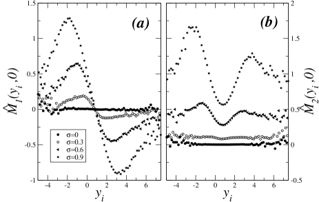
Figure 3: Conditional moments ${\hat{M}}_{1}(y_{i},\tau)$ and ${\hat{M}}_{2}(y_{i},\tau)$ as a function of bin $y_{i}$, for $\tau=0$ and different measurement noise strengths. The asymmetry of ${\hat{M}}_{2}$ is due to $d_{21}\neq 0$ (see Eqs. (7)). The same $x(t)$ as in Fig. 1 was used.

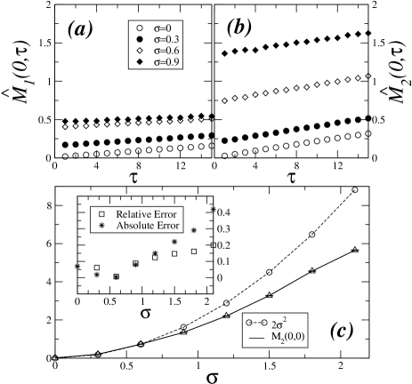
Figure 4: Conditional moments (a) ${\hat{M}}_{1}(y_{i},\tau)$ and (b) ${\hat{M}}_{2}(y_{i},\tau)$ as a function of $\tau$, for bin $y_{i}=0$ and different measurement noise strengths. In (c) one compares the true measurement noise with the approximation $\sigma_{app}={\hat{M}}_{2}(0,0)\sim 2\sigma^{2}$ given in Eq. (9). In the inset the corresponding absolute and relative erros are given by $\zeta_{a}=|\sigma-\sigma_{app}|$ and $\zeta_{r}=\zeta_{a}/\sigma$ respectively. Errors for $\hat{M}_{2}$ are negligible. The same $x(t)$ as in Fig. 1 was used.

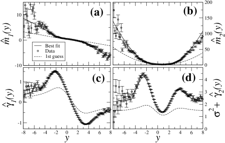
Figure 5: Functions $\hat{m}_{1}$, $\hat{m}_{2}$, $\hat{\gamma}_{1}$ and $\hat{\gamma}_{2}$ (symbols) defining the conditional moments in Eqs. (8). The underlying Langevin time series $x(t)$ without noise is characterized by a drift coefficient $D_{1}(x)=1-x$ and a diffusion coefficient $D_{2}(x)=1-x+x^{2}$. The measurement noise was fixed at $\sigma=1$. Each hat-function is compared with the corresponding integral form in Eqs. (10) using the first estimate of parameters values (dashed lines) and the true values (solid lines).

To correctly derive the drift and diffusion coefficients $D_{1}(x)$ and $D_{2}(x)$ when $\sigma$ is strong, we consider the measured conditional moments $\hat{M}_{1}(y_{i},\tau)$ and $\hat{M}_{2}(y_{i},\tau)$, as in Eq. (4), the hat indicating that they are calculated from the measured data $y(t)$ directly. Since this conditional moments depend in a non trivial way on both time $\tau$ and amplitude $y_{i}$, we approximate them up to first order on $\tau$:

$$\hat{M}_{1}(y_{i},\tau) = \langle y(t+\tau)-y(t)\rangle|_{y(t)=y_{i}}$$ (8a)

$$= \tau\hat{m}_{1}(y_{i})+\hat{\gamma}_{1}(y_{i})+{\cal O}(\tau^{2}),$$ (8c)

$$\hat{M}_{2}(y_{i},\tau) = \langle(y(t+\tau)-y(t))^{2}\rangle|_{y(t)=y_{i}}$$ (8e)

$$= \tau\hat{m}_{2}(y_{i})+\hat{\gamma}_{2}(y_{i})+\sigma^{2}+{\cal O}(\tau^{2}),$$ (8g)

where $y(t)$ is taken in the range $y_{i}\pm\Delta y/2$ for each bin $i$, and $\Delta y$ depends on the binning considered. Appendix A gives the full derivation of Eqs. (8).

Figure 3 shows both conditional moments for $\tau=0$ and with different measurement noise strengths. Conversely, in Fig. 4a and 4b one sees that the conditional moments depend linearly on $\tau$ for a fixed amplitude $y$, which justifies the approximation assumed in Eqs. (8). Therefore, to study the dependence of the conditional moments on $y$ we will consider the linear decompositions in Eqs. (8), as done in Fig. 5. Our simulations with synthetic data have shown that using a to large range of $\tau$ values yields results for $D_{1}$ and $D_{2}$ deviated from their true values. The best estimation for both Kramers-Moyal coefficients are obtained using the range $1<\tau\lesssim 4$.

Notice that for sufficiently small measurement noise a good estimate of it is given byboettcher06 ; siefert03

$$\sigma\approx\sqrt{\frac{\hat{M}_{2}(\mu,0)}{2}},$$ (9)

where $\mu$ is the average value of $y(t)$ data points in the time series. For details see Append. A. However, as shown in Fig. 4c, this approximation is no longer valid for sufficiently high measurement noise, namely when $\sigma\gtrsim 0.5$ (see inset of Fig. 4c) and even otherwise coefficients $D_{1}$ and $D_{2}$ are not correctly estimated (see Fig. 2). Therefore, a better algorithm to estimate such parameters is necessary.

The heart of our procedure to correctly estimate measurement noise lies in the fact that while the functions $\hat{m}_{i}$ and $\hat{\gamma}_{i}$ (i=1,2) are obtained explicitly for each bin value $y_{i}$, functions $m_{i}$ and $\gamma_{i}$ depend generally on the drift and diffusion coefficients as follows:

$$\gamma_{1}(y) = \int_{-\infty}^{+\infty}(x-y)\bar{f}_{\sigma}(x|y)dx$$ (10a)

$$\gamma_{2}(y) = \int_{-\infty}^{+\infty}(x-y)^{2}\bar{f}_{\sigma}(x|y)dx$$ (10c)

$$m_{1}(y) = \int_{-\infty}^{+\infty}D_{1}(x)\bar{f}_{\sigma}(x|y)dx$$ (10e)

$$m_{2}(y) = 2\int_{-\infty}^{+\infty}[(x-y)D_{1}(x)+D_{2}(x)]\bar{f}_{\sigma}(x|y)dx,$$ (10g)

where $\bar{f}_{\sigma}(x|y)$ is the probability for the system to adopt the value $x$ when a measured value $y$ is observed. For details about the derivation of functions in Eqs. (10) see Append. A and for the explicit expression of $\bar{f}_{\sigma}(x|y)$ see Append. B.

In Fig. 5 we illustrate both the hat-functions in Eqs. (8) and their integral form in Eqs. (10). Due to the measurement noise fixed in this example at $\sigma=1$ the hat-functions (symbols) are not properly fitted by the integral form in Eqs. (10) using the first estimate (dashed lines) of the parameters $d_{ij}$, taken from Fig. 2, and $\sigma$, computed from Eq. (9). If instead we use the true parameter values in the integral forms of our $m_{i}$ and $\gamma_{i}$ functions a proper fit is obtained (solid lines).

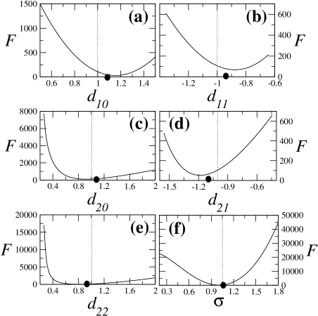
Figure 6: Function $F$ in Eq. (17) as a function of (a) $d_{10}$, (b) $d_{11}$, (c) $d_{20}$, (d) $d_{21}$, (e) $d_{22}$ and (f) $\sigma$. The same situation as in Fig. 2 is here chosen: $D_{1}(x)=1-x$, $D_{2}(x)=1-x+x^{2}$ and $\sigma=1$. Dashed lines indicate the true values used for generating the data series, while the bullet indicates the estimated values of the Kramers-Moyal coefficients for $\sigma=0$. In each plot while varying one parameter, the remaining ones are fixed at their true values (see text).

Therefore, the problem we want to solve is to determine the parameters that minimize the function:

$$F = \frac{1}{M}\sum_{i=1}^{M}\Big{[}\frac{\left(\hat{\gamma}_{1}-\gamma_{1}(y_{i})\right)^{2}}{\sigma^{2}_{\hat{\gamma}_{1}}(y_{i})}+$$ (17)

$$\phantom{\frac{1}{M}\sum_{i=1}^{M}\Big{[}}\frac{\left(\hat{\gamma}_{2}-\gamma_{2}(y_{i})-\sigma^{2}\right)^{2}}{\sigma^{2}_{\hat{\gamma}_{2}}(y_{i})}+$$

$$\phantom{\frac{1}{M}\sum_{i=1}^{M}\Big{[}}\frac{\left(\hat{m}_{1}-m_{1}(y_{i})\right)^{2}}{\sigma^{2}_{\hat{m}_{1}}(y_{i})}+$$

$$\phantom{\frac{1}{M}\sum_{i=1}^{M}\Big{[}}\frac{\left(\hat{m}_{2}-m_{2}(y_{i})\right)^{2}}{\sigma^{2}_{\hat{m}_{2}}(y_{i})}\Big{]},$$

where the summation extends over all $M$ bins, $\sigma_{\hat{\gamma}_{1}}(y_{i})$ is the error associated to function $\hat{\gamma}_{1}$ at the value $y_{i}$ and similarly for $\sigma_{\hat{\gamma}_{2}}$, $\sigma_{\hat{m}_{1}}$ and $\sigma_{\hat{m}_{2}}$. Notice that the values of such $\sigma_{\hat{\gamma}_{i}}$ and $\sigma_{\hat{m}_{i}}$ are taken directly from the data only. See Appendix A for details.

Taking again the example illustrated in Fig. (2) with $\sigma=1$ we plot in Fig. 6 function $F$ in Eq. (17) as function of each one of the parameters keeping all others fixed at their true values. Evidently, the estimated values are near the minimum of $F$ in each case. Further, the one-dimensional cuts of function $F$ show only one minimum. One should note however that, for the entire $6$-dimensional parameter space, several local minima of $F$ may appear. In fact, after minimizing $F$ by varying one parameter, function $F$ also changes as a function of the other parameters, i.e. its minimum as a function of the other parameter changes. In the next Section we will see how to minimize function $F$, in order to find good estimates for the correct values for each parameter.

III Optimization procedure

After computing the functions $\hat{\gamma}_{1}$, $\hat{\gamma}_{2}$, $\hat{m}_{1}$ and $\hat{m}_{2}$ as well as the corresponding errors $\sigma_{\hat{\gamma}_{1}}$, etc, directly from the measured time series $y(t)$ and estimating the coefficients $D_{1}$ and $D_{2}$ given by the functional forms in Eqs. (7) there are several ways to minimize $F$. All of them start from the initially estimated set of values for the parameters and iteratively improve the solution, by finding lower values of $F$, till convergence is attained.

To proceed the following remark should be considered. Parameter $d_{10}$ can be always eliminated with a simple transformation $x\to x^{\prime}=x+d_{10}/d_{11}$. Alternatively, and since we do not know beforehand the true values of $d_{10}$ and $d_{11}$ we can consider also the fact that averaging Eq. (1) yields $d_{10}=-d_{11}\langle x\rangle$ and consider the transformation $x^{\prime}=x-\langle x\rangle$. With these arguments, we henceforth disregard $d_{10}$, which reduces the dimension of parameter space by one. Parameter $d_{10}$ is computed from the relations above, only after minimizing $F$. For simplicity the primes in $x^{\prime}$ will be omitted.

The simplest way is to minimize each term in $F$ and repeat that a large number of times starting from different initial conditions for the parameters, in a sort of a Monte Carlo procedure of random walks bouchaud90 or Lévy-walksmetzler00 . The Monte Carlo procedure assures that a substantial number of local minimal for $F$ will be visited, and in the end we take the minimum of all $F$ values found. Simulations have shown however that a Monte Carlo procedure is too expensive in this case, since there are different local minima and the choice of the minimum is strongly path dependent. We will therefore consider the Levenberg-Marquardt methodnumrecip .

For the Levenberg-Marquardt procedure one computes the first and second derivative of $F$. Symbolizing the parameters $\sigma,d_{11},d_{20},d_{21}$ and $d_{22}$ by $p_{k}$ with $k=1,\dots,5$ respectively, these derivatives read

$$\frac{\partial F}{\partial p_{k}} = -\frac{2}{M}\sum_{i=1}^{M}\Big{[}\frac{\hat{\gamma}_{1}-\gamma_{1}}{\sigma^{2}_{\hat{\gamma}_{1}}(i)}\frac{\partial\gamma_{1}}{\partial p_{k}}+\frac{\hat{\gamma}_{2}-\gamma_{2}-\sigma^{2}}{\sigma^{2}_{\hat{\gamma}_{2}}(i)}\frac{\partial(\gamma_{2}+\sigma^{2})}{\partial p_{k}}+\frac{\hat{m}_{1}-m_{1}}{\sigma^{2}_{\hat{m}_{1}}(i)}\frac{\partial m_{1}}{\partial p_{k}}+\frac{\hat{m}_{2}-m_{2}}{\sigma^{2}_{\hat{m}_{2}}(i)}\frac{\partial m_{2}}{\partial p_{k}}\Big{]},$$ (18)

$$\frac{\partial^{2}F}{\partial p_{k}\partial p_{\ell}} = \frac{2}{M}\sum_{i=1}^{M}\Big{[}\frac{1}{\sigma^{2}_{\hat{\gamma}_{1}}(i)}\frac{\partial\gamma_{1}}{\partial p_{k}}\frac{\partial\gamma_{1}}{\partial p_{\ell}}-\frac{\hat{\gamma}_{1}-\gamma_{1}}{\sigma^{2}_{\hat{\gamma}_{1}}(i)}\frac{\partial^{2}\gamma_{1}}{\partial p_{k}\partial p_{\ell}}+$$ (27)

$$\phantom{\frac{2}{M}\sum_{i=1}^{M}\Big{[}}\frac{1}{\sigma^{2}_{\hat{\gamma}_{2}}(i)}\frac{\partial(\gamma_{2}+\sigma^{2})}{\partial p_{k}}\frac{\partial(\gamma_{2}+\sigma^{2})}{\partial p_{\ell}}-\frac{\hat{\gamma}_{2}-\gamma_{2}-\sigma^{2}}{\sigma^{2}_{\hat{\gamma}_{2}}(i)}\frac{\partial^{2}(\gamma_{2}+\sigma^{2})}{\partial p_{k}\partial p_{\ell}}+$$

$$\phantom{\frac{2}{M}\sum_{i=1}^{M}\Big{[}}\frac{1}{\sigma^{2}_{\hat{m}_{1}}(i)}\frac{\partial m_{1}}{\partial p_{k}}\frac{\partial m_{1}}{\partial p_{\ell}}-\frac{\hat{m}_{1}-m_{1}}{\sigma^{2}_{\hat{m}_{1}}(i)}\frac{\partial^{2}m_{1}}{\partial p_{k}\partial p_{\ell}}+\frac{1}{\sigma^{2}_{\hat{m}_{2}}(i)}\frac{\partial m_{2}}{\partial p_{k}}\frac{\partial m_{2}}{\partial p_{\ell}}-\frac{\hat{m}_{2}-m_{2}}{\sigma^{2}_{\hat{m}_{2}}(i)}\frac{\partial^{2}m_{2}}{\partial p_{k}\partial p_{\ell}}\Big{]}$$

$$\sim \frac{2}{M}\sum_{i=1}^{M}\Big{[}\frac{1}{\sigma^{2}_{\hat{\gamma}_{1}}(i)}\frac{\partial\gamma_{1}}{\partial p_{k}}\frac{\partial\gamma_{1}}{\partial p_{\ell}}+\frac{1}{\sigma^{2}_{\hat{\gamma}_{2}}(i)}\frac{\partial(\gamma_{2}+\sigma^{2})}{\partial p_{k}}\frac{\partial(\gamma_{2}+\sigma^{2})}{\partial p_{\ell}}+$$ (33)

$$\phantom{\frac{2}{M}\sum_{i=1}^{M}\Big{[}}\frac{1}{\sigma^{2}_{\hat{m}_{1}}(i)}\frac{\partial m_{1}}{\partial p_{k}}\frac{\partial m_{1}}{\partial p_{\ell}}+\frac{1}{\sigma^{2}_{\hat{m}_{2}}(i)}\frac{\partial m_{2}}{\partial p_{k}}\frac{\partial m_{2}}{\partial p_{\ell}}-2\delta_{\sigma p_{k}}\delta_{\sigma p_{\ell}}\frac{\hat{\gamma}_{2}-\gamma_{2}-\sigma^{2}}{\sigma^{2}_{\hat{\gamma}_{2}}(i)}\Big{]}.$$

In the right-hand side of Eq. (33) we neglect the terms containing second derivatives of $\gamma$ and $m$ functions. This last approximation of neglecting second derivatives is acceptable as far as the model is successfulnumrecip .

By symbolizing first and second derivatives as $\beta_{k}$ and $\alpha_{k\ell}$ respectively the iterative procedure computes the increments $dp_{k}$ for each parameter $p_{k}$ ($k=1,\dots,5$), which are the solutions of

$$\beta_{k}=-\sum_{\ell=1}^{5}\alpha_{k\ell}dp_{\ell}.$$ (34)

Furthermore, one assumes that $dp_{\ell}\propto\beta_{\ell}$, which considering dimensional analysisnumrecip can be written as:

$$dp_{\ell}=\frac{\beta_{\ell}}{\lambda\alpha_{\ell\ell}},$$ (35)

where typically $\lambda\gg 1$. For a given $\lambda$ value, instead of the second derivatives $\alpha_{mn}$ one assumes $\alpha^{\prime}_{mn}=\alpha_{mn}(1+\lambda)$ for $m=n$ and $\alpha^{\prime}_{mn}=\alpha_{mn}$ otherwise and solves Eq. (34) for $dp_{k}$ numrecip .

If $F(p_{k}+dp_{k})<F(p_{k})$, the parameter values are updated, $p_{k}\to p_{k}+dp_{k}$, and $\lambda$ is typically decreased by $10\%$. Otherwise, if $F(p_{k}+dp_{k})\geq F(p_{k})$ one increases $\lambda$ by $10\%$ and determines new increments $dp_{k}$. The procedure stops after attaining the required convergence.

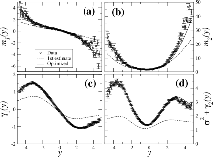
Figure 7: Functions $m_{1}$, $m_{2}$, $\gamma_{1}$ and $\gamma_{2}$ for the Langevin process with $D_{1}(x)=1-x$, $D_{2}(x)=1-x+x^{2}$ and $\sigma=1$. Symbols indicate the functions obtained for the data, dashed line corresponds to the first estimate of the parameters and solid line corresponds to the parameter values obtained from the Levenberg-Marquardt procedure (see text). In this case, for the first estimate one has $F_{0}=3720$ while the final estimate retrieves $F_{LM}=33.1$. The true minimum is $F_{m}=29.2$.

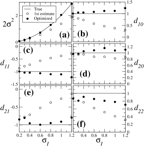
Figure 8: Comparison of the optimized parameters values (bullet) with the first estimate and the true values for different input measurement noise strengths $\sigma_{I}$: (a) $2\sigma^{2}$, (b) $d_{10}$, (c) $d_{11}$, (d) $d_{20}$, (e) $d_{21}$, (f) $d_{22}$. The measurement noise is correctly extracted as well as the parameters defining the drift coefficient $D_{1}(x)$ which controls the deterministic part of the underlying evolution equation (see text).

Using the same data as generated in Fig. 5 with $\sigma=1$, we now plot in Fig. 7 the functions $\hat{m}_{i}$ and $\hat{\gamma}_{i}$ for the data (symbols) and compare them with the integral forms of those functions for the first estimate of parameter values (dashed lines) and the optimized solution obtained with the Levenberg-Marquardt procedure (solid lines). Clearly, the optimized functions fit better the data and the minimum of $F$ found is very close to its true value (see caption of Fig. 7).

Notice that the optimized values $d_{ik}^{\prime}$ are obtained for the transformed data ($x\to x^{\prime}=x-\langle x\rangle$), assuming $d_{10}^{\prime}=0$. In practice one obtains $d_{10}^{\prime}\sim 10^{-2}$, typically two orders of magnitude smaller than the other coefficients. Using $\langle x\rangle=-d_{10}/d_{11}$, one obtains the true coefficients according to $d_{10}=-d_{11}^{\prime}\langle x\rangle$, $d_{11}=d_{11}^{\prime}$, $d_{20}=d_{20}^{\prime}-d_{21}^{\prime}\langle x\rangle+d_{22}^{\prime}\langle x\rangle^{2}$, $d_{21}=d_{21}^{\prime}-2d_{22}^{\prime}\langle x\rangle$ and $d_{22}=d_{22}^{\prime}$.

To show the power of the present procedure we next generate several synthetic data sets from Eq. (1) with different measurement noise amplitudes $\sigma_{I}$ in the range $[0,1.2]$. The same $D_{1}(x)$ and $D_{2}(x)$ as in Fig. 2 is used. Results are shown in Fig. 8. The circles indicate the obtained parameter values for the first estimate, as in Fig. 2. The solid lines indicate the true values used to generate the data, while bullets indicate the value after optimization.

From Fig. 8a one sees that after optimization the value of $\sigma_{I}$ is always correctly determined. Such finding is of major importance and shows the relevance of our approach for practical applications even for strong measurement noise, since the uncontaminated series $x$ typically lies within the range $[-2,2]$, having therefore values close to the amplitude $\sigma_{I}$ of the measurement noise.

Figures 8b and 8c also show a very reliable estimate for the two parameters $d_{10}$ and $d_{11}$ respectively, defining the drift coefficient $D_{1}(x)$. Since this coefficient characterizes the deterministic part of the evolution equation for $x$, this accurate estimate should provide valuable insight into the dynamics of the underlying system.

As for the diffusion coefficient $D_{2}(x)$, Figs. 8d-f show that the estimate of $d_{22}$ is no longer as good as for the other parameters. Parameter $d_{20}$ is reasonably estimated but the optimized estimate is as good as the first one.

For stronger measurement noise, namely for $\sigma>1.2$, one faces the problem that the optimization procedure is sometimes stucked in a local minimum of the function $F$ leading to unreliable coefficients $d_{ik}$. This is in principle a shortcoming of the presently used minimization algorithm. In addition, the function $F$ itself is based on estimated functions $m$ and $\gamma$ and therefore itself subject to errors. A forthcoming study will address the observed issues in the context of global optimization.

IV The North Atlantic Oscillation: an empirical example

In this section we apply our framework to the North Atlantic Oscillation daily index, which presents data with strong measurement noise. Table 1 summarizes the optimized values for all parameter describing the data set, comparing it with simulations.

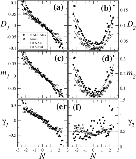
Figure 9: (a)-(b) Estimate of the drift and diffusion coefficients $D_{1}(N)$ and $D_{2}(N)$ of the daily North Atlantic Index $N$ijbc ($16801$ datapoints), together with the corresponding (c) $m_{1}(N)$, (d) $m_{2}(N)$, (e) $\gamma_{1}(N)$ and (f) $\gamma_{2}(N)$. Results for the empirical NAO index are represented with bullets whereas the synthetic data also with $16801$ datapoints and parameter values given by Tab. 1 is shown with circles for comparison. The corresponding fits are given with solid and dashed lines, respectively.

The North Atlantic Oscillation (NAO) is a source of variability in the global atmosphere, describing a large-scale vacillation in atmospheric mass between the anticyclone near the Azores and the cyclone near Iceland hurrel95 . The state of the NAO is usually measured by an index $N$, defined as the normalized pressure difference between the high and the low poles, where the pressures are averaged over each, day, month or year lind05 ; hurrel95 . The NAO index and climate indices in general are receiving much attention due to their important role in climate change. Lately, evidences for the stochasticity of this index have been showncollette04 ; lind05 . In this section we address the problem of estimating its measurement noise amplitude.

Figures 9a and 9b show the drift and diffusion coefficients respectively for the NAO daily index (bullets) and the corresponding fit (solid line). The parameters $d_{ij}$ for both $D_{1}$ and $D_{2}$ are given in Tab. 1 together with the amplitude of the measurement noise. Probably due to the small amount of data points ($16\ 801$ values) one observes large scattering of the data, particularly away from the average value $\langle N\rangle\sim 0$.

To evaluate the reliability of considering the NAO index a Markov process described by Eq. (1) we also plot in Figs. 9 the results obtained when integrating such equation (circles) using the coefficient values in Tab. 1 including the amplitude of the measurement noise. The same sample size was considered. The corresponding fit is represented with a dashed line. While the drift coefficient $D_{1}$ resembles the one observed for the NAO index, there is a significant shift of the diffusion coefficient, that only for a very narrow range around the average value is well reproduced. Indeed, as one sees from Tab. 1, the coefficient values for $D_{2}$ in our simulation significantly deviate from the ones found for the NAO series.

Further, functions $m_{i}$ and $\gamma_{i}$, plotted in Figs. 9c-f, show also large scattering, particularly for $\gamma_{2}$. This feature raises difficulties in a proper minimum search for $F$.

Param.		Simulations (16801 pts, 10 sim)
	NAO Index
	(16801 pts)	With noise	No noise	Only noise
$\mathbf{\sigma}$ ($\times 10^{-3}$)	$455$	$455\pm 34$	$106\pm 17$	$321\pm 9$
$\mathbf{d_{10}}$ ($\times 10^{-3}$)	$-2.6$	$-3.1\pm 0.5$	$-3.8\pm 0.1$	$10^{-6}\pm 10^{-2}$
$\mathbf{d_{11}}$ ($\times 10^{-3}$)	$-40$	$-24\pm 9$	$-29\pm 2$	$0.1\pm 1$
$\mathbf{d_{20}}$ ($\times 10^{-3}$)	$39$	$24\pm 1$	$29\pm 0.1$	$0.1\pm 1$
$\mathbf{d_{21}}$ ($\times 10^{-3}$)	$1.5$	$-0.3\pm 1$	$-1.6\pm 0.2$	$0.1\pm 1$
$\mathbf{d_{22}}$ ($\times 10^{-3}$)	$16$	$13\pm 3$	$11\pm 0.5$	$-1\pm 7$

Table 1: Optimized parameter values for the daily North Atlantic Oscillation daily indexijbc compared with the average values for $10$ sets of synthetic data (“With noise”) using the same number of points and parameter values. In order to evaluate the reliability of our synthetic data we also run the optimization procedure for $10$ sets of synthetic data with the same $D_{1}$ and $D_{2}$ found in NAO series and $\sigma=0$ (“No noise”). In the last column we plot the results returned from the optimization procedure for synthetic data of pure measurement noise with amplitude $\sigma=0.455$, the one obtained for NAO series.

In order to check the reliability of the calculations we reproduce the synthetic data $10$ times and present in Tab. 1 (column “With noise”) the average values for each parameter, where the error is taken as the largest deviation from the average over the sample of data sets. The measurement noise, which dominates all parameters, is well reproduced. For the drift and diffusion coefficient the order of magnitude of each parameter is also correct, but for $d_{11}$ and and $d_{20}$ one observes significant deviations from the estimated values obtained for the NAO series.

This mismatch between the empirical and synthetic series could raise the question if the NAO Index is indeed suitably described by a Markovian stochastic process with a perceivable deterministic part. In fact, since one observes $\sigma\gg d_{ij}$ the series is approximately a pure white noise (i.e. $y(t)=\sigma\zeta(t)$ in Eq. (3)), which in fact also yields a linear drift and quadratic diffusion coefficients.

To address this problem we rerun our optimization procedure for synthetic data, for two additional situations, one where $\sigma=0$ and drift and diffusion coefficients are given by the NAO index, and another one which simulates a pure white noise ($D_{1}=D_{2}=0$) with $\sigma$ equal to the value found for the NAO series. The results are also given in Tab. 1, columns “No Noise” and “Only noise” respectively.

For the pure white noise process one obtains $\sigma$ as the only non-zero parameter, apart fluctuations, but with an amplitude different from the one used to generate the synthetic data, namely $\sigma\simeq 0.321$, which corresponds to $\sim 75\%$ of the inserted measurement noise ($\sigma=0.445$). For the synthetic process with no noise, the order of magnitude for the parameters of $D_{1}$ and $D_{2}$ is correctly computed, whereas a non-zero measurement noise is retrieved covering the remaining $25\%$ of the inserted measurement noise. In other words, one can argue that in this situation our procedure retrieves $\sim 75\%$ of the total amount of measurement noise.

In this scope, our results point in the direction of previous arguments given by some authorsstephenson00 : differently from other climate indices such as the ENSO index, the NAO index seems to be an almost pure white noise process with only a minor contribution from a stochastic process governed by a Langevin-like equation. Alternative indices should be therefore considered and studied as recently suggestedlind05 .

V Discussion and Conclusions

We described in detail a nonparametric procedure to extract measurement noise in empirical stochastic series with strong measurement noise. The algorithm is able to accurately extract the strength of measurement noise and the values of the parameters defining the drift coefficient and to estimate with good accuracy the diffusion coefficient that fully describe the evolution equation for the measured quantity in the time series. This has been shown by synthetically generated data sets contaminated by increasing measurement noise. Additionally, the algorithm was applied to a set of measured data providing new insight in the underlying systems. The data for the climate index shows a large scattering, probably due to the small amount of data points. Larger data sets for climate indices are not available up to our knowledge.

It should be noticed that the nonparametric reconstruction of the Langevin Eq. (1) from measured stationary data sets generally requires that the process exhibits Markovian properties and fulfils the Pawula theoremlind05 . While the second constraint can be relaxed extending the analysis to a broader class of Langevin-like systems in which the Gaussian $\delta$-correlated white noise Langevin force is replaced by a more general Lévy noisefriedrich08 ; siegert01 , in general the Markov condition remains a crucial constraint.

Recently, it has been shown that processes corrupted from measurement noise may loose their Markov propertieskleinhans07 . For this reason the proper analysis of data suffering from strong measurement noise in general is a complicated task. We, however, would like to point out, that the method presented here solely relies on Markov properties of the underlying, undisturbed process $x(t)$. In case of $\delta$-correlated measurement noise the method presents a general approach to access the process $x$ and the noise amplitude $\sigma$ at the same time.

Therefore, since the algorithm is general for a broad class of stochastic systems other applications can be proposed. Particularly in cases where the measurement procedure is subject to large measurement noise due to the distance between the location where the measure is taken and the location where the phenomena occurs. Two important applications in this context are seismographic datafriedrich08 , where the epicenter can not be predicted before-hand, and data from surface EEGprusseit08 ; lehnertz09 , which, though having stronger measurement noise, are much recommended instead of insitu measurements for the sake and comfort of the patient. A further application would be the analysis of sensors to which one has no access, for example sensors being installed in remote systems showing more and more measurement noise due to aging effects. Here it should even be possible to know quite precisely the functional structure of the underlying process, an assumption of our analysis here.

Such applications however appeal for the extension of the present procedures to higher dimensions, i.e. more than one time-series, which implies the consideration of different measurement noise sources and consequently noise mixing. To ascertain in which conditions and up to which point can we separate different measurement noise sources is an open question which we will address elsewhere.

In all simulations a linear function was assumed for the drift coefficient and a quadratic one for diffusion. Although such assumptions comprehend already a broad class of systemsfriedrich08 ; lind05 ; boettcher06 our approach and all expressions may easily be extended to higher order polynomials for $D_{1}(x)$ and $D_{2}(x)$, as long as the number of parameters for modelling $D_{1}(x)$ and $D_{2}(x)$ is not too high. In this case the calculations presented in the appendices are valid if one considers proper higher powers in the integrand of integrals $h_{1}$ and $h_{2}$ (see Eqs. (117) in Append. C).

Furthermore, other possibilities for optimization are possible. For instance, though in this case we have shown that random Monte Carlo procedures are computationally expensive consuming, one could think of a non-local search procedure using for example bigger jumps such as the ones of a Lévy flight processpavlyukevich07 . Alternatively one may also study how good would be an optimization procedure that considers the minimization of a splitted cost function $F$. Preliminary results have shown that for a proper decomposition of $F$ our optimization problem may be reduced to a cubic equation and a lower dimensional system of linear equations. Another possibility would be to use genetic algorithmsgenetic . These points will be addressed elsewhere.

Appendix A The conditional moments of an arbitrary time series and their linear approximations

Taking a series of measurements $y(t)$ as defined in Eq. (3), its $n$-th order conditional moment reads

$$\hat{M}_{n}(y_{0},\tau) = \langle(y(t+\tau)-y(t))^{n}\rangle|_{y(t)=y_{0}}$$ (36)

$$= \int_{-\infty}^{+\infty}dx_{0}\int_{-\infty}^{+\infty}dx\int_{-\infty}^{+\infty}dy(y-y_{0})^{n}f_{\sigma}(y|x)f_{\tau}(x|x_{0})\bar{f}_{\sigma}(x_{0}|y_{0}),$$ (38)

where $f_{\sigma}(y|x)$ is the probability to measure $y$ in the presence of a measurement noise with variance $\sigma^{2}$, when the system (without noise) has the value $x$, $f_{\tau}(x|x_{0})$ is the probability for the system to evolve from a value $x_{0}$ to a value $x$ within a time interval $\tau$ and $\bar{f}_{\sigma}(x_{0}|y_{0})$ has the inverse meaning of $f_{\sigma}$: it is the probability for the system to adopt the value $x_{0}$ when a measured value $y_{0}$ is observed. While $f_{\tau}$ is unknown, $f_{\sigma}$ and $\bar{f}_{\sigma}$ are related with each other according to Bayes’ theorem (see App. B).

From such assumptions one easily arrives to the identities

$$\int_{-\infty}^{+\infty}dyf_{\sigma}(y|x) = 1,$$ (39a)

$$\int_{-\infty}^{+\infty}dy(y-x)f_{\sigma}(y|x) = 0,$$ (39b)

$$\int_{-\infty}^{+\infty}dy(y-x)^{2}f_{\sigma}(y|x) = \sigma^{2},$$ (39c)

and using these identities the general expression (38) can be approximated up to first order assuming $\tau\ll 1$. More precisely, the first two moments $\hat{M}_{1}$ and $\hat{M}_{2}$ yield

$$\hat{M}_{1}(y_{0},\tau) = \langle y(t+\tau)-y(t)\rangle|_{y(t)=y_{0}}$$ (40)

$$= \int_{-\infty}^{+\infty}dx_{0}\int_{-\infty}^{+\infty}dx\int_{-\infty}^{+\infty}dy(y-y_{0})f_{\sigma}(y|x)f_{\tau}(x|x_{0})\bar{f}_{\sigma}(x_{0}|y_{0}),$$ (42)

$$= \int_{-\infty}^{+\infty}dx_{0}\int_{-\infty}^{+\infty}dxf_{\tau}(x|x_{0})\bar{f}_{\sigma}(x_{0}|y_{0})\int_{-\infty}^{+\infty}dy(y-x+x-y_{0})f_{\sigma}(y|x)$$ (44)

$$= \int_{-\infty}^{+\infty}dx_{0}\int_{-\infty}^{+\infty}dxf_{\tau}(x|x_{0})\bar{f}_{\sigma}(x_{0}|y_{0})\times$$ (48)

$$\times\left(\int_{-\infty}^{+\infty}dy(x-y_{0})f_{\sigma}(y|x)+\int_{-\infty}^{+\infty}dy(y-x)f_{\sigma}(y|x)\right)$$

$$= \int_{-\infty}^{+\infty}dx_{0}\int_{-\infty}^{+\infty}dxf_{\tau}(x|x_{0})\bar{f}_{\sigma}(x_{0}|y_{0})\times\left((x-y_{0})\int_{-\infty}^{+\infty}dyf_{\sigma}(y|x)+0\right)$$ (50)

$$= \int_{-\infty}^{+\infty}dx_{0}\bar{f}_{\sigma}(x_{0}|y_{0})\int_{-\infty}^{+\infty}dx(x-x_{0}+x_{0}-y_{0})f_{\tau}(x|x_{0})$$ (52)

$$= \int_{-\infty}^{+\infty}dx_{0}\bar{f}_{\sigma}(x_{0}|y_{0})\times$$ (56)

$$\times\left(\int_{-\infty}^{+\infty}dx(x_{0}-y_{0})f_{\tau}(x|x_{0})+\int_{-\infty}^{+\infty}dx(x-x_{0})f_{\tau}(x|x_{0})\right)$$

$$= \int_{-\infty}^{+\infty}dx_{0}\bar{f}_{\sigma}(x_{0}|y_{0})\left((x_{0}-y_{0})+\tau D_{1}(x_{0})+{\cal O}(\tau^{2})\right)$$ (58)

$$= \int_{-\infty}^{+\infty}dx_{0}(x_{0}-y_{0})\bar{f}_{\sigma}(x_{0}|y_{0})+\tau\int_{-\infty}^{+\infty}dx_{0}D_{1}(x_{0})\bar{f}_{\sigma}(x_{0}|y_{0})+{\cal O}(\tau^{2})$$ (60)

$$\equiv \hat{\gamma}_{1}(y_{0})+\tau\hat{m}_{1}(y_{0})+{\cal O}(\tau^{2}),$$ (62)

$$\hat{M}_{2}(y_{0},\tau) = \langle(y(t+\tau)-y(t))^{2}\rangle|_{y(t)=y_{0}}$$ (64)

$$= \int_{-\infty}^{+\infty}dx_{0}\int_{-\infty}^{+\infty}dx\int_{-\infty}^{+\infty}dy(y-y_{0})^{2}f_{\sigma}(y|x)f_{\tau}(x|x_{0})\bar{f}_{\sigma}(x_{0}|y_{0}),$$ (66)

$$= \int_{-\infty}^{+\infty}dx_{0}\int_{-\infty}^{+\infty}dxf_{\tau}(x|x_{0})\bar{f}_{\sigma}(x_{0}|y_{0})\int_{-\infty}^{+\infty}dy(y-y_{0})^{2}f_{\sigma}(y|x)$$ (68)

$$= \int_{-\infty}^{+\infty}dx_{0}\int_{-\infty}^{+\infty}dxf_{\tau}(x|x_{0})\bar{f}_{\sigma}(x_{0}|y_{0})\int_{-\infty}^{+\infty}dy(y-x+x-y_{0})^{2}f_{\sigma}(y|x)$$ (70)

$$= \int_{-\infty}^{+\infty}dx_{0}\int_{-\infty}^{+\infty}dxf_{\tau}(x|x_{0})\bar{f}_{\sigma}(x_{0}|y_{0})\times$$ (76)

$$\times\Big{(}\int_{-\infty}^{+\infty}dy(y-x)^{2}f_{\sigma}(y|x)+2(x-y_{0})\int_{-\infty}^{+\infty}dy(y-x)f_{\sigma}(y|x)+$$

$$\hskip 5.69046pt(x-y_{0})^{2}\int_{-\infty}^{+\infty}dyf_{\sigma}(y|x)\Big{)}$$

$$= \int_{-\infty}^{+\infty}dx_{0}\int_{-\infty}^{+\infty}dxf_{\tau}(x|x_{0})\bar{f}_{\sigma}(x_{0}|y_{0})\times\ \left(\sigma^{2}+0+(x-y_{0})^{2}\right)$$ (77)

$$= \int_{-\infty}^{+\infty}dx_{0}\bar{f}_{\sigma}(x_{0}|y_{0})\int_{-\infty}^{+\infty}dx(\sigma^{2}+(x-y_{0})^{2})f_{\tau}(x|x_{0})$$ (79)

$$= \int_{-\infty}^{+\infty}dx_{0}\bar{f}_{\sigma}(x_{0}|y_{0})\int_{-\infty}^{+\infty}dx(\sigma^{2}+(x-x_{0}+x_{0}-y_{0})^{2})f_{\tau}(x|x_{0})$$ (81)

$$= \int_{-\infty}^{+\infty}dx_{0}\bar{f}_{\sigma}(x_{0}|y_{0})\times$$ (87)

$$\times\Big{(}\int_{-\infty}^{+\infty}dx(x-x_{0})^{2}f_{\tau}(x|x_{0})+2(x_{0}-y_{0})\int_{-\infty}^{+\infty}dx(x-x_{0})f_{\tau}(x|x_{0})$$

$$\vspace{0.2cm}(\sigma^{2}+(x_{0}-y_{0})^{2})\int_{-\infty}^{+\infty}dxf_{\tau}(x|x_{0})\Big{)}$$

$$= \int_{-\infty}^{+\infty}dx_{0}\Big{(}2\tau D_{2}(x_{0})+2(x_{0}-y_{0})\tau D_{1}(x_{0})+$$ (90)

$$\phantom{aaaaaaaa}\sigma^{2}+(x_{0}-y_{0})^{2}\Big{)}\bar{f}_{\sigma}(x_{0}|y_{0})+{\cal O}(\tau^{2})$$

$$= 2\tau\int_{-\infty}^{+\infty}dx_{0}\Big{(}D_{2}(x_{0})+(x_{0}-y_{0})D_{1}(x_{0})\Big{)}\bar{f}_{\sigma}(x_{0}|y_{0})+$$ (94)

$$\sigma^{2}+\int_{-\infty}^{+\infty}dx_{0}(x_{0}-y_{0})^{2}\bar{f}_{\sigma}(x_{0}|y_{0})+{\cal O}(\tau^{2})$$

$$\equiv \tau\hat{m}_{2}(y_{0})+\sigma^{2}+\hat{\gamma}_{2}(y_{0})+{\cal O}(\tau^{2}).$$ (96)

From Eq. (96) one has $\hat{M}(y_{0},0)=\sigma^{2}+\hat{\gamma}_{2}(y_{0})$ where $\hat{\gamma}_{2}(y_{0})=\int_{-\infty}^{+\infty}dx_{0}(x_{0}-y_{0})^{2}\bar{f}_{\sigma}(x_{0}|y_{0})$. Such observations justify the first estimate for the measurement noise stated in Eq. (9), since when $\sigma$ is small enough, probability density function $\bar{f}_{\sigma}(x_{0}|y_{0})$ is similar to $f_{\sigma}(y_{0}|x_{0})$ (see Eq. (39a)) and therefore, one can take as a first approximation $\bar{\gamma}_{2}(y_{0})\sim\sigma^{2}$.

Notice that the last equalities in $\hat{M}_{1}$ and $\hat{M}_{2}$ yield first order approximations under the assumption that $\tau\ll 1$. In Ref. kleinhans05 another approach is proposed for the estimation of drift and diffusion coefficients in the case of low sampling rates.

The errors for $\hat{\gamma}_{1}(y_{0})$, $\hat{\gamma}_{2}(y_{0})$, $\hat{m}_{1}(y_{0})$ and $\hat{m}_{2}(y_{0})$ are just given from the linear fit of $\hat{M}_{1}$ and $\hat{M}_{2}$ for each fixed $y_{0}$, given in Eqs. (8c) and (8g). The errors of $\hat{M}_{1}(y,\tau)$ and $\hat{M}_{2}(y,\tau)$ can be also directly computed from the data as

$$\sigma_{\hat{M}_{1}}^{2}(y,\tau) = \langle\left[(y(t+\tau)-y(t))-\langle y(t+\tau)-y(t)\rangle\right]^{2}\rangle_{t\in\{t_{1},\dots,t_{n}\}}$$ (97a)

$$= \langle(y(t+\tau)-y(t))^{2}+\hat{M}_{1}^{2}(y_{0},\tau)-2\hat{M}_{1}(y_{0},\tau)(y(t+\tau)-y(t))\rangle$$ (97c)

$$= \tfrac{1}{N_{y}}\left(\hat{M}_{2}(y_{0},\tau)+\hat{M}_{1}^{2}(y_{0},\tau)-2\hat{M}_{1}^{2}(y_{0},\tau)\right)$$ (97e)

$$= \frac{\hat{M}_{2}(y,\tau)-\hat{M}_{1}^{2}(y,\tau)}{N_{y}}$$ (97g)

$$\sigma_{\hat{M}_{2}}^{2}(y,\tau) = \langle\left[(y(t+\tau)-y(t))^{2}-\langle(y(t+\tau)-y(t))^{2}\rangle\right]^{2}\rangle_{t\in\{t_{1},\dots,t_{n}\}}$$ (97i)

$$= \langle(y(t+\tau)-y(t))^{4}+\hat{M}_{2}^{2}(y_{0},\tau)-2\hat{M}_{2}(y_{0},\tau)(y(t+\tau)-y(t))^{2}\rangle$$ (97k)

$$= \tfrac{1}{N_{y}}\left(\hat{M}_{4}(y_{0},\tau)+\hat{M}_{2}^{2}(y_{0},\tau)-2\hat{M}_{2}^{2}(y_{0},\tau)\right)$$ (97m)

$$= \frac{\hat{M}_{4}(y,\tau)-\hat{M}_{2}^{2}(y,\tau)}{N_{y}},$$ (97o)

where $N_{y}$ is the number of data points in bin $y$.

For the optimization procedure it is convenient to simplify the expressions for functions $m_{i}$ and $\gamma_{i}$ ($i=1,2$). Namely, $m_{1}$ and $m_{2}$ can be written as expressions of $\gamma_{1}$ and $\gamma_{2}$. In fact, substituting Eqs. (7a) and (7c) into Eqs. (10e) and (LABEL:m2), and adding and subtracting properly $y$, yields

$$m_{1}(y) = \int_{-\infty}^{+\infty}D_{1}(x)\bar{f}_{\sigma}(x|y)dx$$ (98a)

$$= \int_{-\infty}^{+\infty}(d_{10}+d_{11}x)\bar{f}_{\sigma}(x|y)dx$$ (98c)

$$= \int_{-\infty}^{+\infty}[d_{10}+d_{11}(x+y-y)]\bar{f}_{\sigma}(x|y)dx$$ (98e)

$$= d_{10}\int_{-\infty}^{+\infty}\bar{f}_{\sigma}(x|y)dx+d_{11}\int_{-\infty}^{+\infty}(x-y)\bar{f}_{\sigma}(x|y)dx+d_{11}y\int_{-\infty}^{+\infty}\bar{f}_{\sigma}(x|y)dx$$ (98g)

$$= d_{10}+d_{11}(y+\gamma_{1}(y))$$ (98i)

$$m_{2}(y) = 2\int_{-\infty}^{+\infty}[(x-y)D_{1}(x)+D_{2}(x)]\bar{f}_{\sigma}(x|y)dx$$ (98k)

$$= 2\int_{-\infty}^{+\infty}[(x-y)(d_{10}+d_{11}x)+d_{20}+d_{21}x+d_{22}x^{2}]\bar{f}_{\sigma}(x|y)dx$$ (98m)

$$= 2\int_{-\infty}^{+\infty}\Big{[}(x-y)\left(d_{10}+d_{11}(x-y+y)\right)+d_{20}+$$ (98q)

$$\hskip 56.9055ptd_{21}(x-y+y)+d_{22}(x-y+y)^{2}\Big{]}\bar{f}_{\sigma}(x|y)dx$$

$$= 2\big{[}\gamma_{1}(y)d_{10}+(\gamma_{2}(y)+y\gamma_{1}(y))d_{11}+d_{20}+(\gamma_{1}(y)+y)d_{21}+(2y\gamma_{1}(y)+\gamma_{2}(y)+y^{2})d_{22}\big{]}.$$ (98s)

Substituting Eqs. (98i) and (98s) into Eq. (17) yields $F$ as a functional depending only on the integrals $\gamma_{1}(y)$ and $\gamma_{2}(y)$ defined in Eqs. (10a) and (10c), apart the six parameters, $\sigma$ and $d_{jk}$, we want to optimize.

Appendix B The probability density function $\bar{f}_{\sigma}(x|y)$

To solve the minimization problem we will need to explicitly write expressions for $\bar{f}_{\sigma}(x|y)$. This conditional probability density function appears in Eqs. (10a) and (10c) and according to the Bayes theorem is given by:

$$\bar{f}_{\sigma}(x|y)=\frac{f_{\sigma}(y|x)p(x)}{\int_{-\infty}^{+\infty}f_{\sigma}(y|x^{\prime})p(x^{\prime})dx^{\prime}}$$ (99)

where $f_{\sigma}(y|x)$ is the probability density function of the measurement noise $\sigma\zeta_{t}$, i.e. a Gaussian function centered at $y$ with variance $\sigma^{2}$,

$$f_{\sigma}(y|x)=\frac{1}{\sigma\sqrt{2\pi}}\hbox{\Large{e}}^{-\frac{(y-x)^{2}}{2\sigma^{2}}},$$ (100)

and $p(x)$ can be written, assuming that the process is stationary, as

$$p(x)=\frac{{\cal N}}{D_{2}(x)}\hbox{\Large{e}}^{\Phi(x)}$$ (101)

where ${\cal N}$ is some normalized function such that $\int_{-\infty}^{\infty}p(x)dx=1$ and

$$\Phi(x)=\int_{-\infty}^{x}\frac{D_{1}(x^{\prime})}{D_{2}(x^{\prime})}dx^{\prime}.$$ (102)

For an Ornstein-Uhlenbeck process $D_{1}(x)=d_{10}+d_{11}x$ and $D_{2}(x)=d_{20}$ one finds

$$p_{OU}(x)=\sqrt{-\frac{d_{11}}{2d_{20}\pi}}\hbox{\Large{e}}^{\frac{1}{2}\frac{d_{11}}{d_{20}}(x+\frac{d_{10}}{d_{11}})^{2}},$$ (103)

from which one easily sees that $d_{11}<0$ is a necessary condition to have a well-defined probability density function $p(x)$.

For the general case given by Eqs. (7) one has typically $D_{2}(x)>0$ with $d_{22}>0$, which yields $\Delta\equiv 4d_{20}d_{22}-d_{21}^{2}>0$. In these situations, $p(x)$ can also be integrated, yielding

$$p_{G}(x)={\cal N}(D_{2}(x))^{\frac{d_{11}}{2d_{22}}-1}\hbox{\Large{e}}^{(d_{10}-\frac{d_{21}d_{11}}{2d_{22}})h_{0}(x)},$$ (104)

with

$$h_{0}(x)=\frac{2}{\sqrt{\Delta}}\left[\arctan{\left(\frac{2d_{22}x+d_{21}}{\sqrt{\Delta}}\right)}+\tfrac{\pi}{2}\right].$$ (105)

Appendix C The derivatives of $\gamma_{1}$, $\gamma_{2}$, $m_{1}$ and $m_{2}$

The minimization problem needs also the expression of the derivatives for the $\gamma$’s and $m$’s. To compute them one needs first to write the derivatives of function $\bar{f}_{\sigma}(x|y)$ defined in Eq. (99).

Defining $g(x,y)\equiv f_{\sigma}(y|x)p(x)$ one has in general

$$\frac{\partial\bar{f}_{\sigma}(x|y)}{\partial X}=\frac{\frac{\partial g}{\partial X}\int_{-\infty}^{+\infty}g(x^{\prime},y)dx^{\prime}-g\int_{-\infty}^{+\infty}\frac{\partial g}{\partial X}dx^{\prime}}{\left(\int_{-\infty}^{+\infty}g(x^{\prime},y)dx^{\prime}\right)^{2}},$$ (106)

where $X$ is some variable on which $\bar{f}_{\sigma}$ depends. Since $p(x)$ depends only on parameters $d_{ij}$ and $f_{\sigma}(y|x)$ depends only on $\sigma$, we have

$$\frac{\partial g(x,y)}{\partial\sigma} = \frac{\partial f_{\sigma}(y|x)}{\partial\sigma}p(x)$$ (107a)

$$\frac{\partial g(x,y)}{\partial d_{ij}} = \frac{\partial p(x)}{\partial d_{ij}}f_{\sigma}(y|x)$$ (107b)

where for $f_{\sigma}(y|x)$ we have

$$\frac{\partial f_{\sigma}(y|x)}{\partial\sigma}=f_{\sigma}(y|x)\frac{(x-y)^{2}}{\sigma^{3}}$$ (108)

and for $p(x)$ we have

$$p(x)=\frac{{\cal N}}{D_{2}(x)}\hbox{\Large e}^{\Phi(x)}\equiv{\cal N}\hat{p}(x),$$ (109)

with

$${\cal N}=\left(\int_{-\infty}^{+\infty}\hat{p}(x)dx\right)^{-1}$$ (110)

and therefore

$$\frac{\partial p(x)}{\partial X}={\cal N}\left(\frac{\partial\hat{p}(x)}{\partial X}-p(x)\int_{-\infty}^{+\infty}\frac{\partial\hat{p}(x^{\prime})}{\partial X}dx^{\prime}\right)$$ (111)

with $X$ one of the $d$ parameters.

In the Ornstein-Uhlenbeck case

$$\frac{\partial\hat{p}_{OU}(x)}{\partial d_{10}} = \frac{1}{d_{20}}(x+\frac{d_{10}}{d_{11}})p_{OU}(x)$$ (112a)

$$\frac{\partial\hat{p}_{OU}(x)}{\partial d_{11}} = \left(\frac{1}{2d_{20}}(x^{2}-\frac{d_{10}^{2}}{d_{11}^{2}})+\frac{1}{2d_{11}}\right)p_{OU}(x)$$ (112b)

$$\frac{\partial\hat{p}_{OU}(x)}{\partial d_{20}} = -\frac{1}{2d_{20}}\left(1+\frac{d_{11}}{d_{20}}\left(x+\frac{d_{10}}{d_{11}}\right)^{2}\right)p_{OU}(x)$$ (112c)

and in the general case

$$\frac{\partial\hat{p}_{G}(x)}{\partial d_{10}} = h_{0}(x)p_{G}(x)$$ (113a)

$$\frac{\partial\hat{p}_{G}(x)}{\partial d_{11}} = \left(\frac{1}{2d_{22}}\log{D_{2}(x)}-\frac{d_{21}}{2d_{22}}h_{0}(x)\right)p_{G}(x)$$ (113b)

$$\frac{\partial\hat{p}_{G}(x)}{\partial d_{20}} = \left(\frac{1}{D_{2}(x)}+\frac{\partial h_{0}(x)}{\partial d_{20}}\right)p_{G}(x)$$ (113c)

$$\frac{\partial\hat{p}_{G}(x)}{\partial d_{21}} = \left(\frac{x}{D_{2}(x)}-\frac{d_{11}}{2d_{22}}h_{0}(x)+\left(d_{10}-\frac{d_{21}d_{11}}{2d_{22}}\right)\frac{\partial h_{0}(x)}{\partial d_{21}}\right)p_{G}(x)$$ (113d)

$$\frac{\partial\hat{p}_{G}(x)}{\partial d_{22}} = \left(\left(\frac{d_{11}}{2d_{22}}-1\right)\frac{x^{2}}{D_{2}(x)}-\frac{d_{11}}{2d_{22}^{2}}\log{D_{2}(x)}+\frac{d_{21}d_{11}}{2d_{22}^{2}}h_{0}(x)+\left(d_{10}-\frac{d_{21}d_{11}}{2d_{22}}\right)\frac{\partial h_{0}(x)}{\partial d_{22}}\right)p_{G}(x)$$ (113e)

where

$$\frac{\partial h_{0}(x)}{\partial d_{20}} = -\frac{2d_{22}}{\Delta}h_{0}(x)-\frac{4d_{22}(2d_{22}x+d_{21})}{\Delta(\Delta+(2d_{22}x+d_{21})^{2})}$$ (114a)

$$\frac{\partial h_{0}(x)}{\partial d_{21}} = \frac{d_{21}}{\Delta}h_{0}(x)+\frac{2}{\Delta}\frac{\Delta+d_{21}(2d_{22}x+d_{21})}{\Delta+(2d_{22}x+d_{21})^{2}}$$ (114b)

$$\frac{\partial h_{0}(x)}{\partial d_{22}} = -\frac{2d_{20}}{\Delta}h_{0}(x)+\frac{4}{\Delta}\frac{x\Delta-d_{20}(2d_{22}x+d_{21})}{\Delta+(2d_{22}x+d_{21})^{2}}.$$ (114c)

So, neglecting the parameter $d_{10}$ as explained in Sec. III, for the other parameters $\sigma,d_{11},d_{20},d_{21},d_{22}$ we have

$$\frac{\partial\bar{f}_{\sigma}(x|y)}{\partial\sigma} = \frac{1}{\sigma^{3}}\left[(x-y)^{2}-\gamma_{2}(y)\right]\bar{f}_{\sigma}(x|y)$$ (115a)

$$\frac{\partial\bar{f}_{\sigma}(x|y)}{\partial d_{ij}} = \frac{\hbox{\Large{e}}^{-\frac{(x-y)^{2}}{2\sigma^{2}}}\frac{\partial p(x)}{\partial d_{ij}}-\bar{f}_{\sigma}(x|y)\int_{-\infty}^{+\infty}\hbox{\Large{e}}^{-\frac{(x^{\prime}-y)^{2}}{2\sigma^{2}}}\frac{\partial p(x^{\prime})}{\partial d_{ij}}dx^{\prime}}{\int_{-\infty}^{+\infty}g(x^{\prime},y)dx^{\prime}}$$ (115c)

and therefore considering Eqs. (10a) and (10c) that define functions $\gamma_{1}(y)$ and $\gamma_{2}(y)$ and also Eqs. (98i) and (98s) defining functions $m_{1}(y)$ and $m_{2}(y)$ it follows

$$\frac{\partial\gamma_{1}(y)}{\partial\sigma} = \frac{1}{\sigma^{3}}\left[h_{1}(y)-\gamma_{1}(y)\gamma_{2}(y)\right]$$ (116a)

$$\frac{\partial\gamma_{2}(y)}{\partial\sigma} = \frac{1}{\sigma^{3}}\left[h_{2}(y)-\gamma_{2}^{2}(y)\right]$$ (116c)

$$\frac{\partial m_{1}(y)}{\partial\sigma} = d_{11}\frac{\partial\gamma_{1}(y)}{\partial\sigma}$$ (116e)

$$\frac{\partial m_{2}(y)}{\partial\sigma} = 2\left((d_{21}+y(d_{11}+2d_{22}))\frac{\partial\gamma_{1}(y)}{\partial\sigma}+(d_{11}+d_{22})\frac{\partial\gamma_{2}(y)}{\partial\sigma}\right)$$ (116g)

$$\frac{\partial\gamma_{1}(y)}{\partial d_{ij}} = \int_{-\infty}^{+\infty}(x^{\prime}-y)\frac{\partial\bar{f}_{\sigma}(x^{\prime}|y)}{\partial d_{ij}}dx^{\prime}$$ (116i)

$$\frac{\partial\gamma_{2}(y)}{\partial d_{ij}} = \int_{-\infty}^{+\infty}(x^{\prime}-y)^{2}\frac{\partial\bar{f}_{\sigma}(x^{\prime}|y)}{\partial d_{ij}}dx^{\prime}$$ (116k)

$$\frac{\partial m_{1}(y)}{\partial d_{11}} = y+\gamma_{1}(y)+d_{11}\frac{\partial\gamma_{1}(y)}{\partial d_{11}}$$ (116m)

$$\frac{\partial m_{1}(y)}{\partial d_{2j}} = d_{11}\frac{\partial\gamma_{1}(y)}{\partial d_{2j}}$$ (116o)

$$\frac{\partial m_{2}(y)}{\partial d_{11}} = 2\left((d_{21}+y(d_{11}+2d_{22}))\frac{\partial\gamma_{1}(y)}{\partial d_{11}}+(d_{11}+d_{22})\frac{\partial\gamma_{2}(y)}{\partial d_{11}}+\gamma_{2}(y)+y\gamma_{1}(y)\right)$$ (116q)

$$\frac{\partial m_{2}(y)}{\partial d_{20}} = 2\left((d_{21}+y(d_{11}+2d_{22}))\frac{\partial\gamma_{1}(y)}{\partial d_{20}}+(d_{11}+d_{22})\frac{\partial\gamma_{2}(y)}{\partial d_{20}}+1\right)$$ (116s)

$$\frac{\partial m_{2}(y)}{\partial d_{21}} = 2\left((d_{21}+y(d_{11}+2d_{22}))\frac{\partial\gamma_{1}(y)}{\partial d_{21}}+(d_{11}+d_{22})\frac{\partial\gamma_{2}(y)}{\partial d_{21}}+\gamma_{1}(y)+y\right)$$ (116u)

$$\frac{\partial m_{2}(y)}{\partial d_{22}} = 2\left((d_{21}+y(d_{11}+2d_{22}))\frac{\partial\gamma_{1}(y)}{\partial d_{22}}+(d_{11}+d_{22})\frac{\partial\gamma_{2}(y)}{\partial d_{22}}+2y\gamma_{1}(y)+\gamma_{2}(y)+y^{2}\right)$$ (116w)

where

$$h_{1}(y) = \int_{-\infty}^{+\infty}(x^{\prime}-y)^{3}\bar{f}_{\sigma}(x^{\prime}|y)dx^{\prime}$$ (117a)

$$h_{2}(y) = \int_{-\infty}^{+\infty}(x^{\prime}-y)^{4}\bar{f}_{\sigma}(x^{\prime}|y)dx^{\prime}.$$ (117c)

References

(1) H. Kantz and T. Schreiber,
Nonlinear Time Series Analysis,
(Cambridge University Press, Cambridge, England, 1997).
(2) R. Friedrich, J. Peinke and M.R.R. Tabar,
Complexity in the view of stochastic processes
in
Springer Encyclopedia of Complexity and Systems
Science (Springer, Berlin, 2008).