Configuration mixing of angular-momentum projected triaxial relativistic mean-field wave functions

Abstract

The framework of relativistic energy density functionals is extended to include correlations related to the restoration of broken symmetries and to fluctuations of collective variables. The generator coordinate method is used to perform configuration mixing of angular-momentum projected wave functions, generated by constrained self-consistent relativistic mean-field calculations for triaxial shapes. The effects of triaxial deformation and of $K$-mixing is illustrated in a study of spectroscopic properties of low-spin states in ²⁴Mg.

I Introduction

Among the microscopic approaches to the nuclear many-body problem, the framework of nuclear energy density functionals (EDF) is the only one that can presently be used over the whole nuclear chart, from relatively light systems to superheavy nuclei, and from the valley of $\beta$-stability to the particle drip-lines Bender et al. (2003a); Vretenar et al. (2005); Meng et al. (2006). Modern energy density functionals provide the most complete and accurate description of structure phenomena related to the evolution of shell structure in medium-mass and heavy nuclei, e.g. the appearance of new regions of deformed nuclei, shape coexistence and shape transitions.

In practical implementations the EDF framework is realized on two specific levels. The simplest implementation is in terms of self-consistent mean-field models, in which an EDF is constructed as a functional of one-body nucleon density matrices that correspond to a single product state – Slater determinant of single-particle or single-quasiparticle states. This framework can thus also be referred to as single reference (SR) EDF. In the self-consistent mean-field approach the many-body problem is effectively mapped onto a one-body problem, and the exact EDF is approximated by a functional of powers and gradients of ground-state nucleon densities and currents, representing distributions of matter, spins, momentum and kinetic energy. In principle the SR nuclear EDF can incorporate short-range correlations related to the repulsive core of the inter-nucleon interaction, and long-range correlations mediated by nuclear resonance modes. The static SR EDF is characterized by symmetry breaking – translational, rotational, particle number, and can only provide an approximate description of bulk ground-state properties. To calculate excitation spectra and electromagnetic transition rates in individual nuclei, it is necessary to extend the SR EDF framework to include collective correlations related to the restoration of broken symmetries and to fluctuations of collective coordinates. Collective correlations are sensitive to shell effects, display pronounced variations with particle number, and cannot be incorporated in a SR EDF. On the second level that takes into account collective correlations through the restoration of broken symmetries and configuration mixing of symmetry-breaking product states, the many-body energy takes the form of a functional of all transition density matrices that can be constructed from the chosen set of product states. This level of implementation is also referred to as multireference (MR) EDF framework.

In recent years several accurate and efficient models and algorithms have been developed that perform the restoration of symmetries broken by the static nuclear mean field, and take into account fluctuations around the mean-field minimum. The most effective approach to configuration mixing calculations is the generator coordinate method (GCM) Ring and Schuck (1980); Blaizot and Ripka (1986). With the simplifying assumption of axial symmetry, GCM configuration mixing of angular-momentum, and even particle-number projected quadrupole-deformed mean-field states, has become a standard tool in nuclear structure studies with Skyrme energy density functionals Valor et al. (2000); Bender et al. (2003a), the density-dependent Gogny force Rodríguez-Guzmán et al. (2002), and relativistic density functionals Nikšić et al. (2006a, b). A variety of structure phenomena have been analyzed using this approach. For instance, the structure of low-spin deformed and superdeformed collective states Rodríguez-Guzmán et al. (2000); Bender et al. (2003b, 2004), shape coexistence in Kr and Pb isotopes Rodríguez-Guzmán et al. (2004); Bender et al. (2006), shell closures in the neutron-rich Ca, Ti and Cr isotopes Rodriguez and Egido (2007) and shape transition in Nd isotopes Nikšić et al. (2007); Rodriguez and Egido (2008).

Much more involved and technically difficult is the description of intrinsic quadrupole modes including triaxial deformations. Intrinsic triaxial shapes are essential for the interpretation of interesting collective modes, such as chiral rotations Frauendorf and Meng (1997); Grodner et al. (2006) and wobbling motion Ødegård et al. (2001). The inclusion of triaxial shapes can dramatically reduce barriers separating prolate and oblate minima, leading to structures that are soft or unstable to triaxial distortions C̀wiok et al. (2005). Such a softness towards dynamical $\gamma$-distortions will give rise to the breakdown of the $K$-selection rule in electromagnetic transitions of high-spin isomers Chowdhury et al. (1988). It may also has important influence on the electric monopole transition strength $B(E0:0^{+}_{2}\rightarrow 0^{+}_{1})$ Wiedeking et al. (2008).

Only very recently a fully microscopic three-dimensional GCM model has been introduced Bender and Heenen (2008), based on Skyrme mean-field states generated by triaxial quadrupole constraints that are projected on particle number and angular momentum and mixed by the generator coordinate method. This method is actually equivalent to a seven-dimensional GCM calculation, mixing all five degrees of freedom of the quadrupole operator and the gauge angles for protons and neutrons. In this work we develop a model for configuration mixing of angular-momentum projected triaxial relativistic mean-field wave functions. In the first part, reported in Ref. Yao et al. (2009), we have already considered three-dimensional angular-momentum projection (3DAMP) of relativistic mean-field wave functions, generated by constrained self-consistent mean-field calculations for triaxial quadrupole shapes. These calculations were based on the relativistic density functional PC-F1 Burvenich et al. (2002), and pairing correlations were taken into account using the standard BCS method with both monopole and zero-range $\delta$ interactions. Correlations related to the restoration of rotational symmetry broken by the static nuclear mean field, were analyzed for several Mg isotopes. Here we extend the model of Ref. Yao et al. (2009), and perform GCM configuration mixing of 3DAMP relativistic mean-field wave functions.

In Section II we introduce the model, briefly outline the relativistic point-coupling model which will be used to generate mean-field wave functions, and describe in detail the procedure of configuration mixing of angular momentum projected wave functions. In Section III the 3DAMP+GCM model is tested in illustrative calculations of the low-energy excitation spectrum of ²⁴Mg. Section IV summarizes the results of the present investigation and ends with an outlook for future studies.

II The 3DAMP+GCM model

The generator coordinate method (GCM) is based on the assumption that, starting from a set of mean-field states $\left|\Phi(q)\right\rangle$ which depend on a collective coordinate $q$, one can build approximate eigenstates of the nuclear Hamiltonian

$$\left|\Psi_{\alpha}\right\rangle=\int dq{f_{\alpha}(q)\left|\Phi(q)\right\rangle}\;.$$ (1)

Detailed reviews of the GCM can be found in Ring and Schuck (1980); Blaizot and Ripka (1986). In the present study the basis states $\left|\Phi(q)\right\rangle$ are Slater determinants of single-nucleon states generated by self-consistent solutions of constrained relativistic mean-field (RMF) + BCS equations. To be able to compare theoretical predictions with data, it is of course necessary to construct states with good angular momentum. Thus the trial angular-momentum projected GCM collective wave function $|\Psi^{JM}_{\alpha}\rangle$, an eigenfunction of $\hat{J}^{2}$ and $\hat{J}_{z}$, with eigenvalues $J(J+1)\hbar^{2}$ and $M\hbar$, respectively, reads

$$|\Psi^{JM}_{\alpha}\rangle = \int dq\sum_{K\geq 0}f^{JK}_{\alpha}(q)\frac{1}{(1+\delta_{K0})}|JMK+,q\rangle$$ (2)

where $\alpha=1,2,\cdots$ labels collective eigenstates for a given angular momentum $J$. The details of the 3D angular-momentum projection are given in Ref. Yao et al. (2009), here we only outline the basic features. Because of the $D_{2}$ and time-reversal symmetry of a triaxially deformed even-even nucleus, the projection of the angular momentum $J$ along the intrinsic $z$-axis ($K$ in Eq. (2) ) takes only non-negative even values:

$$K=\left\{\begin{array}[]{ccc}0,2,\cdots,J&{\rm for}&J\;{\rm mod}\;2=0\\ 2,4,\cdots,J-1&{\rm for}&J\;{\rm mod}\;2=1\\ \end{array}\right.$$ (5)

The basis states $|JMK+,q\rangle$ are projected from the intrinsic wave functions $|\Phi(q)\rangle$:

$$|JMK+,q\rangle=[\hat{P}^{J}_{MK}+(-1)^{J}\hat{P}^{J}_{M-K}]|\Phi(q)\rangle,$$ (6)

where $\hat{P}^{J}_{MK}$ is the angular-momentum projection operator:

$$\hat{P}^{J}_{MK}=\frac{2J+1}{8\pi^{2}}\int d\Omega D^{J\ast}_{MK}(\Omega)\hat{R}(\Omega)\;.$$ (7)

$\Omega$ denotes the set of three Euler angles: ($\phi,\theta,\psi$), and $d\Omega=d\phi\sin\theta d\theta d\psi$. $D^{J}_{MK}(\Omega)$ is the Wigner $D$-function, with the rotational operator chosen in the notation of Edmonds Edmonds (1957): $\hat{R}(\Omega)=e^{i\phi\hat{J}_{z}}e^{i\theta\hat{J}_{y}}e^{i\psi\hat{J}_{z}}$. The set of intrinsic wave functions $|\Phi(q)\rangle$, with the generic notation for quadrupole deformation parameters $q\equiv(\beta,\gamma)$, is generated by imposing constraints on the axial $q_{20}$ and triaxial $q_{22}$ mass quadrupole moments in self-consistent RMF+BCS calculations. These moments are related to the Hill-Wheeler Hill and Wheeler (1953) coordinates $\beta$ ($\beta>0$) and $\gamma$ by the following relations:

$$q_{20} = \sqrt{\frac{5}{16\pi}}\langle 2z^{2}-x^{2}-y^{2}\rangle=\frac{3}{4\pi}AR^{2}_{0}\beta\cos\gamma,~{}~{}~{}~{}~{}~{}~{}~{}~{}~{}~{}$$ (8a)

$$q_{22} = \sqrt{\frac{15}{32\pi}}\langle x^{2}-y^{2}\rangle=\frac{3}{4\pi}AR^{2}_{0}\frac{1}{\sqrt{2}}\beta\sin\gamma,$$ (8b)

where $R_{0}=1.2A^{1/3}$ fm. The total mass quadrupole moment $q_{m}$ reads:

$$q_{m}=\sqrt{\frac{16\pi}{5}}\sqrt{q^{2}_{20}+2q^{2}_{22}}.$$ (9)

The calculation of single-nucleon wave functions, energies and occupation factors starts with the choice of the energy density functional (EDF). As in our previous analysis on collective correlations in axially deformed nuclei Nikšić et al. (2006a, b), and in the first part of this work Yao et al. (2009), the present illustrative calculation is based on the relativistic functional PC-F1 (point-coupling Lagrangian) Burvenich et al. (2002):

$${{E}}_{\rm RMF} = \int d{\bm{r}}~{}{\mathcal{E}_{\rm RMF}}(\bm{r})$$

$$= \sum_{k}{\int d\bm{r}~{}v_{k}^{2}~{}{\bar{\psi}_{k}(\bm{r})\left(-i\bm{\gamma}\bm{\nabla}+m\right)\psi_{k}(\bm{r})}}$$

$$+ \int d{\bm{r}}~{}{\left(\frac{\alpha_{S}}{2}\rho_{S}^{2}+\frac{\beta_{S}}{3}\rho_{S}^{3}+\frac{\gamma_{S}}{4}\rho_{S}^{4}+\frac{\delta_{S}}{2}\rho_{S}\triangle\rho_{S}\right.}$$

$$+ {\left.\frac{\alpha_{V}}{2}j_{\mu}j^{\mu}+\frac{\gamma_{V}}{4}(j_{\mu}j^{\mu})^{2}+\frac{\delta_{V}}{2}j_{\mu}\triangle j^{\mu}\right.}$$

$$+ \left.\frac{\alpha_{TV}}{2}j^{\mu}_{TV}(j_{TV})_{\mu}+\frac{\delta_{TV}}{2}j^{\mu}_{TV}\triangle(j_{TV})_{\mu}\right.$$

$$+ \frac{\alpha_{TS}}{2}\rho_{TS}^{2}\left.+\frac{\delta_{TS}}{2}\rho_{TS}\triangle\rho_{TS}+e\frac{1-\tau_{3}}{2}\rho_{V}A^{0}\right),$$

where $\psi_{k}(\bm{r})$ denotes a Dirac spinor. The local isoscalar and isovector densities and currents

$$\rho_{S}({\bm{r}}) = \sum_{k>0}v_{k}^{2}~{}\bar{\psi}_{k}({\bm{r}})\psi_{k}({\bm{r}})~{},$$ (11a)

$$\rho_{TS}({\bm{r}}) = \sum_{k>0}v_{k}^{2}~{}\bar{\psi}_{k}({\bm{r}})\tau_{3}\psi_{k}({\bm{r}})~{},$$ (11b)

$$j^{\mu}({\bm{r}}) = \sum_{k>0}v_{k}^{2}~{}\bar{\psi}_{k}({\bm{r}})\gamma^{\mu}\psi_{k}({\bm{r}})~{},$$ (11c)

$$j^{\mu}_{TV}({\bm{r}}) = \sum_{k>0}v_{k}^{2}~{}\bar{\psi}_{k}({\bm{r}})\gamma^{\mu}\tau_{3}\psi_{k}({\bm{r}})\;,$$ (11d)

are calculated in the no-sea approximation, i.e., the summation runs over all occupied states in the Fermi sea. The occupation factors $v_{k}^{2}$ of each orbit are determined in the simple BCS approximation, using a $\delta$-pairing force. The pairing contribution to the total energy is given by

$$E_{\rm pair}[\kappa,\kappa^{*}]=-\sum_{\tau=n,p}\dfrac{V_{\tau}}{4}\int d^{3}r\kappa^{\ast}_{\tau}(\bm{r})\kappa_{\tau}(\bm{r}).$$ (12)

where $V_{\tau}$ is a constant pairing strength, and the pairing tensor $\kappa(\bm{r})$ reads

$$\kappa(\bm{r})=-2\sum_{k>0}f_{k}u_{k}v_{k}|\psi_{k}(\bm{r})|^{2}.$$ (13)

The pairing window is constrained with smooth cutoff factors $f_{k}$, determined by a Fermi function in the single-particle energies $\epsilon_{k}$:

$$f_{k}=\frac{1}{1+\exp[(\epsilon_{k}-\epsilon_{F}-\Delta E_{\tau})/\mu_{\tau}]}\;.$$ (14)

$\epsilon_{F}$ is the chemical potential determined by the constraint on average particle number: $\langle\Phi(q)|\hat{N}_{\tau}|\Phi(q)\rangle=N_{\tau}$. The cut-off parameters $\Delta E_{\tau}$ and $\mu_{\tau}=\Delta E_{\tau}/10$ are chosen in such a way that $2\sum_{k}f_{k}=N_{\tau}+1.65N^{2/3}_{\tau}$, where $N_{\tau}$ is the number of neutrons (protons) Bender et al. (2000).

The weight functions $f^{JK}_{\alpha}(q)$ in the collective wave function Eq. (2) are determined from the variation:

$$\delta E^{J}=\delta\frac{\left\langle\Psi_{\alpha}^{JM}\right|\hat{H}\left|\Psi_{\alpha}^{JM}\right\rangle}{\left\langle\Psi_{\alpha}^{JM}\right|\Psi_{\alpha}^{JM}\rangle}=0\;,$$ (15)

i.e., by requiring that the expectation value of the energy is stationary with respect to an arbitrary variation $\delta f_{\alpha}^{JK}$. This leads to the Hill-Wheeler-Griffin (HWG) integral equation:

$$\int dq^{\prime}\sum_{K^{\prime}\geq 0}\left[\mathscr{H}^{J}_{KK^{\prime}}(q,q^{\prime})-E^{J}_{\alpha}\mathscr{N}^{J}_{KK^{\prime}}(q,q^{\prime})\right]f^{JK^{\prime}}_{\alpha}(q^{\prime})=0,$$ (16)

where $\mathscr{H}$ and $\mathscr{N}$ are the angular-momentum projected GCM kernel matrices of the Hamiltonian and the norm, respectively. With the generic notation $\mathscr{O}\equiv\mathscr{N}$ or $\mathscr{H}$, the expression for the kernel reads:

$$\mathscr{O}^{J}_{KK^{\prime}}(q,q^{\prime}) = \Delta_{KK^{\prime}}[O^{J}_{KK^{\prime}}(q,q^{\prime})+(-1)^{2J}O^{J}_{-K-K^{\prime}}(q,q^{\prime})$$

$$+ (-1)^{J}O^{J}_{K-K^{\prime}}(q,q^{\prime})+(-1)^{J}O^{J}_{-KK^{\prime}}(q,q^{\prime})],$$

where for the operator $\hat{O}\equiv 1$ or $\hat{H}$:

$$O^{J}_{KK^{\prime}}(q,q^{\prime})=\langle\Phi(q)|\hat{O}\hat{P}^{J}_{KK^{\prime}}|\Phi(q^{\prime})\rangle,$$ (18)

and $\Delta_{KK^{\prime}}=1/[(1+\delta_{K0})(1+\delta_{K^{\prime}0})]$.

The overlap $\langle\Phi(q)|\hat{H}\hat{R}|\Phi(q^{\prime})\rangle$ can be evaluated in coordinate space, and we rewrite the hamiltonian kernel $H^{J}_{KK^{\prime}}(q,q^{\prime})$ in the following form:

$$H^{J}_{KK^{\prime}}(q,q^{\prime})=\int d\bm{r}H^{J}_{KK^{\prime}}(\bm{r};q,q^{\prime})\;,$$ (19)

where

$$H^{J}_{KK^{\prime}}(\bm{r};q,q^{\prime})=\frac{2J+1}{8\pi^{2}}\int d\Omega D^{J\ast}_{KK^{\prime}}{\cal H}(\bm{r};q,q^{\prime};\Omega)n(q,q^{\prime};\Omega)$$ (20)

The norm overlap $n(q,q^{\prime};\Omega)$ is defined by:

$$n(q,q^{\prime};\Omega)\equiv\langle\Phi(q)|\hat{R}(\Omega)|\Phi(q^{\prime})\rangle\;.$$ (21)

The calculation of the overlap matrix elements ${\cal H}(\bm{r};q,q^{\prime};\Omega)$ requires the explicit form of $\hat{H}$. So far we have implicitly assumed that the system is described by a Hamiltonian. However, for energy density functionals this is strictly valid only if the density dependence can be expressed as a polynomial of $\rho$. By using product wave functions, a density functional can formally be derived from a Hamiltonian that contains many-body interactions. A prescription based on the generalized Wick theorem Balian and Brezin (1969) states that the Hamilton overlap matrix elements have the same form as the mean field functional, with the intrinsic single particle density matrix elements replaced by the corresponding transition density matrix elements Onishi and Yoshida (1966). In this work we employ the relativistic point-coupling model PC-F1 Burvenich et al. (2002), which contains powers of the scalar density $\rho_{S}$ up to fourth order, and therefore the above prescription can be applied. For a detailed discussion of open problems we refer the reader to Ref. Duguet and Sadoudi (2008), and references cited therein.

Consequently, ${\cal H}(\bm{r};q,q^{\prime};\Omega)$ has the same form as the mean-field functional ${\mathcal{E}_{RMF}}(\bm{r})$ in Eq. (II) provided the intrinsic densities and currents are replaced by transition densities and currents. Further details about the calculation of the norm overlap $n(q,q^{\prime};\Omega)$ and transition EDF ${\cal H}(\bm{r};q,q^{\prime};\Omega)$ can be found in Ref. Yao et al. (2009).

The basis states $\left|\Phi(q)\right\rangle$ are not eigenstates of the proton and neutron number operators $\hat{Z}$ and $\hat{N}$. The adjustment of the Fermi energies in a BCS calculation ensures only that the average value of the nucleon number operators corresponds to the actual number of nucleons. It follows that the wave functions $\left|\Psi_{\alpha}^{JM}\right\rangle$ are generally not eigenstates of the nucleon number operators and, moreover, the average values of the nucleon number operators are not necessarily equal to the number of nucleons in a given nucleus. This happens because the binding energy increases with the average number of nucleons and, therefore, an unconstrained variation of the weight functions in a GCM calculation will generate a ground state with the average number of protons and neutrons larger than the actual values in a given nucleus. In order to restore the correct mean values of the nucleon numbers, we follow the standard prescription Hara et al. (1982); Bonche et al. (1990), and modify the HWG equation by replacing ${\cal H}(\bm{r};q,q^{\prime};\Omega)$ with

$${\cal H}^{\prime}(\bm{r};q,q^{\prime};\Omega) = {\cal H}(\bm{r};q,q^{\prime};\Omega)-\lambda_{p}[Z(\bm{r};q,q^{\prime};\Omega)-Z_{0}]$$ (22)

$$-\lambda_{n}[N(\bm{r};q,q^{\prime};\Omega)-N_{0}],$$

where $Z_{0}$ and $N_{0}$ are the desired proton and neutron numbers, respectively. $Z(\bm{r};q,q^{\prime};\Omega)$ and $N(\bm{r};q,q^{\prime};\Omega)$ are the transition vector densities in $\bm{r}$-space for protons and neutrons, respectively. The Lagrange parameters $\lambda_{\tau=p,n}$ are in principle determined in such a way that each AMP GCM collective state has the correct average particle number. In that case, however, the Lagrange parameters $\lambda_{\tau}$ will be state dependent and, as a consequence, the orthonormality of the states $|\Psi^{JM}_{\alpha}\rangle$s is no longer guaranteed. In Ref. Bonche et al. (1990) a simple ansatz was introduced for a state-independent value of the Lagrange parameter, that is the value of $\lambda_{\tau=p,n}$ was chosen to be the mean BCS Fermi energy, determined by averaging over the collective variable $q$. The average particle numbers in the resulting AMP GCM states differ only slightly from the desired correct values. In the present model we take the same $\lambda_{\tau}$ values as those in the mean-field calculation, i.e. $\lambda_{\tau}(q)$ for the diagonal terms ($q^{\prime}=q$), and $[\lambda_{\tau}(q)+\lambda_{\tau}(q^{\prime})]/2$ for the off-diagonal ones ($q^{\prime}\neq q$) in ${\cal H}^{\prime}(\bm{r};q,q^{\prime};\Omega)$. We find that with this prescription the average particle numbers for low-lying excitation states are in excellent agreement with those obtained by taking the $\lambda_{\tau}$ value averaged over the collective variable $q$.

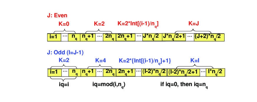
Figure 1: (Color online) Distributions of the $K$ quantum number (K) and $q$ values (iq) in the full $K\bigotimes q$ space. The dimension of the direct product of the $K$-subspace and the $q$-subspace is $D=(J+2)n_{q}/2$ for even $J$, or $D=(J-1)n_{q}/2$ for odd $J$. $n_{q}$ is the number of points on the mesh in $q$-space, and $J$ is the total angular momentum.

The domain of quadrupole deformation parameters $q\equiv(\beta,\gamma)$ is discretized, and the HWG integral equation is transformed into a matrix eigenvalue equation. The corresponding kernels $\mathscr{O}^{J}_{KK^{\prime}}(q,q^{\prime})$ have to be calculated between all pairs of mesh points in $q$ space. In the current version of the model the full space $K\bigotimes q$ is a direct product of the $K$-subspace and the $q$-subspace, with dimension $D=(J+2)n_{q}/2$ for even $J$ or $D=(J-1)n_{q}/2$ for odd $J$. $n_{q}$ is the number of points on the mesh in $q$-space, and $J$ the total angular momentum. Correspondingly, the kernels $\mathscr{O}^{J}_{KK^{\prime}}(q,q^{\prime})$ $\longrightarrow$ $\mathscr{O}^{J}(i,j)$. The quantum number $K$ and the value of $(\beta,\gamma)$ at each point of the full space $K\bigotimes q$ can be determined as shown in Fig. 1.

The first step in the solution of the HWG matrix eigenvalue equation is the diagonalization of the norm overlap kernel $\mathscr{N}^{J}(i,j)$

$$\sum_{j}\mathscr{N}^{J}(i,j)u^{J}_{k}(j)=n^{J}_{k}u^{J}_{k}(i).$$ (23)

Since the basis functions $|\Phi(q)\rangle$ are not linearly independent, many of the eigenvalues $n^{J}_{k}$ are very close to zero. They correspond to “high momentum” collective components, i.e., the corresponding eigenfunctions $u^{J}_{k}(i)$ are rapidly oscillating in the $q$-space but carry very little physical information. However, due to numerical uncertainties, their contribution to the matrix elements of the collective Hamiltonian (24) can be large, and these states should be removed from the basis. Therefore, a small positive constant $\zeta$ is introduced so that states with $n^{J}_{k}/n^{J}_{\textrm{m}ax}<\zeta$ are excluded from the GCM basis, where $n^{J}_{\textrm{m}ax}$ is the largest eigenvalue of the norm kernel. From the remaining states, also called “natural states”, one builds the collective Hamiltonian

$$\mathcal{H}^{J}_{kl}=\frac{1}{\sqrt{n^{J}_{k}}}\frac{1}{\sqrt{n^{J}_{l}}}\sum_{i,j}{u^{J}_{k}(i)\mathscr{H}^{J}(i,j)u^{J}_{l}(j)}\;,$$ (24)

which is subsequently diagonalized

$$\sum_{l}\mathcal{H}^{J}_{kl}g_{l}^{J\alpha}=E^{J}_{\alpha}g_{k}^{J\alpha}\;.$$ (25)

The solution of Eq. (25) determines both the energies $E^{J}_{\alpha}$ and the amplitudes $f^{JK}_{\alpha}(q)$ of collective states with good angular momentum $|\Psi^{JM}_{\alpha}\rangle$

$$f^{JK}_{\alpha}(q)=\sum\limits_{k}\frac{g_{k}^{J\alpha}}{\sqrt{n^{J}_{k}}}u^{J}_{k}(i).$$ (26)

The weight functions $f^{JK}_{\alpha}(q)$ are not orthogonal and cannot be interpreted as collective wave functions for the deformation variables. The collective wave functions $g^{J}_{\alpha}(i)$ are calculated from the norm overlap eigenstates:

$$g^{J}_{\alpha}(i)=\sum\limits_{k}g_{k}^{J\alpha}u^{J}_{k}(i),$$ (27)

$g^{J}_{\alpha}(i)$ are orthonormal and, therefore, $|g^{J}_{\alpha}(i)|^{2}$ can be interpreted as a probability amplitude.

The center-of-mass (c.m.) correction is defined by:

$$\langle E_{\mathrm{cm}}\rangle(J_{\alpha})=\langle\Psi^{JM}_{\alpha}|\dfrac{\hat{\mathbf{P}}_{\mathrm{cm}}^{2}}{2mA}|\Psi^{JM}_{\alpha}\rangle$$

$$= \sum_{ij}\sum_{KK^{\prime}}f^{JK\ast}_{\alpha}(i)f^{JK^{\prime}}_{\alpha}(j)\frac{1}{2mA}\langle\Phi(q_{i})|\hat{\mathbf{P}}_{\mathrm{cm}}^{2}P_{KK^{\prime}}^{J}|\Phi(q_{j})\rangle\;.$$

The projected overlap matrix elements $\langle\Phi(q_{i})|\hat{\mathbf{P}}_{\mathrm{cm}}^{2}P_{KK^{\prime}}^{J}|\Phi(q_{j})\rangle$ are treated in zeroth order of the Kamlah approximation, i.e. considering the fact that $\langle\Phi(q_{i})|\Phi(q_{j})\rangle$ is sharply peaked at $q_{i}=q_{j}$, the projected matrix elements are approximated by the unprojected ones Ring and Schuck (1980), and

$$\frac{1}{2mA}\langle\Phi(q_{i})|\hat{\mathbf{P}}_{\mathrm{cm}}^{2}\hat{P}_{KK^{\prime}}^{J}|\Phi(q_{j})\rangle\approx\mathscr{N}^{J}_{KK^{\prime}}(q_{i},q_{j})E_{\mathrm{cm}}(q_{i})\;,$$

were $E_{\mathrm{cm}}(q)$ is the c.m. correction evaluated for the intrinsic wave functions $|\Phi(q)\rangle$,

$$E_{\mathrm{cm}}(q)=\frac{1}{2mA}\langle\Phi(q)|\hat{\mathbf{P}}_{\mathrm{cm}}^{2}|\Phi(q)\rangle\;,$$ (30)

where $m$ is the nucleon mass, and $A$ is the number of nucleons. $\hat{\mathbf{P}}_{\rm cm}=\sum_{i}^{A}\hat{\mathbf{p}}_{i}$ is the total momentum. The energy of the collective state $|\Psi^{J}_{\alpha}\rangle$ is, therefore, given by

$$\mathbb{E}(J^{+}_{\alpha})=E^{J}_{\alpha}+\langle E_{\rm cm}\rangle(J_{\alpha})\;.$$ (31)

Once the amplitudes $f^{JK}_{\alpha}(q)$ of nuclear collective wave functions $|\Psi^{JM}_{\alpha}\rangle$ are known, it is straightforward to calculate all physical observables, such as the electromagnetic transition probability, spectroscopic quadrupole moments and the average particle number. The $B(E2)$ probability for a transition from an initial state $(J_{i},\alpha_{i})$ to a final state $(J_{f},\alpha_{f})$ is defined by

$$B(E2;J_{i},\alpha_{i}\rightarrow J_{f},\alpha_{f})$$ (32)

$$= \frac{e^{2}}{2J_{i}+1}\left|\sum_{q_{f},q_{i}}\langle J_{f},q_{f}||\hat{Q}_{2}||J_{i},q_{i}\rangle\right|^{2}\;,$$

Using the generalized Wigner-Eckart theorem for the spherical tensor operator $\hat{Q}_{\lambda\mu}$

$$\hat{P}^{J}_{KM}\hat{Q}_{\lambda\mu}\hat{P}^{J^{\prime}}_{M^{\prime}K^{\prime}}=C^{J\,M}_{J^{\prime}M^{\prime}\lambda\mu}\sum_{\bar{K}\mu^{\prime}}C^{J\,K}_{J^{\prime}\bar{K}\lambda\mu^{\prime}}\hat{Q}_{\lambda\mu^{\prime}}\hat{P}^{J^{\prime}}_{\bar{K}K^{\prime}}$$ (33)

and the relation

$$\hat{P}^{J}_{MK}\hat{P}^{J^{\prime}}_{M^{\prime}K^{\prime}}=\delta_{JJ^{\prime}}\delta_{KM^{\prime}}\hat{P}^{J}_{MK^{\prime}}$$ (34)

for projection operators Ring and Schuck (1980), one obtains for the reduced matrix element $\langle J_{f},q_{f}||\hat{Q}_{2}||J_{i},q_{i}\rangle$:

$$\langle J_{f},q_{f}||\hat{Q}_{2}||J_{i},q_{i}\rangle={\hat{J}}_{f}\sum_{K_{i}K_{f}}f^{\ast J_{f}K_{f}}_{\alpha_{f}}(q_{f})f^{J_{i}K_{i}}_{\alpha_{i}}(q_{i})~{}~{}~{}~{}~{}$$ (35)

$$\times\sum_{\mu K^{\prime}}(-1)^{J_{f}-K_{f}}\left(\begin{array}[]{ccc}J_{f}&2&J_{i}\\ -K_{f}&\mu&K^{\prime}\\ \end{array}\right)Q_{2\mu}(K^{\prime},K_{i};q_{f},q_{i})$$ (38)

with ${\hat{J}}_{f}=2J_{f}+1$, $f^{JK}_{\alpha}(q)=(-1)^{J}f^{J-K}_{\alpha}(q)$ for $K<0$, and

$$Q_{2\mu}(K^{\prime},K_{i};q_{f},q_{i})\equiv\langle\Phi(q_{f})|\hat{Q}_{2\mu}\hat{P}^{J_{i}}_{K^{\prime}K_{i}}|\Phi(q_{i})\rangle.$$ (39)

More details on the calculation of the reduced $E2$ matrix element are given in Appendix A. The matrix elements of the charge quadrupole operator $\hat{Q}_{2\mu}=e\sum_{p}r^{2}_{p}Y_{2\mu}(\Omega_{p})$ are calculated in the full configuration space. There is no need for effective charges, and $e$ simply corresponds to the bare value of the proton charge.

Electric monopole (E0) transitions are calculated from the off-diagonal matrix elements of the $E0$ operator. The corresponding diagonal matrix elements are directly related to mean-square charge radii that provide signatures of shape changes in nuclei. The relation between E0 transitions and shape transitions and coexistence phenomena has been extensively investigated Wood et al. (1992, 1999); Zerguine et al. (2008); Wiedeking et al. (2008). The $E0$ transition rate $\tau(E0)$ between $0^{+}_{1}$ and $0^{+}_{2}$ can be separated into two factors: the electronic and the nuclear Wood et al. (1999)

$$\dfrac{1}{\tau(E0)}=\rho^{2}_{21}\Omega\;,$$ (40)

where the nuclear factor $\rho^{2}_{21}$ is defined by:

$$\rho^{2}_{21}(E0)=\left|\langle 0^{+}_{2}|\hat{T}(E0)|0^{+}_{1}\rangle\right|^{2}/e^{2}R^{4}_{0},$$ (41)

and $\hat{T}(E0)=\sum_{k}e_{k}r^{2}_{k}$. The off-diagonal matrix elements of the $E0$ operator can be evaluated using angular momentum projected GCM wave functions:

$$\langle 0^{+}_{2}|\hat{T}(E0)|0^{+}_{1}\rangle$$ (42)

$$= \sum_{q_{i},q_{j}}f^{\ast}_{0^{+}_{2}}(q_{j})f_{0^{+}_{1}}(q_{i})\langle\Phi(q_{j})|\hat{T}(E0)\hat{P}^{0}_{00}|\Phi(q_{i})\rangle\;.$$

Finally, it will be useful to check the average number of particles for a collective state $|\Psi^{JM}_{\alpha}\rangle$:

$$N^{J}_{\alpha} = \langle\Psi^{JM}_{\alpha}|\hat{N}|\Psi^{JM}_{\alpha}\rangle$$ (43)

$$= \sum_{q_{j},q_{i};K_{1},K_{2}}\Delta_{K_{1}K_{2}}f^{\ast JK_{2}}_{\alpha}(q_{j})f^{JK_{1}}_{\alpha}(q_{i})$$

$$\times\int d\Omega D^{J\ast}_{K_{2}K_{1}}\langle\Phi(q_{j})|\hat{N}\hat{R}(\Omega)|\Phi(q_{i})\rangle\;,$$

where $\hat{N}=\sum_{k}a^{\dagger}_{k}a_{k}$ is the particle number operator, and

$$\dfrac{\langle\Phi(q_{j})|\hat{N}\hat{R}(\Omega)|\Phi(q_{i})\rangle}{\langle\Phi(q_{j})|\hat{R}(\Omega)|\Phi(q_{i})\rangle}=\int d\bm{r}\rho_{V}(\bm{r};q_{j},q_{i};\Omega)\;.$$ (44)

$\rho_{V}(\bm{r})$ is the zeroth component of the nucleon vector current (cf. Eq. 11c), and the expression for the corresponding transition vector density $\rho_{V}(\bm{r};q_{j},q_{i};\Omega)$ has been given in Ref. Yao et al. (2009). Since the intrinsic state $|\Phi(q_{i})\rangle$ corresponds to a BCS wave function, i.e. it is not an eigenstate of the particle number operator, the trace of the transition density in Eq.(44) generally does not equal the total nucleon number.

III The low-spin spectrum of ²⁴Mg

In this section we perform several illustrative configuration mixing calculations that will test our implementation of the 3D angular momentum projection and the generator coordinate method. The intrinsic wave functions that are used in the configuration mixing calculation have been obtained as solutions of the self-consistent relativistic mean-field equations, subject to constraint on the axial and triaxial mass quadrupole moments. The interaction in the particle-hole channel is determined by the relativistic density functional PC-F1 Burvenich et al. (2002), and a density-independent $\delta$-force is used as the effective interaction in the particle-particle channel. Pairing correlations are treated in the BCS approximation. The pairing strength parameters $V_{\tau}$ ($\tau=p,n$) are adjusted by fitting the average gaps of the mean-field ground state Dobaczewski et al. (1984) of ²⁴Mg

$$\langle\Delta\rangle\equiv\frac{\sum_{k}f_{k}v_{k}^{2}\Delta_{k}}{\sum_{k}f_{k}v_{k}^{2}}\;,$$ (45)

to the experimental values obtained from odd-even mass differences using the five-point formula: $\Delta^{(5)}_{\rm n}=3.193$ MeV, and $\Delta^{(5)}_{\rm p}=3.123$ MeV. The quantities $f_{k}$ are defined in Eq.(14) and $v^{2}_{k}$ are the occupation probabilities of single-nucleon states. The resulting pairing strengths are $V_{n}=511.300$ fm³ MeV for neutrons, and $V_{p}=518.350$ fm³ MeV for protons. We note that these values differ from the universal parameters of Ref. Burvenich et al. (2002), that have been adjusted to pairing properties of heavy nuclei. With the original pairing strengths of Ref. Burvenich et al. (2002), the resulting gaps for ²⁴Mg are considerably smaller than the ones obtained from experimental odd-even mass differences.

Parity, $D_{2}$-symmetry, and time-reversal invariance are imposed in the mean-field calculation, and this implies that the space-like components of the single-nucleon four-currents ($j^{\mu},j^{\mu}_{TV}$) vanish. The scalar ($\rho_{S},\rho_{TS}$) and vector ($\rho_{V},\rho_{TV}$) densities in the EDF of Eq. (II) are symmetric under reflections with respect to the $yz$, $xz$ and $xy$ planes. Obviously these symmetries are not fulfilled by the transition densities and, therefore, the octant $x,y,z\geq 0$ must be extended to the entire coordinate space when evaluating transition densities.

To solve the Dirac equation for triaxially deformed potentials, the single-nucleon spinors are expanded in the basis of eigenfunctions of a three-dimensional harmonic oscillator (HO) in Cartesian coordinate Koepf and Ring (1988) with $N_{\mathrm{sh}}$ major shells. In Ref. Yao et al. (2009) it has been shown that $N_{\mathrm{sh}}=8$ is sufficient to obtain a reasonably converged mean-field potential energy curve for ²⁴Mg. The HO basis is chosen isotropic, i.e. the oscillator parameters $b_{x}=b_{y}=b_{z}=b_{0}=\sqrt{\hbar/m\omega_{0}}$ in order to keep the basis closed under rotations Egido et al. (1993); Robledo (1994). The oscillator frequency is given by $\hbar\omega_{0}=41A^{-1/3}$. The Gaussian-Legendre quadrature is used for integrals over the Euler angles $\phi,\theta$ and $\psi$ in the calculation of the norm and hamiltonian kernels. With the choice of the number of mesh points for the Euler angles in the interval $[0,\pi]$: $N_{\phi}=N_{\psi}=8$, and $N_{\theta}=12$, the calculation achieves an accuracy of $\approx 0.05\%$ for the energy of a projected state with angular momentum $J\leq 6$ in the ground-state band Yao et al. (2009).

The nucleus ²⁴Mg presents an illustrative test case for the 3DAMP+GCM approach to low-energy nuclear structure. The principal motivation for considering this nucleus is the direct comparison of the present analysis with the results of Ref. Bender and Heenen (2008), where a 3DAMP+GCM model has been developed based on Skyrme triaxial mean-field states that are projected on particle number and angular momentum, and mixed by the generator coordinate method. Collective phenomena are, of course, much more pronounced in heavy nuclei and, therefore, the goal is to eventually apply the present approach to the rare earth nuclides and the Actinide region. This will require not only a large oscillator basis, but also a large number of mesh-points for the Gaussian quadrature in coordinate space, as well as a finer mesh for the Euler angles and the deformation parameters.

Axially symmetric AMP+GCM calculations are at present routinely performed for heavy nuclei Nikšić et al. (2006a), and from such studies one can estimate that $N_{f}\approx 16$ shells have to be included in the oscillator basis for the systems in the mass region around Pb. Note that the computing time necessary for the evaluation of one overlap matrix element scales approximately with $N_{f}^{6}$. For instance, the number of mesh-points in the axial deformation $\beta$ that was used in Ref. Nikšić et al. (2006a) is a factor 4 larger than in the present analysis and, moreover, in the 3D case one also needs a finer mesh for the integration over Euler angles. These considerations show that a straightforward application of the existing 3DAMP+GCM codes to $A\approx 200$ heavy nuclei will basically depend on the availability of large-scale general-purpose computer resources. On the other hand, the introduction of additional approximations could considerably reduce the computing requirements. For instance, the overlap functions are strongly peaked at $q=q^{\prime}$, and the use of Gaussian overlap approximations has produced excellent results in many cases. These approximations form the basis for the derivation of a collective Bohr Hamiltonian for quadrupole degrees of freedom Nikšić et al. (2009); Li et al. (2009).

III.1 Convergence of the 3DAMP+GCM calculations

The convergence of the 3DAMP+GCM calculation has been examined with respect to both the number of mesh points in the ($\beta,\gamma$) plane, and the cutoff parameter $\zeta$ that is used to remove from the GCM basis the eigenstates of the norm overlap kernel $\mathscr{N}^{J}$ with very small eigenvalues $n^{J}_{k}/n^{J}_{\textrm{m}ax}<\zeta$. In the first step the cutoff is set to $\zeta=5\times 10^{-3}$, and we compare low-lying spectra of ²⁴Mg that are obtained in 3DAMP+GCM calculations with different numbers of points of the discretized generator coordinates. We consider the following sets of generator coordinates: (AI, AII, AIII) include only axial deformations (prolate and oblate shapes)

• AI: $(\beta,\gamma)=(0.1,0^{\circ})$, (0.3, 0^∘), (0.5, 0^∘), (0.7, 0^∘), (0.9, 0^∘), (1.1, 0^∘);

• AII: $(\beta,\gamma)=(0.1,0^{\circ}$), (0.1, 60^∘), (0.3, 0^∘), (0.3, 60^∘), (0.5, 0^∘), (0.5, 60^∘), (0.7, 0^∘), (0.7, 60^∘), (0.9, 0^∘), (0.9, 60^∘), (1.1, 0^∘), (1.1, 60^∘);

• AIII: $(\beta,\gamma)=(0,0^{\circ}$), (0.1, 0^∘), (0.1, 60^∘), (0.2, 0^∘), (0.2, 60^∘), (0.3, 0^∘), (0.3, 60^∘), (0.4, 0^∘), (0.4, 60^∘), (0.5, 0^∘), (0.5, 60^∘), (0.6, 0^∘), (0.6, 60^∘), (0.7, 0^∘), (0.7, 60^∘), (0.8, 0^∘), (0.8, 60^∘), (0.9, 0^∘), (0.9, 60^∘), (1.0, 0^∘), (1.0, 60^∘), (1.1, 0^∘), (1.1, 60^∘)  .

(TI, TII, TIII) denote different sets with $\gamma\neq 0$ (triaxial shapes):

• TI: $\gamma=0^{\circ},30^{\circ},60^{\circ}$;

• TII: $\gamma=0^{\circ},20^{\circ},40^{\circ},60^{\circ}$;

• TIII: $\gamma=0^{\circ},10^{\circ},20^{\circ},30^{\circ},40^{\circ},50^{\circ},60^{\circ}$.

The sets of ($\beta,\gamma$) mesh-points shown in Fig. 2 have been used in the present analysis.

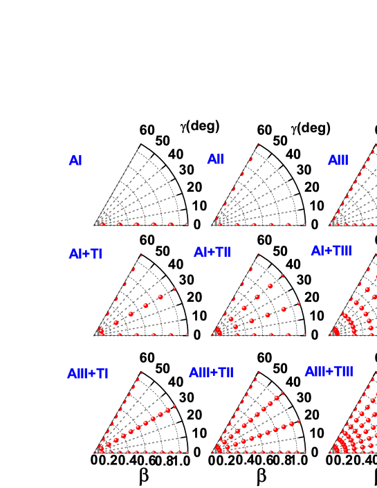
Figure 2: (Color online) The distribution of mesh points in the ($\beta,\gamma$) plane for the sets AI, AII, AIII, AI+TI, AI+TII, AI+TIII, AIII+TI, AIII+TII and AIII+TIII.

Table 1: Ground state energies $E_{gs}$, excitation energies $E_{x}$ (in MeV) and $B(E2)$ values (in e²fm⁴) for transitions between low-spin states in ²⁴Mg, calculated with the 3DAMP+GCM model for the generator coordinate sets AI, AII and AIII (see text for details).

quantities	AI	AII	AIII
$E_{gs}$($0^{+}_{1}$)	-196.985	-197.291	-197.279
$E_{x}$($2^{+}_{1}$)	2.196	2.351	2.330
$E_{x}$($4^{+}_{1}$)	5.394	5.905	5.849
$E_{x}$($6^{+}_{1}$)	10.426	10.591	10.568
$B(E2:2^{+}_{1}\rightarrow 0^{+}_{1}$)	78.155	78.721	79.135
$B(E2:4^{+}_{1}\rightarrow 2^{+}_{1}$)	137.679	140.814	139.750
$B(E2:6^{+}_{1}\rightarrow 4^{+}_{1}$)	177.025	169.246	168.527

Table 2: Same as Table 1, but for the generator coordinates sets AI+TI, AI+TII and AI+TIII (see text for details).

quantities	AI+TI	AI+TII	AI+TIII
$E_{gs}$($0^{+}_{1}$)	-197.285	-197.304	-197.307
$E_{x}$($2^{+}_{1}$)	2.241	2.198	2.177
$E_{x}$($4^{+}_{1}$)	5.776	5.725	5.677
$E_{x}$($6^{+}_{1}$)	10.485	10.413	10.360
$B(E2:2^{+}_{1}\rightarrow 0^{+}_{1}$)	80.523	80.849	81.435
$B(E2:4^{+}_{1}\rightarrow 2^{+}_{1}$)	144.441	145.926	147.178
$B(E2:6^{+}_{1}\rightarrow 4^{+}_{1}$)	171.275	178.015	182.199

In Table 1 we display the excitation energies and $B(E2)$ values of low-spin yrast states in ²⁴Mg, calculated with the 3DAMP+GCM model, but including only axially deformed mean-field states (coordinate sets AI, AII and AIII, as shown in Fig. 2). One notes that the largest differences in the calculated excitation energies are within 10 % and the $B(E2:J\rightarrow J-2)$ values agree within 5 %. The major step for the energies comes from the inclusion of oblate shapes (AII) in the GCM configuration mixing calculations. It lowers the total ground state energy by $\approx 300$ keV and increases the energies by $\approx 150$ keV for the $2^{+}_{1}$, 200 keV for the $4^{+}_{1}$, and 150 keV for the $6^{+}_{1}$ state. The refinement of the mesh in AIII produces only small changes.

Similar results are found when comparing results of 3DAMP+GCM calculations based on triaxial intrinsic states: AI+TI, AI+TII and AI+TIII in Table II, and AIII+TI, AIII+TII and AIII+TIII in Table III. The effect of including triaxial deformations, i.e. the $\gamma$ degree of freedom, is perhaps best illustrated in the comparison between results obtained with the sets of generator coordinates AIII (Tab. 1) and AIII+TIII (Tab. 3). The inclusion of triaxial states in the GCM configuration mixing calculation lowers the total energies by 39 keV for $0^{+}_{1}$, 180 keV for $2^{+}_{1}$, 226 keV for $4^{+}_{1}$, and 262 keV for $6^{+}_{1}$. The corresponding $B(E2:J\rightarrow J-2)$ values are enhanced by $3.94\%,5.29\%,7.63\%$ for $J^{\pi}_{\alpha}=2^{+}_{1},4^{+}_{1},6^{+}_{1}$, respectively.

The influence of the $\gamma$ degree of freedom, and the convergence of 3DAMP+GCM calculations with respect to the number of mesh points of the discretized generator coordinates can clearly be seen in the comparison of calculations with mean-field states at the mesh points of coordinate sets AI, AI+TIII and AIII, AIII+TIII. The inclusion of triaxial shapes lowers the energies by $\approx 300$ keV. On the other hand, very similar results are obtained in calculations based on coordinate sets that differ only in the number of axial points. Therefore, we find that, if prolate as well as oblate configurations are included, the spectroscopic properties of low-spin states in ²⁴Mg are not very sensitive to the number of axial meshpoints. The inclusion of the $\gamma$ degree of freedom changes this situation somewhat, but not dramatically for the ground stated band where the admixtures with $K\neq 0$ are small. This is consistent with the results of the 3DAMP+GCM calculation with particle-number projection Bender and Heenen (2008), based on the non-relativistic Skyrme density functional. It was shown, namely, that the number of axial states that can be added to the set of triaxial states is not large. Redundancies appear very quickly in the norm kernel when more states are added to the nonorthogonal basis, and this is simply a consequence of very few level crossings as function of deformation in ²⁴Mg.

Table 3: Same as Table 1, but for the generator coordinates sets AIII+TI, AIII+TII and AIII+TIII (see text for details).

quantities	AIII+TI	AIII+TII	AIII+TIII
$E_{gs}$($0^{+}_{1}$)	-197.290	-197.306	-197.318
$E_{x}$($2^{+}_{1}$)	2.239	2.205	2.189
$E_{x}$($4^{+}_{1}$)	5.735	5.695	5.662
$E_{x}$($6^{+}_{1}$)	10.452	10.388	10.345
$B(E2:2^{+}_{1}\rightarrow 0^{+}_{1}$)	80.498	81.488	82.256
$B(E2:4^{+}_{1}\rightarrow 2^{+}_{1}$)	143.042	145.525	147.137
$B(E2:6^{+}_{1}\rightarrow 4^{+}_{1}$)	166.952	175.157	181.379

In Table 4 we show the excitation energies and $B(E2)$ values for low-lying states in ²⁴Mg, calculated with the 3DAMP+GCM model based on a set of axial mean-field states with $\beta=0,0.1,0.2,\cdots,1.1$ and $\gamma=0^{\circ},60^{\circ}$, as functions of the cutoff parameter $\zeta$, that defines the basis of “natural states”. Eigenstates of the norm overlap kernel $\mathscr{N}^{J}$ with eigenvalues $n^{J}_{k}/n^{J}_{\textrm{m}ax}<\zeta$ are removed from the GCM basis ($n^{J}_{\textrm{m}ax}$ is the largest eigenvalue of the norm kernel for a given angular momentum). The excitation energies are not sensitive to the particular value of the cutoff parameter provided $\zeta<1\times 10^{-2}$, whereas the effect on the $B(E2)$ values is $<1\%$ for smaller values of $\zeta$. However, $\zeta$ cannot be taken arbitrarily small, because spurious states are introduced in the basis for very small eigenvalues of the norm overlap kernel. The remaining calculations presented in this work have been performed using the value $\zeta=5\times 10^{-3}$.

Table 4: Excitation energies $E_{x}$ (in MeV) and $B(E2)$ values (in e²fm⁴) for transitions between low-spin states in ²⁴Mg, calculated with the 3DAMP+GCM model for the generator coordinates $\beta=0,0.1,\cdots,1.1$, and $\gamma=0^{\circ},60^{\circ}$ as functions of the cutoff parameter $\zeta$ that defines the basis of “natural states”.

$\zeta$	$5\times 10^{-2}$	$1\times 10^{-2}$	$5\times 10^{-3}$	$1\times 10^{-3}$	$5\times 10^{-4}$	$1\times 10^{-4}$
$E_{x}$($2^{+}_{1}$)	2.275	2.340	2.330	2.341	2.314	2.320
$E_{x}$($4^{+}_{1}$)	5.703	5.931	5.849	5.573	5.544	5.580
$B(E2:2^{+}_{1}\rightarrow 0^{+}_{1}$)	77.586	80.138	79.135	79.967	79.113	79.688
$B(E2:4^{+}_{1}\rightarrow 2^{+}_{1}$)	144.403	143.314	139.750	136.372	137.989	138.669

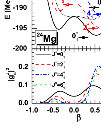
Figure 3: (Color online) Upper panel: energies and the average axial deformations for the two lowest GCM states with angular momentum $0^{+},2^{+},4^{+},6^{+}$ in ²⁴Mg, together with the mean-field (dotted) and the corresponding angular-momentum projected energy curves. Lower panel: squares of collective wave functions $|g^{J}_{\alpha}(q)|^{2}$ with $q_{22}=0$ for the corresponding lowest GCM states in ²⁴Mg. These results are obtained in the axial 1DAMP+GCM calculation. Positive (negative) values of the axial deformation $\beta$ correspond to prolate (oblate) configurations.

III.2 Axially-symmetric AMP+GCM calculation

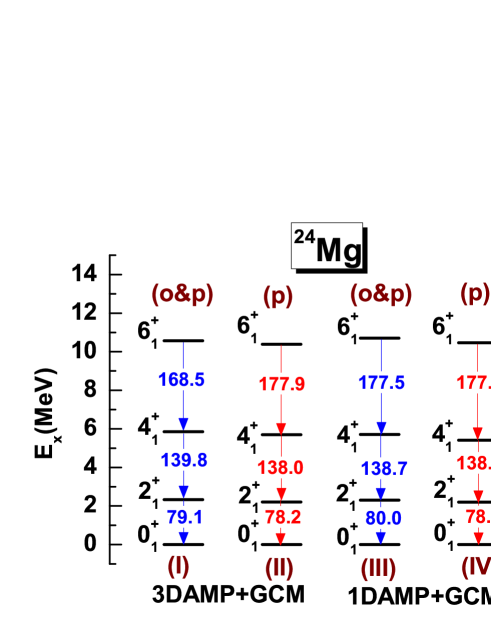
Figure 4: (Color online) Lowest energy levels of angular momentum $J^{\pi}=0^{+}$, $2^{+}$, $4^{+}$, $6^{+}$ in ²⁴Mg, and reduced $E2$ transition probabilities in e²fm⁴, calculated with the 3DAMP+GCM and 1DAMP+GCM models. See text for details.

By restricting the set of intrinsic states to axially symmetric configurations: $\gamma=0$ and $\gamma=180^{\circ}$, the complicated 3DAMP+GCM model is reduced to a relatively simple 1DAMP+GCM calculation. For the choice of generator coordinates $\beta=0,0.1,0.2,\cdots,1.1$; $\gamma=0$ and $\gamma=180^{\circ}$, we have calculated the energies and the average axial quadrupole deformations of the two lowest GCM states, for each angular momentum: $0^{+}$, $2^{+}$, $4^{+}$, and $6^{+}$ in ²⁴Mg, as shown in Fig. 3.

The mean-field energy surface is somewhat soft with a prolate deformed minimum at $\beta\approx 0.50,\gamma=0^{\circ}$, and the total energy $E=-192.807$ MeV. This result is consistent with our previous calculation that used the PC-F1 energy density functional plus a monopole pairing force Yao et al. (2008), and with an earlier study that employed the relativistic mean-field model with the NL2 effective interaction Koepf and Ring (1988). A rotational yrast band is calculated in the prolate minimum, with the squares of collective wave functions (probabilities) concentrated at $\beta\approx 0.5$.

In Fig. 4 we display the lowest energy levels of angular momentum $J^{\pi}=0^{+}$, $2^{+}$, $4^{+}$, $6^{+}$ in ²⁴Mg, calculated with the 3DAMP+GCM and 1DAMP+GCM codes, for the sets of axially symmetric generator coordinates: $\beta=0,0.1,0.2,\cdots,1.1$ with both prolate ($\gamma=0$) and oblate states ($\gamma=60^{\circ}$ and $\gamma=180^{\circ}$ in 3DAMP+GCM and 1DAMP+GCM models, respectively) (columns I and III), and with only prolate states $\gamma=0$ (columns II and IV). As expected, the 3DAMP+GCM and 1DAMP+GCM calculations produce virtually identical results, with small differences attributed to the numerical accuracy. In fact, the difference between the $B(E2)$ values shown in columns I and III can be further reduced by increasing the number of mesh-points used in the Gaussian-Legendre quadrature over the Euler angles $\phi,\theta$ and $\psi$ in the calculation of the norm and hamiltonian kernels.

III.3 Triaxial AMP+GCM calculation

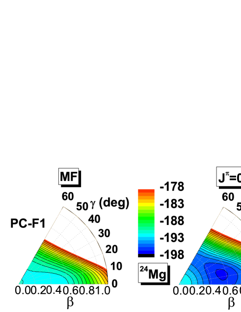
Figure 5: (Color online) Self-consistent RMF+BCS energy surface (left panel) of ²⁴Mg in the $\beta$-$\gamma$ plane ($0\leq\gamma\leq 60^{0}$), and angular momentum projected energy surface with $J^{\pi}=0^{+}$ (right panel). The contours join points on the surface with the same energy. The difference between neighboring contours is 1.0 MeV.

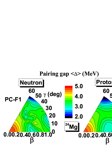
Figure 6: (Color online) Average neutron and proton pairing gaps of ²⁴Mg in the $\beta$-$\gamma$ plane ($0\leq\gamma\leq 60^{0}$). The contours join points on the surface with the same pairing gap. The difference between neighboring contours is 0.2 MeV.

Figure 7: (Color online) The low-spin level scheme of ²⁴Mg calculated using the 3DAMP+GCM model and 1DAMP+GCM model with the PC-F1 relativistic density functional, in comparison with data Endt (1993); Branford et al. (1975); Keinonen et al. (1989). The $B(E2)$ values are given in units of e²fm⁴.

In Fig. 5 we plot the self-consistent RMF+BCS triaxial energy surface of ²⁴Mg in the $\beta$-$\gamma$ plane ($0\leq\gamma\leq 60^{0}$), obtained by imposing constraints on the expectation values of the quadrupole moments $q_{20}$ and ${q}_{22}$. The panel on the right displays the projected energy surface with $J^{\pi}=0^{+}$:

$$E^{J=0}(q)={{\mathscr{H}^{J=0}(q,q)}\over{\mathscr{N}^{J=0}(q,q)}}$$ (46)

The contours join points with the same energy and the difference between neighboring contours is 1.0 MeV. The energy surfaces nicely illustrate the effects of including triaxial shapes and of the restoration of rotational symmetry. The mean-field energy surfaces are found to be quite soft with a minimum at an axial prolate deformation $\beta\approx 0.5$. When compared with the axial plot in Fig. 3, one realizes that the oblate minimum on the axial projected energy curve with $J^{\pi}=0^{+}$ is actually a saddle point in $\gamma$ direction. Projection shifts the minimum to a slightly triaxial shape with $\beta=0.50,\gamma=20^{\circ}$ and $E=-197.074$ MeV. The gain in energy from the restoration of rotational symmetry is $4.266$ MeV. The fact that angular momentum projection leads to triaxial minima in the PES was already noted in 3DAMP calculations in the eighties Hayashi et al. (1984), and very similar results have been obtained recently Bender and Heenen (2008) for the nucleus ²⁴Mg using the Skyrme functional SLy4. We note, however, that the 3DAMP+GCM model used in Ref. Bender and Heenen (2008) includes a projection on proton and neutron numbers, that is not carried out in the present analysis.

Fig. 6 displays the corresponding average neutron and proton pairing gaps $\langle\Delta\rangle$, defined by Eq. (45), as functions of deformation variables $\beta$ and $\gamma$. The gaps are relatively small around the minimum of the potential energy surface (PES), whereas larger values are calculated at the saddle points. The fluctuations of pairing gaps reflect the underlying shell structure.

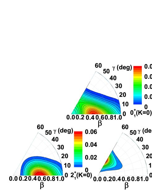
Figure 8: (Color online) Contour plots of the probability distributions $|g^{J}_{\alpha}|^{2}$ for the ground state $0^{+}_{1}$ and the first excited state $2^{+}_{1}$ (both the $K=0$ and $K=2$ components) in ²⁴Mg.

The solution of the HWG equation (16) yields the excitation energies and the collective wave functions for each value of the total angular momentum and parity $J^{\pi}$. In addition to the yrast ground-state band, in deformed and transitional nuclei excited states are usually also assigned to (quasi) $\beta$ and $\gamma$ bands. This is done according to the distribution of the angular momentum projection $K$ quantum number (Figs. 8-10). Excited states with predominant $K=2$ components in the wave function are assigned to the $\gamma$-band, whereas the $\beta$-band comprises states above the yrast characterized by dominant $K=0$ components. As an example, in Fig. 7 we display the low-spin PC-F1 excitation spectrum of ²⁴Mg obtained by the 1DAMP+GCM calculation with the AIII set of generator coordinates, and by the 3DAMP+GCM calculation with the AIII+TIII set of mesh points, in comparison with available data Endt (1993); Branford et al. (1975); Keinonen et al. (1989). The level scheme is in rather good agreement with data, but in both cases the calculated spectra are systematically stretched as compared to experimental bands. This is because angular-momentum projection is performed only after variation and, therefore, time-odd components and alignment effects are neglected. Cranking calculations, for instance, correspond to an approximate angular-momentum projection before variation Beck et al. (1970), and lead to an enhancement of the moments of inertia in better agreement with data Koepf and Ring (1989); Afanasjev et al. (2000). However, at present the full 3D angular-momentum projection before variation, plus GCM configuration mixing, is still beyond the available computing capacities. The agreement of the calculated quadrupole transition probabilities with data in Fig. 7 is remarkable, especially considering that the calculation of B(E2) values is parameter-free, i.e. the transitions are calculated employing bare proton charges.

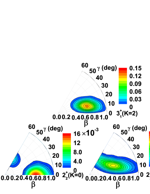
Figure 9: (Color online) Same as in Fig. 8, but for the excited states $3^{+}_{1}$ and $2^{+}_{2}$ in ²⁴Mg.

Figure 10: (Color online) Same as in Fig. 8, but for the excited states $4^{+}_{1}$ and $4^{+}_{2}$ in ²⁴Mg.

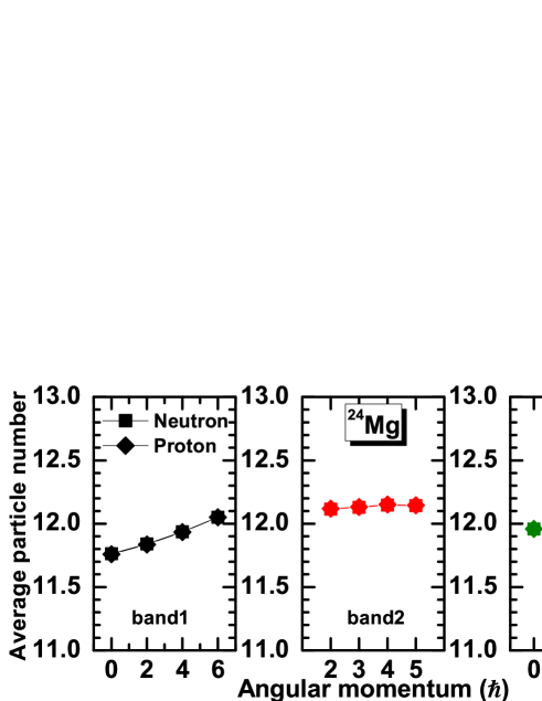
Figure 11: (Color online) Average particle numbers for the 3DAMP+GCM states belonging to the three bands of ²⁴Mg in Fig. 7.

In Fig. 8, we plot the corresponding distributions $|g^{J}_{\alpha}|^{2}$ of Eq. (27), with respect to $\beta$ and $\gamma$, for the ground state $0^{+}_{1}$ and the first excited state $2^{+}_{1}$ (both the $K=0$ and $K=2$ components) in ²⁴Mg. These quantities give the probabilities that the intrinsic wave functions of the corresponding states have a certain quadrupole deformation characterized by the collective coordinates $\beta$ and $\gamma$. For the ground state, and for the $K=0$ component of $2^{+}_{1}$, these distributions are largely concentrated along the prolate symmetry axis. Since the $K=0$ component of the $2^{+}_{1}$ state exhausts $92\%$ of the norm, this state obviously belongs to the $K=0$ band built on the nearly prolate ground state. From the PES shown in the right panel of Fig. 5, with the pronounced minimum at $\gamma\approx 20^{0}$, one would have expected the maximum of the probability distributions in this region of the ($\beta,\gamma$) plane. However, it turns out that the inclusion of quadrupole fluctuations through GCM configuration mixing, drives the structure built on the ground state back toward the prolate symmetry axis, i.e. the GCM model calculation does not predict the existence of a stable triaxial structure of the intrinsic states of the ground-state band of ²⁴Mg. The probability distributions for the excited states $3^{+}_{1}$ and $2^{+}_{2}$ are shown in Fig. 9. For $2^{+}_{2}$ state the $K=2$ component exhausts about $87\%$ of the norm and, therefore, $2^{+}_{2}$ and $3^{+}_{1}$ are assigned to the $K=2$ (quasi) $\gamma$ band. The $K=0$, $K=2$ and $K=4$ probability distributions of the states $4^{+}_{1}$ and $4^{+}_{2}$ are displayed in Fig. 10. Since the $K=0$ ($K=2$) component of the state $4^{+}_{1}$ ($4^{+}_{2}$) exhausts $92\%$ ($79\%$) of the norm, $4^{+}_{1}$ belongs to the ground-state band, and $4^{+}_{2}$ to the (quasi) $\gamma$ band.

Finally in Fig. 11 we display the average neutron and proton numbers (cf. Eq. (43)) for the 3DAMP+GCM states belonging to the three bands of ²⁴Mg in Fig. 7. The dispersion of the particle number is relative large $(\approx 0.3)$ for states $0^{+}_{1}$ and $2^{+}_{1}$.

IV Summary and Outlook

The framework of relativistic energy density functionals has been very successfully applied to the description of a rich variety of structure phenomena over the whole nuclear chart. However, to go beyond the modeling of bulk nuclear properties and perform detailed calculations of excitation spectra and transition probabilities, one must extend the simple single-reference (mean-field) implementation of this framework, and include long-range correlations related to restoration of symmetries broken by the static mean field and to fluctuations of collective coordinates around the mean-field minimum. Building on recent models Nikšić et al. (2006a, b) that have employed the generator coordinate method (GCM) to perform configuration mixing of axially-symmetric relativistic mean-field wave functions, and especially on Ref. Yao et al. (2009), where we have already considered three-dimensional angular-momentum projection (3DAMP) of relativistic mean-field wave functions, in this work a model has been developed that uses the GCM in configuration mixing calculations that involve 3DAMP wave functions, generated by constrained self-consistent mean-field calculations for triaxial nuclear shapes.

The current implementation of the relativistic 3DAMP+GCM model has been tested in the calculation of spectroscopic properties of low-spin states in ²⁴Mg. Starting with the relativistic density functional PC-F1 Burvenich et al. (2002), and a density-independent $\delta$-force as the effective interaction in the pairing channel, the intrinsic wave functions are generated from the self-consistent solutions of the constrained RMF+BCS equations in the basis of a three-dimensional harmonic oscillator in Cartesian coordinates. The constraints are on the axial and triaxial mass quadrupole moments. After restoring rotational symmetry by 3DAMP, the fluctuations of quadrupole deformations are included by performing GCM mixing of angular-momentum projected configurations that correspond to different values of the generator coordinates $\beta$ and $\gamma$. The GCM calculation has been tested both with respect to the number of mesh-points in the discretized ($\beta,\gamma$) plane, and the cutoff-parameter that is used to eliminate from the GCM basis the “high momentum” eigenvectors of the norm overlap kernels with extremely small eigenvalues. Results for excitation energies in the ground-state, (quasi) $\gamma$ and $\beta$ bands, and the corresponding interband and intraband transition probabilities have been compared with available data on low-spin states in ²⁴Mg. The comparison has shown a very good agreement between data and the predictions of the relativistic 3DAMP+GCM model.

The choice of ²⁴Mg allows a direct comparison of the present analysis with the results of Ref. Bender and Heenen (2008), where a 3DAMP+GCM model has been developed based on Skyrme triaxial mean-field states that are projected on particle number and angular momentum, and mixed by the generator coordinate method. Because it includes projection on particle number, the model of Ref. Bender and Heenen (2008) is much more involved and the numerical implementation is more difficult. In particular, the use of general EDFs in GCM calculations, i.e. energy functionals with an arbitrary dependence on nucleon densities, leads to discontinuities or even divergences of the energy kernels as functions of deformation, that can possibly produce spurious contaminations in the calculated excitation spectra (for a detailed discussion, we refer the reader to Refs. Anguiano et al. (2001); Bender et al. (2009); Lacroix et al. (2009), and references cited therein). Even though the results of the present calculation for ²⁴Mg are in good agreement with those of Ref. Bender and Heenen (2008), an important advantage of performing particle-number projection is that it prevents a collapse of pairing when the level density around the Fermi energy is reduced as, for instance, close to the minimum of the potential energy surface. The comparison with Ref. Bender and Heenen (2008) thus points to an obvious improvement of our 3DAMP+GCM model, i.e. the implementation of particle-number projection.

As an alternative approach to five-dimensional quadrupole dynamics that includes rotational symmetry restoration and takes into account triaxial quadrupole fluctuations, one can construct a collective Bohr Hamiltonian with deformation-dependent parameters. In a recent work Nikšić et al. (2009), we have developed a new implementation for the solution of the eigenvalue problem of a five-dimensional collective Hamiltonian for quadrupole vibrational and rotational degrees of freedom, with parameters determined by constrained self-consistent relativistic mean-field calculations for triaxial shapes. As in the present work, in addition to the self-consistent mean-field potential of the PC-F1 relativistic density functional in the particle-hole channel, for open-shell nuclei pairing correlations are included in the BCS approximation. In Ref. Li et al. (2009), the model has been applied in the study of shape phase transitions in the region $Z=60$, $62$, $64$ with $N\approx 90$. The collective Hamiltonian can be derived in the Gaussian overlap approximation (GOA) Ring and Schuck (1980) to the full five-dimensional GCM. With the assumption that the GCM overlap kernels can be approximated by Gaussian functions, the local expansion of the kernels up to second order in the non-locality transforms the HWG equation into a second-order differential equation for the collective Hamiltonian. Therefore, having developed both the five-dimensional quadrupole collective Hamiltonian, and the full 3DAMP+GCM model, we plan to perform microscopic tests of the GOA in a study of low-spin spectroscopy of $\gamma$-soft transitional nuclei, especially the effect of GOA on the calculated transitions between bands. In general, we expect that both models will be a useful addition to the theoretical tools that can be used in studies of complex structure phenomena in medium-heavy and heavy nuclei, including exotic systems far from stability.

Appendix A Reduced matrix element of the quadrupole operator

The basic expressions for the calculation of EM transition probabilities in the framework of an AMP+GCM approach are given in Ref. Rodríguez-Guzmán et al. (2002). Here we start from the reduced matrix element of the quadrupole operator in Eq. (35) and derive a formula for the overlap matrix elements Eq. (39):

$$Q_{2\mu}(K^{\prime},K;q_{i},q_{j})\equiv\langle\Phi(q_{i})|\hat{Q}_{2\mu}\hat{P}^{J}_{K^{\prime}K}|\Phi(q_{j})\rangle~{}~{}~{}~{}~{}~{}$$

$$~{}~{}~{}~{}~{}~{}~{}=~{}\frac{2J+1}{8\pi^{2}}\int d\Omega D^{J\ast}_{K^{\prime}K}(\Omega)\langle\hat{Q}_{2\mu}\hat{R}(\Omega)\rangle_{ij},$$ (47)

with the overlap function of the quadrupole operator

$$\langle\hat{Q}_{2\mu}\hat{R}(\Omega)\rangle_{ij} \equiv \langle\Phi(q_{i})|\hat{Q}_{2\mu}\hat{R}(\Omega)|\Phi(q_{j})\rangle$$ (48)

$$= \textrm{Tr}[Q_{2\mu}\rho^{ij}(\Omega)]\,\langle\hat{R}(\Omega)\rangle_{ij}.$$

The expressions for the norm overlap $\langle\hat{R}(\Omega)\rangle_{ij}$ and transition densities $\rho^{ij}(\Omega)$ are given in Eqs. (A28) and (C4) of Ref. Yao et al. (2009).

The indices $q_{i},q_{j}$ run over all generator coordinates. For $n_{q}$ points on the coordinate mesh, only $n_{q}(n_{q}+1)/2$ overlaps need to be evaluated, for instance those with $q_{i}\leq q_{j}$. The remaining part with $q_{i}>q_{j}$ is determined by simply exchanging the indices $i$ and $j$:

$$Q_{2\mu}(K^{\prime},K;q_{j},q_{i})~{}~{}~{}~{}~{}~{}~{}~{}~{}~{}~{}~{}~{}~{}~{}~{}~{}~{}$$ (49)

$$~{}~{}~{}=~{}\frac{2J+1}{8\pi^{2}}\sum_{\mu^{\prime}}\int d\Omega D^{J}_{KK^{\prime}}(\Omega)D^{2}_{\mu^{\prime}\mu}(\Omega)\langle\hat{Q}^{\dagger}_{2\mu^{\prime}}\hat{R}(\Omega)\rangle^{\ast}_{ij}.$$

In the derivation of above relation, an irreducible tensor $\overline{Q}_{2-\mu}$ has been introduced as $Q^{\dagger}_{2\mu}=(-1)^{\mu}\overline{Q}_{2-\mu}$.

The matrix elements of the multipole moment operator $\hat{Q}_{\lambda\mu}=r^{\lambda}Y_{\lambda\mu}$ in the spherical harmonic oscillator basis $|nljm\rangle$ read:

$$(Q_{\lambda\mu})_{mm^{\prime}}=\langle nl|r^{\lambda}|n^{\prime}l^{\prime}\rangle\cdot\langle ljm|Y_{\lambda\mu}|l^{\prime}j^{\prime}m^{\prime}\rangle\;.$$ (50)

The radial part is given by

$$\langle nl|r^{\lambda}|n^{\prime}l^{\prime}\rangle=\frac{(-1)^{n+n^{\prime}}[\Gamma(n)\Gamma(n^{\prime})]^{1/2}\,\nu!\nu^{\prime}!}{[\Gamma(n+l+\frac{1}{2})\Gamma(n^{\prime}+l^{\prime}+\frac{1}{2})]^{1/2}}\times$$ (51)

$$\sum_{\sigma}\frac{\Gamma(t+\sigma)}{(\sigma-1)!(n-\sigma)!(n^{\prime}-\sigma)!(\sigma+\nu-n)!(\sigma+\nu^{\prime}-n)!},$$

with the integers $t=\frac{1}{2}(l+l^{\prime}+\lambda+1)$, $\nu=\frac{1}{2}(l^{\prime}-l+\lambda)$, and $\nu^{\prime}=\frac{1}{2}(l-l^{\prime}+\lambda)$.

Apart from parity conservation ($l+l^{\prime}+\lambda\equiv$ even), the angular part does not depend explicitly on orbital angular momenta:

$$\langle ljm|Y_{\lambda\mu}|l^{\prime}j^{\prime}m^{\prime}\rangle = (-1)^{j-m}\left(\begin{array}[]{ccc}j&\lambda&j^{\prime}\\ -m&\mu&m^{\prime}\end{array}\right)\langle j||Y_{\lambda}||j^{\prime}\rangle\;,$$ (54)

where the irreducible matrix elements of the spherical harmonic are given by the expression

$$\langle j||Y_{\lambda}||j^{\prime}\rangle=(-1)^{j-\frac{1}{2}}\sqrt{\frac{\hat{j}\hat{j^{\prime}}\hat{\lambda}}{4\pi}}\left(\begin{array}[]{ccc}j&\lambda&j^{\prime}\\ -\frac{1}{2}&0&\frac{1}{2}\end{array}\right)\;.$$ (56)

References

- Bender et al. (2003a) M. Bender, P.-H. Heenen, and P.-G. Reinhard, Rev. Mod. Phys. 75, 121 (2003a).
- Vretenar et al. (2005) D. Vretenar, A. V. Afanasjev, G. A. Lalazissis, and P. Ring., Phys. Rep. 409, 101 (2005).
- Meng et al. (2006) J. Meng, H. Toki, S. G. Zhou, S. Q. Zhang, W. H. Long, and L. S. Geng, Prog. Part. Nucl. Phys. 57, 470 (2006).
- Ring and Schuck (1980) P. Ring and P. Schuck, The nuclear many-body problem (Springer-Verlag, New York, 1980).
- Blaizot and Ripka (1986) J.-P. Blaizot and G. Ripka, Quantum theory of finite systems (MIT Press, Cambridge Mass, 1986).
- Valor et al. (2000) A. Valor, P. H. Heenen, and P. Bonche, Nucl. Phys. A671, 145 (2000).
- Rodríguez-Guzmán et al. (2002) R. Rodríguez-Guzmán, J. L. Egido, and L. M. Robledo, Nucl. Phys. A709, 201 (2002).
- Nikšić et al. (2006a) T. Nikšić, D. Vretenar, and P. Ring, Phys. Rev. C73, 034308 (2006a).
- Nikšić et al. (2006b) T. Nikšić, D. Vretenar, and P. Ring, Phys. Rev. C74, 064309 (2006b).
- Rodríguez-Guzmán et al. (2000) R. R. Rodríguez-Guzmán, J. L. Egido, and L. M. Robledo, Phys. Rev. C 62, 054308 (2000).
- Bender et al. (2003b) M. Bender, H. Flocard, and P. H. Heenen, Phys. Rev. C 68, 044321 (2003b).
- Bender et al. (2004) M. Bender, P. Bonche, T. Duguet, and P.-H. Heenen, Phys. Rev. C 69, 064303 (2004).
- Rodríguez-Guzmán et al. (2004) R. R. Rodríguez-Guzmán, J. L. Egido, and L. M. Robledo, Phys. Rev. C 69, 054319 (2004).
- Bender et al. (2006) M. Bender, P. Bonche, and P.-H. Heenen, Phys. Rev. C 74, 024312 (2006).
- Rodriguez and Egido (2007) T. R. Rodriguez and J. L. Egido, Phys. Rev. Lett. 99, 062501 (2007).
- Nikšić et al. (2007) T. Nikšić, D. Vretenar, G. A. Lalazissis, and P. Ring, Phys. Rev. Lett. 99, 092502 (2007).
- Rodriguez and Egido (2008) T. R. Rodriguez and J. L. Egido, Phys. Lett B663, 49 (2008).
- Frauendorf and Meng (1997) S. Frauendorf and J. Meng, Nucl. Phys. A617, 131 (1997).
- Grodner et al. (2006) E. Grodner, J. Srebrny, A. A. Pasternak, I. Zalewska, T. Morek, C. Droste, J. Mierzejewski, M. Kowalczyk, J. Kownacki, M. Kisieliski, et al., Phys. Rev. Lett. 97, 172501 (2006).
- Ødegård et al. (2001) S. W. Ødegård, G. B. Hagemann, D. R. Jensen, M. Bergström, B. Herskind, G. Sletten, S. Törmänen, J. N. Wilson, P. O. Tjøm, I. Hamamoto, et al., Phys. Rev. Lett. 86, 5866 (2001).
- C̀wiok et al. (2005) S. C̀wiok, P.-H. Heenen, and W. Nazarewicz, Nature 433, 705 (2005).
- Chowdhury et al. (1988) P. Chowdhury, B. Fabricius, C. Christensen, F. Azgui, S. Bjørnholm, J. Borggreen, A. Holm, J. Pedersen, G. Sletten, M. A. Bentley, et al., Nucl. Phys. A485, 136 (1988).
- Wiedeking et al. (2008) M. Wiedeking, P. Fallon, A. O. Macchiavelli, J. Gibelin, M. S. Basunia, R. M. Clark, M. Cromaz, M.-A. Deleplanque, S. Gros, H. B. Jeppesen, et al., Phys. Rev. Lett. 100, 152501 (2008).
- Bender and Heenen (2008) M. Bender and P.-H. Heenen, Phys. Rev. C78, 024309 (2008).
- Yao et al. (2009) J. M. Yao, J. Meng, P. Ring, and D. P. Arteaga, Phys. Rev. C79, 044312 (2009).
- Burvenich et al. (2002) T. Burvenich, D. G. Madland, J. A. Maruhn, and P. G. Reinhard, Phys. Rev. C65, 044308 (2002).
- Edmonds (1957) A. R. Edmonds, Angular Momentum in Quantum Mechanics (Princeton University Press, 1957).
- Hill and Wheeler (1953) D. L. Hill and J. A. Wheeler, Phys. Rev. 89, 1102 (1953).
- Bender et al. (2000) M. Bender, K. Rutz, P.-G. Reinhard, and J. A. Maruhn, Euro. Phys. J. A 8, 59 (2000).
- Balian and Brezin (1969) R. Balian and E. Brezin, Nuovo Cimento B64, 37 (1969).
- Onishi and Yoshida (1966) N. Onishi and S. Yoshida, Nucl. Phys. 80, 367 (1966).
- Duguet and Sadoudi (2008) T. Duguet and J. Sadoudi, arXiv:1001.0673v2 [nucl-th] (2008).
- Hara et al. (1982) K. Hara, A. Hayashi, and P. Ring, Nucl. Phys. A385, 14 (1982).
- Bonche et al. (1990) P. Bonche, J. Dobaczewski, H. Flocard, P.-H. Heenen, and J. Meyer, Nucl. Phys. A510, 466 (1990).
- Wood et al. (1992) J. L. Wood, K. Heyde, W. Nazarewicz, M. Huyse, and P. Van Duppen, Phys. Rep. 215, 101 (1992).
- Wood et al. (1999) J. L. Wood, E. F. Zganjar, C. D. Coster, and K. Heyde, Nucl. Phys. A651, 323 (1999).
- Zerguine et al. (2008) S. Zerguine, P. V. Isacker, A. Bouldjedri, and S. Heinze, Phys. Rev. Lett. 101, 022502 (2008).
- Dobaczewski et al. (1984) J. Dobaczewski, H. Flocard, and J. Treiner, Nucl. Phys. A422, 103 (1984).
- Koepf and Ring (1988) W. Koepf and P. Ring, Phys. Lett. B212, 397 (1988).
- Egido et al. (1993) J. L. Egido, L. M. Robledo, and Y. Sun, Nucl. Phys. A560, 253 (1993).
- Robledo (1994) L. M. Robledo, Phys. Rev C50, 2874 (1994).
- Nikšić et al. (2009) T. Nikšić, Z. P. Li, D. Vretenar, L. Prochniak, J. Meng, and P. Ring, Phys. Rev C79, 034303 (2009).
- Li et al. (2009) Z. P. Li, T. Nikšić, D. Vretenar, J. Meng, G. A. Lalazissis, and P. Ring, Phys. Rev. C79, 054301 (2009).
- Yao et al. (2008) J. M. Yao, J. Meng, D. Pena Arteaga, and P. Ring, Chin. Phys. Lett. 25, 3609 (2008).
- Endt (1993) P. M. Endt, At. Data Nucl. Data Tables 55, 171 (1993).
- Branford et al. (1975) D. Branford, A. C. McGough, and I. F. Wright, Nucl. Phys. A241, 349 (1975).
- Keinonen et al. (1989) J. Keinonen, P. Tikkanen, A. Kuronen, Á. Z. Kiss, E. Somorjai, and B. H. Wildenthal, Nucl. Phys. A493, 124 (1989).
- Hayashi et al. (1984) A. Hayashi, K. Hara, and P. Ring, Phys. Rev. Lett. 53, 337 (1984).
- Beck et al. (1970) R. Beck, H. J. Mang, and P. Ring, Z. Phys. 231, 26 (1970).
- Koepf and Ring (1989) W. Koepf and P. Ring, Nucl. Phys. A493, 61 (1989).
- Afanasjev et al. (2000) A. V. Afanasjev, J. König, P. Ring, L. M. Robledo, and J. L. Egido, Phys. Rev. C62, 054306 (2000).
- Anguiano et al. (2001) M. Anguiano, J. L. Egido, and L. M. Robledo, Nucl. Phys A696, 467 (2001).
- Bender et al. (2009) M. Bender, T. Duguet, and D. Lacroix, Phys. Rev. C79, 044319 (2009).
- Lacroix et al. (2009) D. Lacroix, T. Duguet, and M. Bender, Phys. Rev. C79, 044318 (2009).