Dynamical organization towards consensus in the Axelrod model on complex networks

Abstract

We analyze the dynamics towards cultural consensus in the Axelrod model on scale-free networks. By looking at the microscopic dynamics of the model, we are able to show how culture traits spread across different cultural features. We compare the diffusion at the level of cultural features to the growth of cultural consensus at the global level, finding important differences between these two processes. In particular, we show that even when most of the cultural features have reached macroscopic consensus, there are still no signals of globalization. Finally, we analyze the topology of consensus clusters both for global culture and at the feature level of representation.

I Introduction

The study of social systems has attracted the interest of statistical physics in the recent years. In particular, this interest relies in the description of the global behaviors that emerge in the social context via simple models incorporating local interactions between individuals. Examples of these global behaviors include culture dissemination, the emergence of cooperation, and the formation of opinions (see sociophysics for a recent review). Although most social models developed are usually casted as too simple from the point of view of the interaction rules, the statistical physics approach has successfully captured the essential features of emerging social behaviors, showing that microscopic details of the local processes are not relevant to explain the macroscopic emergent phenomena.

Additionally, current approaches also incorporate the topology of interactions as a key ingredient to describe social dynamics. Although traditional statistical physics is usually concerned with ordered and regular structures, such as lattices, and mean-field approximations, large social systems are better described by complex networks of interactions Albert:2002 ; Dorogovtsev:2002 ; Newman:2003 ; Boccaletti:2006 . Complex social networks show nontrivial topological properties, such as power-law (scale-free) probability distributions for the number of neighbors of individuals, high clustering and modularity among other properties. These structural properties influence different dynamical behaviors DoroRev ; SyncRev and, in particular, they have been shown to play a key role in the emergence of many social phenomena such as the enhancement of cooperation in populations interacting within an evolutionary context Szabo .

Here we will focus on the dissemination of culture in social networks. There are many different models that describe how individuals are culturally influenced by their local neighborhood sociophysics , however, most of the models rely on the principle that individuals tend to become more culturally alike when they interact. In this context, the social phenomenon to be described is how globalization, i.e. the state in which nearly all the system reaches a cultural consensus, emerges, in contrast with a state of cultural fragmentation where diverse cultural groups coexist. A famous model of cultural dissemination was introduced by Robert Axelrod Axelrod:1997 ; Axelrod-2 . In this model the culture of each individual is represented by a vector whose components are the cultural features. Each of these features can take a limited number of values or cultural traits. The Axelrod model assumes that the more similar are two interacting individuals, the more similar they tend to become (homophily), and thus interactions favor the onset of cultural consensus following the social principle stated above. The Axelrod model has both global cultural consensus and fragmentation into diverse cultural clusters as possible frozen equilibria. The Axelrod model was originally implemented in a square lattice and it was shown how, depending on the number of cultural features and traits, cultural consensus or social fragmentation were obtained as final states of the dynamics. The model was later analyzed in the light of statistical mechanics to characterize the non-equilibrium order-disorder (consensus-fragmentation) phase transition Castellano00 . From this perspective, several studies have considered the Axelrod model to study the influence of external fields Gonzalez-Avella , the role of dimensionality Klemm , and the effects of noise Klemm2 and mobility of agents PREmob . In addition to this, the mean-field description of the model has been analyzed in Ref. Castellano00 ; Vilone ; Redner , while the Axelrod model in complex topologies has been studied in Ref. Klemm3 . On a complex network, the transition between the ordered homogeneous state and the disordered state is shown to be shifted by the heterogeneity of the underlying topology. Namely, the more heterogeneous the distribution of the number of contacts, the more robust the cultural consensus phase.

In this work we study the Axelrod model in complex networks from a different perspective. We will focus on the dynamics towards the equilibrium configurations rather than on the statistical characterization of the order-disorder phase transition. In particular, we will study how the system self-organizes to reach global consensus or cultural fragmentation and the microscopic origin of the time-costly reorganization processes that take place before the dynamics gets trapped in a frozen equilibrium. Instead of characterizing, as usual, the state of the system by the number of culturally identical individuals, we will consider how cultural traits propagates across cultural features. By looking at these internal processes we will show how cultural clusters are formed inside each cultural feature and characterize their dynamics and topology. Our results show that the dynamics inside the cultural features differs drastically from that observed looking at the global culture level since most of the cultural features can achieve macroscopic consensus by their own in a fast way while in the whole system no signals of cultural consensus are yet observed. This fast time scale for the organization of most cultural features becomes screened when looking at the formation of global consensus. Additionally, our results point out that the time-costly reorganization processes that delay the final cultural equilibrium are localized in few cultural features rather than taking place at all the feature levels.

II The Axelrod model in complex networks

The Axelrod model is implemented on a complex topology by considering that each individual is placed at a different node of the network. In this way, a network of $N$ vertices represents a system of $N$ interacting individuals. The links of the network account for the interactions pattern of the social system, so that the agents interacting with an individual $i$ are its first neighbors in the graph. In particular we consider scale-free (SF) networks, i.e. graphs having a power law degree distribution, $P(k)=k^{-\gamma}$. This kind of graphs, with an exponent $2<\gamma\leq 3$, are usually observed in different complex systems, including social ones. This finding implies that social systems are highly heterogeneous: in a social network many individuals have a small number of acquaintances, while a few agents are largely connected with the rest of the population. Mathematically the heterogeneity is clear in the thermodynamic limit, $N\rightarrow\infty$, where the second moment of the degree distribution, $\langle k^{2}\rangle$, diverges. In this work we will focus the study on SF networks with $\gamma=3$ as obtained from the Barabási-Albert model BA .

As introduced above, in the Axelrod model each agent is represented by a vector ${\bf v}_{i}=(v_{i}^{1},v_{i}^{2},...,v_{i}^{F})^{T}$, with $i=1,...,N$, of $F$ components, the so-called cultural features. Each of these components can take only $Q$ integers values, the cultural traits. We assume, as usual, that the value $Q$ is the same for the $F$ components. Initially, we assign random values (with equal probability $1/Q$) to each of the cultural features of the $N$ agents in the system. At each time step, we randomly choose one node $i$ and pick randomly one of its neighbors, say $j$, (i.e. we select a pair of connected agents). Then we check the similarity between the agents $i$ and $j$. The similarity or overlap between $i$ and $j$ is defined as:

$$S_{ij}=\frac{1}{F}\sum_{l=1}^{F}\delta(v_{i}^{l}-v_{j}^{l})\;,$$ (1)

where $\delta(x)=1$ if $x=0$ and $\delta(x)=0$ otherwise. If the individuals are totally different ($S_{ij}=0$) or they share identical cultural traits ($S_{ij}=1$) nothing happens and we consider the link between them as “blocked”. On the other hand, when $S_{ij}\in(0,1)$, the link between them is “active” and we consider the similarity value $S_{ij}$ as the probability that agents $i$ and $j$ decide to interact becoming culturally closer in the next generation. In this way, if the agents are culturally far, the probability that they decide sharing the same trait for one cultural feature is very low, whereas individuals sharing many common cultural features are very likely to become culturally identical after few interactions. In case of interaction, we choose randomly a cultural trait $f$ such that $v_{i}^{f}\neq v_{j}^{f}$ and we set $v_{i}^{f}=v_{j}^{f}$, i.e. $i$ copies the culture trait $v_{j}^{f}$ of $j$.

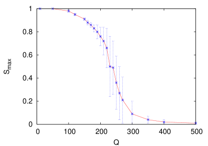
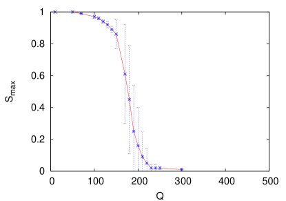
Figure 1: (Color online) Relative size of the largest cultural component $S_{max}$ of the final absorbing state as a function of the number $Q$ of cultural traits per feature. The diagrams are shown for SF (top) and ER (bottom) networks for comparison. In both cases we use $N=10^{3}$, $\langle k\rangle=6$ and $F=10$. The statistic is performed over $100$ realizations for each value of $Q$.

Iterating the above discrete-time dynamics for a number of time steps the system reaches a state in which all the links are blocked. In other words, the dynamics ends up in an absorbing state in which each pair of neighboring agents have cultures that are either identical or completely different. In general, in these absorbing states the network is fragmented into cultural clusters of identical individuals separated by borders composed of links having $S_{ij}=0$. The important situation in which all the nodes of the network are culturally identical is thus a subset of the total number, $q^{F}$, of absorbing states. In order to characterize the final state of the system, it is useful to measure the disorder of the corresponding absorbing state. A useful order parameter Castellano00 is the relative size of the largest cultural cluster, $S_{max}$. In one extreme case of global cultural consensus, this quantity takes the value $S_{max}=1$. In the other extreme situation in which all individuals are totally different from their neighbors, we have $S_{max}=1/N$.

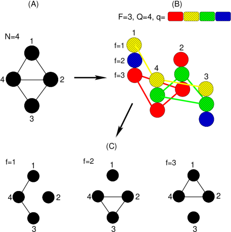
Figure 2: (Color online) Scheme of the feature level analysis. Starting from a network of $N=4$ nodes (A) and an Axelrod dynamics with $F=3$ and $Q=4$ we stop the dynamics at some time $t$ in which the cultural configuration is described in (B). For each of the $F=3$ cultural features we link those nodes that share the same trait. Finally, we obtain $F=3$ subnetworks (C) showing the consensus patterns for each cultural feature.

According to previous studies on square lattices, when $F>2$, a non-equilibrium first-order phase transition from order to disorder is observed as a function of the number of traits $Q$ (the control parameter of the phase transition) Castellano00 . In particular, the system always ends up in an ordered absorbing state ($S_{max}\sim 1$) when $Q<Q_{c}$ whereas for $Q>Q_{c}$ fragmented or disordered absorbing states ($S_{max}\ll 1$) trap the dynamics of the system. In finite complex networks, the picture is similar to the case of square lattices, although the observed value of $Q_{c}$ is larger Klemm3 . This finding points out that network shortcuts favor ordered states. To show the importance of the degree of heterogeneity of the substrate graph, we have used the model introduced in GomezMoreno to construct heterogeneous SF networks with $\gamma=3$, and homogeneous Erdös-Rényi (ER) graphs (i.e networks with $P(k)$ following a Poisson distribution ER ) with the same average connectivity $\langle k\rangle$. In Figure 1 we plot the curve $S_{max}(Q)$ for both ER and SF networks of $N=10^{3}$ nodes and $\langle k\rangle=6$. In both cases we have fixed the number of cultural features to $F=10$ and the results are averaged over $100$ different realizations of initial conditions and networks realizations. From the plots it is clear that in both cases the cultural consensus decreases as the number of possible traits increases. However, the order-disorder transition is seen to occur more sharply in the case of ER networks where the fluctuations around the transition region are remarkably higher than in the SF case as shown by the error bars. Besides, it is worth remarking that it has been found that in SF networks $Q_{c}(N)\sim N^{0.39}$, and thus in the thermodynamic limit the order-disorder transition disappears and only cultural consensus can be reached Klemm3 . Surprisingly, for what concerns the dynamical organization towards cultural consensus, we have not observed any qualitative difference between homogeneous and heterogeneous architectures. For this reason, in what follows, we will focus on the study of SF networks.

III Dynamical analysis at the feature level

Besides its critical behavior, the Axelrod model in regular lattices shows another remarkable feature: a non monotonic dynamics towards any of its frozen equilibria Castellano00 ; Redner . This non monotonicity refers to the time evolution of the number of active links, and is related to the fact that one interaction leading to consensus between two agents may simultaneously destroy a higher local consensus among one of these agents and the rest of its neighborhood sociophysics . This competition, due to the one-to-one nature of the interaction, leads to extremely large time scales to reach the final equilibrium in which all the links are blocked. Therefore, it is interesting to study in detail how this dynamical organization takes place in the case the model is implemented on a complex network $G$. To this end, we analyze the formation of cultural clusters, by looking at this process as the growth, link by link, of a network of “dynamical links”. We name $G(t)$ such a dynamical network at time $t$. We assume that a dynamical link $i-j$ between two connected (in $G$) individuals $i$ and $j$ is present in $G(t)$ if the two connected individuals are culturally identical at time $t$. The dynamical network $G(t)$ allows to characterize the transient dynamics of the Axelrod model towards the absorbing final state by means of the time evolution of network measures such as the number of cultural clusters in $G(t)$, the size of the largest cultural component, or the degree distributions of $G(t)$. In addition to this, we will also analyze the dynamical graph $G(t)$ as composed of $F$ different dynamical subnetworks, $G^{f}(t)$, $f=1,\ldots,F$, one dynamical subnetwork for each cultural feature. For a given feature $f$, the graph $G^{f}(t)$ is defined by considering two neighboring nodes $i$ and $j$ linked in graph $G^{f}(t)$ if they share at time $t$ the same cultural trait: $v_{i}^{f}=v_{j}^{f}$. Obviously, two neighbors can share a maximum of $F$ links, one for each feature, meaning that the two nodes have become culturally identical, $S_{ij}=1$.

In Fig. 2 we show how the graphs $G(t)$ and $G^{f}(t)$ are constructed in the case of a small graph $G$. We consider the network $G$ with $N=4$ nodes shown in Fig. 2.a), and the Axelrod model with $F=3$ cultural features and with $Q=4$ possible cultural traits. Suppose, at a given time $t$, the nodes of the network take the cultural configuration shown in Fig. 2.b). Then, the dynamical graph $G(t)$ has no links, while the three graphs $G^{f}(t)$, with $f=1,2,3$, are shown in (Fig. 2.c). Note that no couple of nodes in the system is culturally identical from the point of view of the order parameter $S_{max}$. Conversely, Fig. 2.c show that a certain internal consensus is observed at the level of each of the three features. In fact, connected components of size $3$ appear in each of the $F=3$ subnetworks. Summing up, the analysis we propose allows to observe the internal dynamical organization of the system by separating the processes that occur at each single cultural feature level, instead of integrating all the information into one single observable.

IV Results

The dynamics of the Axelrod model always ends up in a frozen state, a state in which no more changes are observed. As shown in Fig. 1, it depends on the value of $Q$ whether or not such a frozen state corresponds to a monocultural regime. In this Section we focus our attention on the dynamical evolution towards the frozen state. In order to properly analyze the time evolution of a generic quantity $X$ (such as the number of clusters, the average size of the largest component, etc), we need to average the results over a large number $R$ of trajectories. In particular, we have used at least $R=50$ different realizations for each value of $Q$. Since each initial condition can take a different time $T_{r}$ ($r=1$, …,$R$) to converge to the frozen state, the averaged evolution is obtained by mapping the time $t$ for each realization to a common normalized time $\tau=t/T_{r}$. Therefore, the corresponding averaged time evolution for the quantity $X$ is obtained as:

$$X(\tau)=\frac{1}{R}\left[\sum_{r=1;\;t/T_{r}=\tau}^{r=R}X_{r}(t)\right]\;.$$ (2)

Obviously, the averaged time evolution starts at $\tau=0$ and ends at $\tau=1$. For each initial realization we have stored the instant configurations of the network states so that we can easily measure the evolution of different topological quantities both at the global and at the feature level. For each realization $r$, the instant value of the quantity $X$ at the feature level, is denoted as $X^{f}_{r}(t)$ and corresponds to averaging over the values of $X$ for each of the $F$ features:

$$X^{f}_{r}(t)=\frac{1}{F}\sum_{j=1}^{F}X^{f}_{r,j}(t)\;,$$ (3)

where $X^{f}_{r,j}(t)$ is the value of $X$ at time $t$, for the realization $r$, and at the level corresponding to feature $j$ . Finally, in order to obtain the averaged time evolution $X^{f}(\tau)$, we average over the $R$ different realizations by using the normalized time $\tau$, as shown above in eq. 2.

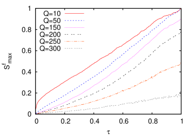
Figure 3: (Color online) Time evolution of the size of the largest cultural component, $S_{max}$, at the feature (top) and at the global (bottom) levels. We have considered SF networks with $N=10^{3}$ and $\langle k\rangle=6$ and $F=10$. The statistics is performed over $50$ different realizations.

The first measure we consider is the size of the largest component linking culturally identical individuals, both at the global, $S_{max}(\tau)$, and at the feature level, $S^{f}_{max}(\tau)$. Obviously, to compute $S^{f}_{max}$ we take, for each feature, the largest component connecting individuals sharing the same cultural trait of the corresponding cultural feature. In Fig. 3 we show the time evolution of $S_{max}$ and $S^{f}_{max}$ for several values of $Q$. The results point out that the largest component measured at the feature level grows very fast and that it reaches high values even when $S_{max}$ is still close to zero. In other words, when the largest component measured at the global scale starts growing, there are already a number of features in which consensus has been reached, and therefore a large number of nodes (if not all) are connected across these features. This behavior indicates that, despite the fact that there is no signal of global consensus, a macroscopic consensus already exist at the level of single features.

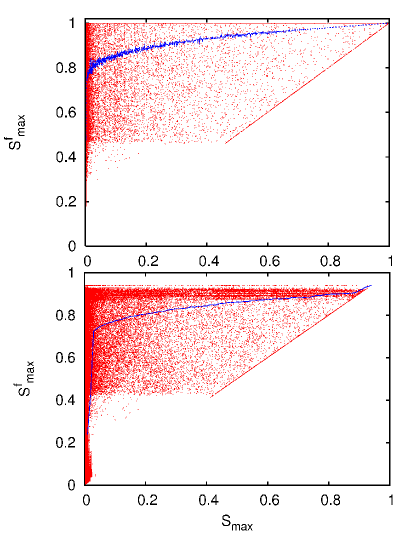
Figure 4: (Color online) The panels show the values (dots) of the largest cultural component of a single feature as a function of the size of the largest global consensus at the same time $(S_{max}^{f})_{r,j}(t)[(S_{max})_{r}(t)]$ found during the dynamical evolution of the Axelrod model in SF networks with $F=10$. We represent the evolution of the different features ($j=1,...,F$) for different realizations ($r=1,...,100$). The top and bottom panels correspond to $Q=20$ and $Q=150$, respectively. Both plots show that although most of the features have reached their own cultural consensus in a fast way there are few features (typically one for each realization) that considerably delay the global consensus of the system. Finally the solid (blue) line represents the average size of the largest cultural component at the feature level $S_{max}^{f}$ as a function of the size of the largest global consensus component $S_{max}$.

Figure 3 shows the average size of the largest cultural clusters at the feature level by averaging across the different $F$ features and realizations. From this figure it becomes evident that most of the features reach intra-cultural consensus in a time-scale much faster than that observed for the global consensus. On the other hand, the long transient dynamics towards global consensus of each realization of the Axelrod dynamics has its roots in the reorganization processes that occur inside each of the feature levels. Then, how does the fast organization of the averaged feature dynamics fit with the long transient observed at the global level? To answer this question it is convenient to look at the evolution of each cultural feature in a single realization of the Axelrod dynamics. In Figure 4 we show a scatter plot made up with the simultaneous values of the size of the global consensus cluster and that for the consensus cluster inside single features at different stages of the transient dynamics. In particular, we have plotted those couples of values $[(S_{max})_{r},(S_{max}^{f})_{r,j}]$ (where $r=1,...,R$ and $j=1,...,F$) observed at different time steps of the dynamics on SF networks for two different $Q$ values ($20$ and $150$). From the plot, it is clear that at the feature level there is a separation into fast and slow cultural features. The former features are identified, on the one hand, by the accumulation of dots close to $(S_{max}^{f})_{r,j}=1$ ($Q=20$) and $(S_{max}^{f})_{r,j}=0.9$ ($Q=150$) and, on the other hand, by the large values of the solid (blue) curve, $S_{max}^{f}(S_{max})$, constructed by averaging over the values $(S_{max}^{f})_{r,j}$ corresponding to the same value of $S_{max}$. In addition, the slow features have their fingerprint in the accumulation of dots along the line $S^{f}_{max}=S_{max}$ for high values of $S_{max}$. The separation into fast and slow features is not symmetric since, for each realization, most of the features belong to the fast group (as pointed out by the curve $S^{f}_{max}(S_{max})$) whereas few of them (typically $1$ as observed from the simulations) correspond to the slow group.

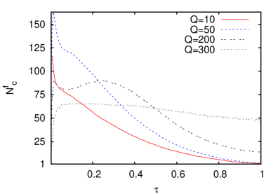
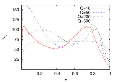
Figure 5: (Color online) Number of monocultural clusters in SF networks as a function of time at the feature, $N^{f}_{c}$, (top) and global, $N_{c}$, (bottom) levels. The time has been normalized as in Fig. 3. At the macroscopic level, the evolution of $N_{c}$ is not monotonous while at the feature level, and for those values of $Q$ for which final consensus is possible, the evolution of $N_{c}^{f}$ is dominated by a decreasing pattern. The networks have $N=10^{3}$ nodes, with $\langle k\rangle=6$ and $F=10$. For the $N_{c}$ figure, every point shown is the average over $50$ different realizations, while for the $N_{c}^{f}$ one, yet an additional average over the $F$ features has been made.

As for the number of monocultural clusters, we have observed that the behavior at the feature and global levels are also distinct. Figure 5 shows the results obtained for the number of clusters in the SF network as a function of time for different values of the parameter $Q$. At the feature level, except for short times, the dynamics of the model leads to a monotonously decreasing number of clusters for those values of $Q$ leading to a final equilibrium where macroscopic consensus is reached. Conversely, no monotonous behavior for the number of clusters is observed at the macroscopic level. As a matter of fact, the initial evolution of $N_{c}$ is close to that observed for $N_{c}^{f}$: it starts growing for low values of $\tau$, reaches a maximum and starts to decrease. However, in the case of $N_{c}$, around the transition time from the non-consensus regime to a globally visible consensus (see Fig. 3), the number of clusters starts to grow again, yielding a new maximum, to finally fall down very fast. This trend of the global dynamics points out again the reorganization taking place before reaching the final equilibrium. Once again, this reorganization seems not to affect the equilibria at the feature level. However, these differences between feature and global levels are again understood when following the growth of the largest components for each feature in single realizations of the Axelrod dynamics. The typical evolution shows that those fast features reach consensus in short times, $\tau\ll 1$, while those slow features remain fragmented for a number of time steps before reaching consensus together with the global system. Therefore, the clear separation of time-scales at the feature level implies that, although most of the agents reach consensus for most of their features in a fast way, the existence of few bottleneck features is responsible for the long transient of the global dynamics. It is inside these slow features where the processes of reorganization occur while the remaining (large) fraction of fast features remain unaltered in the state of internal cultural consensus.

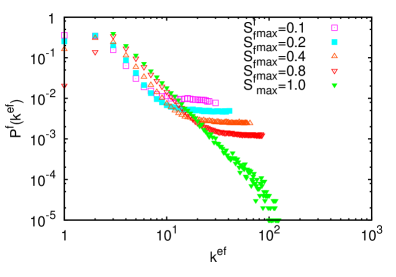
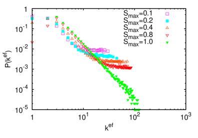
Figure 6: (Color online) Evolution with respect to the size of the largest component of the effective degree distributions as measured in the largest monocultural clusters at both feature (top) and global (bottom) levels of description in SF networks. The results correspond to $Q=10$ and indicate that hubs are always the latest to reach consensus. The networks we used have $N=10^{3}$ nodes, with $\langle k\rangle=6$ and $F=10$. For the $P(k)$ figure, every point shown is the average over $100$ different realizations, while for the $P^{f}(k)$ one, yet an additional average over the $F$ features has been made. See the main text for further details.

We can extract additional topological information using the approach adopted here. Usually, consensus models define a cultural pattern when the individuals that make up such pattern share all cultural traits. However, it is also possible that individuals relate to each other not because they share all the cultural features, but because they have one or several of these traits in common. Obviously, if we “look” at the system at a global level, we would be unable to detect cultural clusters unless the overlap between different individuals is one. As seen before, however, structures also emerge at the feature level. These “hidden” patterns can also be characterized topologically.

First we study the effective degree distribution of the giant consensus clusters, $P(k^{ef})$. The effective degree, $k_{i}^{ef}$, of a node $i$ belonging to a consensus cluster at the feature level is defined as the number of its physical neighbors that share the same cultural trait for the corresponding feature. For the global cluster we consider only those links that join culturally identical nodes. The effective degree distributions are normalized to the number of nodes in the corresponding consensus components. In Fig. 6 it is shown the effective degree distributions for different values of $S_{max}$ and $S^{f}_{max}$ respectively. The number of possible traits is set to $Q=10$ so that cultural consensus is always the final frozen state. From the evolution of $P(k^{ef})$ as $S_{max}$ and $S_{max}^{f}$ grow, and taking as reference the cases when $S_{max}=S^{f}_{max}=1$, one notices that highly connected nodes are the latest to reach consensus with its neighbors. In particular, hubs appear overpopulating the intermediate effective degree-classes for low values of $S_{max}$ and $S_{max}^{f}$. As the consensus components increase so do the effective degrees of hubs and finally they reach their physical connectivity. Interestingly, there are no significant differences in the degree distributions measured if one follows a feature or the system as a whole. Note, however, that the values of $S_{max}$ are realized at different times $-$ one at the beginning (features) and the other (global) at the end of the Axelrod dynamics.

Finally, in Fig.7 we show the variation of the average path length with the size of the giant component at the feature and global levels. The behavior of this quantity supports the phenomenological picture previously described and allows to understand how the largest cluster grows. For small values of $S_{max}$ and $S^{f}_{max}$, just a few nodes distributed in many clusters have reached consensus and thus $\langle l\rangle\approx 1$. As $S_{max}$ and $S^{f}_{max}$ grow, so do $\langle l\rangle$ and $\langle l^{f}\rangle$, which implies that more nodes are added to the consensus clusters, but that a significant number of newcomers are only connected to one member of the consensus component. In other words, when $S_{max}$ is small, the consensus clusters (either global or at single features) grow in a tree-like manner thus not having many loops and consequently showing large paths connecting different nodes in these clusters. Remarkably, for small sizes of the global consensus component, $S_{max}$, the curve $\langle l\rangle$ presents three branches. The branch corresponding to the largest values of $\langle l\rangle$ has its roots in the first frustrated growth of the global consensus discussed in Fig. 5. The middle branch subsequent corresponds to the decrease of $S_{max}$ for intermediate values of $\tau$ (pointed out by the increase in the number of global clusters, $N_{c}$, in Fig. 5). Finally, the third and lowest branch of $\langle l\rangle$ is due to the second and final growth of $S_{max}$. The large slope of the first branch of $\langle l\rangle$ points out that the frustrated growth of the global consensus occurs in a more tree-like way than the final one. Further increase of $S_{max}$ and $S^{f}_{max}$ finally leads to an increase of the probability of incorporating nodes sharing more than one connection with the consensus component. Therefore, at this stage, the addition of new nodes to the consensus components implies that a large number of links are also incorporated into the giant consensus component and thus at this second stage the growth is dominated by the addition of new links. As for both levels of description, the difference relies on the relative sizes of the giant consensus component at which the maxima of $\langle l\rangle$ and $\langle l^{f}\rangle$ are attained and the dependence with $Q$. In particular, for those values of $Q$ leading to a final macroscopic consensus, the values of $S^{f}_{max}$ corresponding to these maxima of $\langle l^{f}\rangle$ increase with $Q$ whereas for global consensus the trend is the opposite. Obviously, as $Q$ grows the curves for both $\langle l\rangle$ and $\langle l^{f}\rangle$ show the same two maxima.

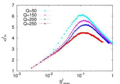
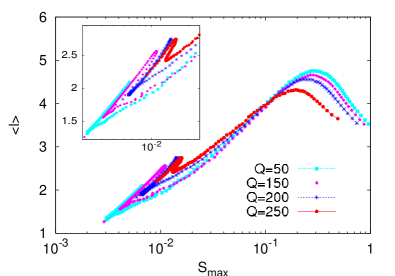
Figure 7: (Color online) Variation of the average path length of both representat ions with respect to the size of the corresponding giant components, $S_{max}^{f}$ (top) and $S_{max}$ (bottom), in SF networks and for different values of $Q$. The networks are made up of $N=10^{3}$ nodes, with $\langle k\rangle=6$ and $F=10$. For $\langle l\rangle$ the statistic is performed over $50$ different realizations, while for the $\langle l^{f}\rangle$, yet an additional average over the $F$ features has been made. The inset in the bottom plot shows in detail the region where the curve $\langle l\rangle(S_{max})$ is multivalued.

This different behavior for low values of $Q$ comes again from the existence of fast growing consensus clusters at the feature level: While the evolution of $\langle l\rangle$ is ruled by the (few) bottleneck features, $\langle l^{f}\rangle$ is mostly contributed by those fast growing features. As a consequence, the tree-like growth stage of the development of feature consensus clusters is replaced by the link-dominated growth much earlier than observed at the global level. This result points out again that the dynamical organization depends strongly on the level of representation of the dynamics.

V Conclusions

In this paper we have studied the microscopic dynamics towards cultural consensus in the Axelrod model on SF networks. In particular, we analysed how single traits spread across cultural features. Comparing such microscopic dynamics with that observed at the global level, i.e. integrating all the features into one cultural observable, we have shown that feature consensus is achieved remarkably faster than global consensus. In particular, while at the global level there are no signals of cultural consensus, most of the cultural features have already reached a macroscopic agreement. We have also observed important differences in the dynamic organization towards cultural consensus. In fact, at the global level there is a clear reorganization before cultural consensus is reached, this being evident from the non-monotonicity in the time evolution of the number of consensus clusters. Conversely, such reorganization processes are localized in a few cultural features rather than taking place in all the feature levels. Such localization points out the existence of a fast time scale for most of the cultural features which becomes screened when looking for the time evolution of the global consensus.

We have also analyzed the time evolution of the patterns of consensus clusters. In clusters defined both at single feature and at global scale, high degree, although present when macroscopic consensus is observed, show a misrepresented effective connectivity, since not all node neighbors are culturally identical. Additionally, the growth of a giant consensus components has two well-differentiated stages. In the first stage, the growth takes place in a tree-like manner, while in the second stage the nodes attracted come along with a large amount of links, reducing considerably the distances within these consensus clusters. Remarkably, at the feature level the tree-like growth is much shorter than the one dominated by the addition of links. This points out that the development of feature consensus clusters is more compact than its global counterpart.

Finally, it is worth stressing that we have not found any significant difference when applying the same analysis to homogeneous ER networks and lattice geometries, in contrast to other dynamical process where noticeable differences in the organization of the dynamical equilibria are observed s1 ; s2 ; Gomez-GardenesPRL ; Sinatra . This result poses an open question on the influence of network structure on the dynamical organization of the Axelrod model. For future work, it would be also interesting to design strategies that favor global consensus based on the existence of a fast time-scale for the development of consensus at the feature level of representation.

- (1) C. Castellano, S. Fortunato and V. Loreto, Rev. Mod. Phys. 81, 591 (2009).
- (2) R. Albert and A.-L. Barabási, Rev. Mod. Phys. 74, 47 (2002).
- (3) S. N. Dorogovtsev and J. F. F. Mendes, Adv. Phys. 51, 1079 (2002).
- (4) M. E. J. Newman, SIAM Review 45, 167 (2003).
- (5) S. Boccaletti, V. Latora, Y. Moreno, M. Chavez and D.-U. Hwang, Phys. Rep. 424, 175 (2006).
- (6) S.N. Dorogovtsev, A.V. Goltsev, and J.F.F. Mendes, Rev Mod. Phys. 80, 1275 (2008).
- (7) A. Arenas, A. Díaz-Guilera, J. Kurths, Y. Moreno and C. Zhou, Phys. Rep. 469, 93 (2008).
- (8) G. Szabó, and G. Fath, Phys. Rep. 446, 97 (2007).
- (9) R. Axelrod, J. Conflict Res. 41, 203 (1997).
- (10) R. Axelrod, The Complexity of Cooperation, (Princeton University Press, Princeton, 1997).
- (11) C. Castellano, M. Marsili, A Vespignani, Phys. Rev. Lett. 85, 3536 (2000).
- (12) J.C. González-Avella, V.M. Eguíluz, M.G. Cosenza, K. Klemm, J.L. Herrera and M. San Miguel, Phys. Rev. E 73, 046119 (2006).
- (13) K. Klemm, V.M. Eguíluz, R. Toral and M.San Miguel, Physica A 327, 1 (2003).
- (14) K. Klemm, V.M. Eguíluz, R. Toral, M. San Miguel, Phys. Rev. E 67, 045101 (2003).
- (15) C. Gracia-Lazaro, L. F. Lafuerza, L. M. Floría, and Y. Moreno, Phys. Rev. E 80, 046123 (2009).
- (16) D. Vilone, A. Vespignani, and C. Castellano, Eur. Phys. J. B 30, 399 (2002).
- (17) F. Vazquez, and S. Redner, Eur. Phys. Lett. 78, 18002 (2007).
- (18) K. Klemm, V.M. Eguíluz, R. Toral and M.San Miguel, Phys. Review E 67, 026120 (2003).
- (19) A.L. Barabási and R. Albert, Science 286, 509 (1999).
- (20) J. Gómez-Gardeñes and Y. Moreno, Phys. Rev. E 73, 056124 (2006).
- (21) P. Erdös and A. Rényi, Pub. Mathematicae 6, 290 (1959).
- (22) J. Gómez-Gardeñes, Y. Moreno, and A. Arenas, Phys. Rev. Lett. 98, 034101 (2007).
- (23) J. Gómez-Gardeñes, Y. Moreno, and A. Arenas, Phys. Rev. E 75, 066106 (2007). .
- (24) J. Gómez-Gardeñes, M. Campillo, L.M. Floría and Y. Moreno, Phys. Rev. Lett. 98, 108103 (2007).
- (25) R. Sinatra et al, J. Stat. Mech. P09012 (2009).