QCD Equation of State and Hadron Resonance Gas

Abstract

We compare the trace anomaly, strangeness and baryon number fluctuations calculated in lattice QCD with expectations based on hadron resonance gas model. We find that there is a significant discrepancy between the hadron resonance gas and the lattice data. This discrepancy is largely reduced if the hadron spectrum is modified to take into account the larger values of the quark mass used in lattice calculations as well as the finite lattice spacing errors. We also give a simple parametrization of QCD equation of state, which combines hadron resonance gas at low temperatures with lattice QCD at high temperatures. We compare this parametrization with other parametrizations of the equation of state used in hydrodynamical models and discuss differences in hydrodynamic flow for different equations of state.

I Introduction

Equation of state of hot strongly interacting matter play important role in cosmology hindmarsh ; laine and hydrodynamic description of heavy ion collisions kolb . In many cases hydrodynamical models which try to describe the collective flow in heavy ion collisions used equation of state (EoS) with first order phase transition, although lattice QCD shows that the transition to the deconfined phase is only a crossover nature . It is not obvious to what extent the collective flow is sensitive to details of the equation of state (EoS). It turns out, however, that in ideal fluid dynamics the anisotropy of the proton flow is particularly sensitive to the QCD equation of state pasi05 and using lattice inspired EoS with crossover transition overpredicts proton elliptic flow.

Attempts to calculate EoS on the lattice have been made over the last 20 years (see Refs. me ; carleton for reviews). One of the difficulties in calculating EoS on the lattice is its sensitivity to high momentum modes and thus to the effects of finite lattice spacing. This problem is particularly severe in the high temperature limit. Therefore in recent years calculations have been done using improved staggered fermions with higher order discretization of the lattice Dirac operators asqtad_eos ; p4_eos which largely reduce the cutoff dependence in the high temperature region. However, there is another source of discretization effects if staggered quarks are used. The staggered fermion formulation does not preserve the flavor symmetry of continuum QCD. Because of this the spectrum of low lying hadronic states is distorted and this may effect thermodynamic quantities in the low temperature region.

Hadron resonance gas (HRG) turned out to be very successful in describing particle abundances produced in heavy ion collisions PBM . It was also used to estimate QCD transport coefficients jaki as well as chemical equilibration rates johanna close to the transition temperature. Thermodynamic quantities calculated in lattice QCD with rather large quark mass agree well with the HRG model if the masses of the hadrons in the model are tuned appropriately to match the large quark mass used in lattice calculations redlich1 . Furthermore, the ratio of certain charge susceptibilities are not very sensitive to the details of the hadron spectrum and the lattice calculations of these ratios show a reasonably good agreement with HRG model predictions at low temperatures redlich2 ; redlich3 ; fluctuations . The purpose of this paper is to confront the results of recent lattice calculations performed with light quark masses with the prediction of the HRG model and clarify its range of applicability. As we will see the HRG model describes thermodynamic quantities quite well up to unexpectedly high temperatures. Therefore lattice EoS can be combined with HRG EoS at low temperatures to get rid of large discretization effects. Such an EoS is also useful for hydrodynamic modeling, and we construct a parametrization for an EoS interpolating between HRG at low temperatures and lattice QCD at high temperatures. The rest of the paper is organized as follows. In section II we discuss the hadron resonance gas model and the effects of finite lattice spacing on hadron masses. Section III deals with the comparison of fluctuations of baryon number and strangeness with the prediction of HRG model. In section IV we compare the HRG with the lattice results on trace anomaly and construct a parametrization of equation of state which is easy to use in hydrodynamic simulations. In this section we also give a detailed comparison with other parametrizations of EoS in the literature. In section V we discuss hydrodynamic flow for different EoSs discussed in the previous section, and highlight the differences. Finally section VI contains our conclusions. In appendices we discuss some technical aspects of the calculations, in particular the fits of the lattice data as well as the hydrodynamic flow for partial chemical equilibrium.

II Hadron resonance gas and lattice QCD

At sufficiently low temperature thermodynamics of strongly interacting matter at zero baryon number density is dominated by pions. The interaction between pions is suppressed and chiral perturbation theory can be used to estimate the pion contribution to thermodynamic potential gerber . In fact, for temperatures $T\leq 150$ MeV, the energy density of pions calculated in 3-loop chiral perturbation theory differs only by less than $15\%$ from the ideal gas value gerber . As temperature increases heavier hadrons start to contribute to thermodynamics. For temperatures $T\geq 150$MeV heavy states dominate the energy density. However, the densities of heavy particles are still small, $n_{i}\sim\exp(-M_{i}/T)$, and their mutual interactions, being proportional to $n_{i}n_{k}\sim\exp(-(M_{i}+M_{k})/T)$, are suppressed. Therefore one can use the virial expansion to evaluate the effect of interactions dashen . In the low temperature limit the virial expansion reduces to chiral perturbation theory gerber . The virial expansion together with experimental information on the scattering phase shifts was used by Prakash and Venugopalan to study thermodynamics of low temperature hadronic matter prakash . Their analysis showed that there is an interplay between attractive interactions (characterized by positive phase shifts) and repulsive interactions (characterized by negative phase shifts) such that their net effect can be well approximated by inclusion of free resonances : $\rho$, $K^{*}$, $\Delta(1234)$ etc. Thus the interacting gas of hadrons can be fairly well approximated by a non-interacting gas of resonances corroborating earlier ideas of the statistical bootstrap model hagedorn . To summarize, the partition function of strongly interacting matter at low temperature can be well approximated by the partition function of non-interacting hadrons and resonances

$$p^{HRG}/T^{4} = \frac{1}{VT^{3}}\sum_{i\in\;mesons}\ln{\cal Z}^{M}_{m_{i}}(T,V,\mu_{X^{a}})$$ (1)

$$+\frac{1}{VT^{3}}\sum_{i\in\;baryons}\ln{\cal Z}^{B}_{m_{i}}(T,V,\mu_{X^{a}})\;,$$

where

$$\ln{\cal Z}^{M/B}_{m_{i}}=\mp\frac{Vd_{i}}{{2\pi^{2}}}\int_{0}^{\infty}dkk^{2}\ln(1\mp z_{i}e^{-\varepsilon_{i}/T})\quad,$$ (2)

with energies $\varepsilon_{i}=\sqrt{k^{2}+m_{i}^{2}}$, degeneracy factors $d_{i}$ and fugacities

$$z_{i}=\exp\left((\sum_{a}X_{i}^{a}\mu_{X^{a}})/T\right)\;.$$ (3)

Here we consider all possible conserved charges $X^{a}$, including the baryon number $B$, electric charge $Q$, strangeness $S$ etc. We do not include any repulsive interactions in the form of excluded volume corrections or repulsive mean field Satarov .

The assumption that thermodynamics in the low temperature region is well described by a gas of non-interacting hadrons and resonances is important for practical applications of hydrodynamic models. At the end of the hydrodynamical evolution, the fluid is usually converted into particles using the Cooper-Frye procedure Cooper-Frye . This procedure conserves energy, momentum and charge without any specific considerations if, and only if, the equation of state of the fluid is the same than the equation of state of free particles Laszlo . Therefore it is important to confront the predictions of the hadron resonance gas for different thermodynamical quantities with the available lattice data.

The most extensive lattice calculations of the equation of state have been performed using two versions of improved staggered fermions: the so-called asqtad and p4 formulations asqtad_eos ; p4_eos ; hot_eos . Calculations have been performed using lattices with temporal extent $N_{\tau}=4$ and $6$ asqtad_eos ; p4_eos and more recently with temporal extent $N_{\tau}=8$ hot_eos . These correspond to lattice spacings $a=1/(4T)$, $1/(6T)$ and $1/(8T)$ respectively. The strange quark mass $m_{s}$ was close to its physical value, while the light ($u$ and $d$) quark masses were one tenth of the strange quark mass, $m_{q}=0.1m_{s}$, corresponding to the pion mass in the range $220-260$ MeV. The lattice calculations of the equation of state have been compared to the prediction of the hadron resonance gas p4_eos ; hot_eos . It turned out that the lattice results fall considerably below the HRG prediction. One obvious reason for this discrepancy is the fact that the quark mass used in lattice calculations is about a factor two larger then the physical one. However, this fact alone is unlikely to explain the whole discrepancy as the contribution of the pseudo-scalar mesons to the energy density is small and quark mass dependence of other hadron masses in this small quark mass region is relatively weak. On the other hand the lattice spacing dependence of the hadron masses may play an important role. Since the lattice calculations of the EoS are performed at fixed temporal extent $N_{\tau}$, the temperature is varied by changing the lattice spacing $T=1/(N_{\tau}a)$. As the temperature is decreased the lattice spacing gets larger and the cutoff effects on the hadron masses increase, i.e. the size of cutoff effects on the hadron masses is a function of the temperature.

The hadron masses for asqtad improved staggered fermions have been studied in Refs. bernard01 ; bernard04 ; bernard07 ; bazavov09 for several lattice spacings $a\simeq 0.06$, $0.09$, $0.125$, $0.18$ and $0.25$ fm. For all of these lattice spacings there are significant deviations in the hadron masses from the experimental values. Of course, after the proper continuum extrapolations all the hadron masses agree with the experiment bazavov09 . The large cutoff dependence of the hadron masses in the staggered formulation is due to large ${\cal O}(\alpha_{s}a^{2})$ discretization errors which also break the flavor symmetry. This is not the case for the improved Wilson fermion formulation Durr:2008a ; Durr:2008b , where cutoff dependence of the hadron masses is below $5\%$ already at lattice spacing $<0.2$fm. In the following subsections we discuss the cutoff dependence of the pseudo-scalar meson, vector meson and baryon masses separately.

II.1 Pseudo-scalar mesons in staggered formulation

The staggered formulation of lattice QCD describes four degenerate quark flavors in the continuum limit. To obtain the physical number of flavors, i.e. one relatively heavy strange quark and two light quarks, the so-called rooting procedure is used. The rooting procedure amounts to replacing the fermion determinant in the path integral expression of the partition function with its fourth root. In the continuum limit this procedure is justified continuum_root . At finite lattice spacing, however, the four flavors are not degenerate, but there are flavor changing discretization effects of order ${\cal O}(\alpha_{s}a^{2})$. As the result of this the sixteen pseudo-scalar mesons of the 4 flavor theory have unequal masses, and only one of them has a vanishing mass in the limit of the zero quark mass, $m_{q}\rightarrow 0$. The sixteen pseudo-scalar mesons can be grouped into eight multiplets golterman86 . The multiplets are characterized by the different masses $m_{{\rm ps}_{i}}$ and degeneracies $d_{\rm ps}^{i}$, $i=0,1,..7$. The first multiplet contains one Goldstone pseudo-scalar meson, i.e. $m_{{\rm ps}_{0}}^{2}\sim m_{q}$ and $d_{\rm ps}^{0}=1$. The flavor generators $\Gamma^{F}$ of the 4 flavor theory can be chosen to be the product of the Dirac matrices golterman86 ; kluberg . The masses of other pseudo-scalar mesons are given by

$$m_{{\rm ps}_{i}}^{2}=m_{{\rm ps}_{0}}^{2}+\delta m_{{\rm ps}_{i}}^{2}.$$ (4)

The quadratic splittings $\delta m_{ps_{i}}^{2}$ are independent of the input quark mass $m_{q}$ to a very good approximation and are proportional to $(\alpha_{s}a^{2})$ for small lattice spacings, and in general, increase with increasing index $i$. The correspondence between the index $i$ and the flavor matrix as well as the degeneracies $d_{\rm ps}^{i}$ for non-Goldstone pseudo-scalar mesons are given in Table 1.

The quadratic splittings have been calculated in numerical simulations with asqtad action in Refs. bernard04 ; bazavov09 . For lattice spacings $0.09{\rm fm}<a<0.25{\rm fm}$ the data can be well parametrized by the form

$$r_{1}^{2}\cdot\delta m_{ps_{i}}^{2}=\frac{a_{\rm ps}^{i}x+b_{\rm ps}^{i}x^{2}}{{(1+c_{\rm ps}^{i}x)}^{\beta_{i}}},~{}x=(a/r_{1})^{2}.$$ (5)

Here and in what follows we use the scale parameter $r_{1}$ extracted from the static quark potential $V(r)$ to convert from lattice units to physical units. The scale parameter $r_{1}$ is defined as

$$r^{2}\frac{dV(r)}{dr}|_{r=r_{1}}=1.0.$$ (6)

We use the value $r_{1}=0.318$ fm determined from bottomonium splitting bernard04 . The values of the parameters $a_{\rm ps}^{i}$, $b_{\rm ps}^{i}$, $c_{\rm ps}^{i}$, $\beta_{\rm ps}^{i}$ are given in Table 1.

i	$\Gamma^{F}$	$d_{\rm ps}^{i}$	$a_{\rm ps}^{i}$	$b_{\rm ps}^{i}$	$c_{\rm ps}^{i}$	$\beta_{\rm ps}^{i}$
1	$\gamma_{0}\gamma_{5}$	1	7.96583	45.6265	-0.983624	1.80
2	$\gamma_{i}\gamma_{5}$	3	25.9514	129.049	-4.673780	1.45
3	$\gamma_{i}\gamma_{j}$	3	19.3047	163.787	-5.675470	1.55
4	$\gamma_{i}\gamma_{0}$	3	4.26042	45.0193	-0.489748	2.00
5	$\gamma_{i}$	3	5.43308	79.455	-1.71669	2.00
6	$\gamma_{0}$	1	7.52963	95.2536	-2.24599	1.80
7	$1$	1	3.76433	70.8311	-0.373003	2.20

Table 1: The parameters of Eq. (5) describing the quadratic pseudo-scalar meson splittings. Also shown are the flavor matrices $\Gamma^{F}$ and the degeneracy factors $d_{\rm ps}^{i}$.

In Figure 1 we show the quadratic pseudo-scalar meson splittings calculated by the MILC collaboration bernard04 ; bazavov09 as function of the lattice spacing and compared with the parametrization given by Eq. (5). As one can see from the Figure 1, this parametrization gives good description of the data. In Figure 1 we also show the pseudo-scalar meson splitting for stout action used by the Budapest-Wuppertal group BW_Tc_09 . The splittings are significantly reduced compared to the calculations with asqtad action.

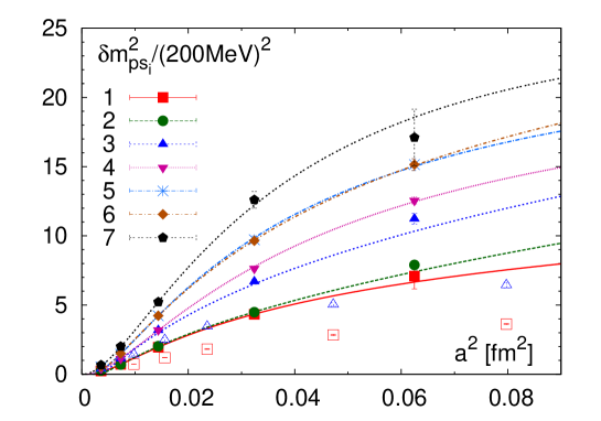
Figure 1: The quadratic splittings of non-Goldstone pseudo-scalar mesons in the seven different multiplets calculated with asqtad action bazavov09 at different lattice spacings. The lines show the parametrization given by Eq. (5). The open symbols refer to the lattice data obtained with the stout action BW_Tc_09 .

To take into account the flavor symmetry breaking in the pseudo-scalar meson sector, i.e. the fact that pion masses are non-degenerate the contributions of pions and kaons to the pressure is calculated as

$$p^{\pi,K}/T^{4}=\frac{1}{16}\frac{1}{VT^{3}}\sum_{i=0}^{7}d_{\rm ps}^{i}\ln{\cal Z}^{M}(m_{{\rm ps}_{i}}),$$ (7)

where $m_{{\rm ps}_{i}},~{}i=1-7$ is calculated according to Eq. (4) and $m_{{\rm ps}_{0}}$ is equal to the pion or kaon mass used in the actual lattice calculations. Figure 1 shows that the splitting between different pseudo-scalar mesons is quite large for lattice spacings used in calculations of the equations of state ($a=0.12-0.18$)fm. Even in the calculations with the stout action the mass of the heaviest pion that enters Eq. (7) is about $500$MeV if $N_{\tau}=8$ lattices are used. As the result the contribution of the pseudo-scalar mesons to thermodynamic quantities at finite lattice spacings is smaller than in the continuum.

II.2 Vector meson masses

In lattice calculations hadron masses are functions of the input quark mass and the lattice spacing. The quark mass dependence of the hadron masses is usually studied in terms of the lightest (Goldstone) pion mass. Since in lattice calculations quark masses are larger than the physical ones, and there is no full flavored chiral symmetry at finite lattice spacing a combined extrapolation in the pion mass and lattice spacing is needed for all hadron masses. We fitted the lattice spacing and pion mass dependence of the vector meson masses with the following simple formula

$$r_{1}\cdot m(a,m_{\pi})=r_{1}m^{phys}+\frac{a_{1}(r_{1}m_{\pi})^{2}-a_{1}(r_{1}m_{\pi}^{phys})^{2}}{1+a_{2}x}+\frac{b_{1}x}{1+b_{2}x},~{}x=(a/r_{1})^{2},~{}$$ (8)

where $m^{phys}$ is the physical value of the meson mass from the particle data book. It turns out that this formula describes the lattice spacing dependence of the vector meson masses in the interval $0.06{\rm fm}<a<0.18{\rm fm}$ for $(r_{1}m_{\pi})^{2}<0.8$. For strange vector mesons we set $a_{2}=0$ as there is no apparent lattice spacing dependence of the slope in their quark mass dependence. The numerical values of $a_{1},~{}a_{2},~{}b_{1}$ and $b_{2}$ are given in the Appendix A, where also the lattice data on the vector meson masses are shown.

II.3 Baryon masses

The nucleon and the $\Omega$ baryon masses have been calculated by the MILC collaboration with asqtad action at five different lattice spacings, $a=0.06,0.09,0.12$ and $0.18$fm bernard01 ; bernard04 ; bazavov09 ; milc_unpub and several quark masses. We performed a simultaneous fit of their quark mass (pion mass) and the lattice spacing dependence using the Ansatz given by Eq. (8), which works well for $(r_{1}m_{\pi})^{2}<0.8$. The parameters of this fit together with the lattice data on the nucleon and $\Omega$ baryon masses are presented in the Appendix A. In calculations with asqtad action the value of the strange quark mass was slightly larger than its physical value for each lattice spacing considered. This is due to the fact that the strange quark mass was fixed considering the ratio of the $\phi$ meson mass to the mass of the unmixed $\eta_{ss}$ pseudo-scalar meson instead fixing the kaon mass. This gives difference ${\cal O}(a^{2})$ in the value of the strange quark mass. To take this into account the lattice spacing dependence of the strange quark mass was parametrized as $m_{s}/m_{s}^{phys}(a)=1+1.02(a/r_{1})^{2}$. Then to estimate the $\Omega$ baryon mass we used the following formula

$$r_{1}m_{\Omega}(a,m_{\pi})=r_{1}m_{\Omega}^{phys}+a_{1}(r_{1}m_{\pi})^{2}-a_{1}(r_{1}m_{\pi}^{phys})^{2}+b_{1}x+(m_{\Omega}^{phys}-m_{\Delta}^{phys})\cdot 1.02x,~{}x=(a/r_{1})^{2}.$$ (9)

Here the last term accounts for the small deviation of the strange quark mass from its physical value. For other baryons ($\Delta$, $\Lambda$, $\Sigma$, and $\Xi$) no such detailed lattice calculations are available. Therefore to estimate the cutoff dependence of the $\Delta$ mass we use the same formula as for nucleon. While to estimate the cutoff dependence of the masses of the strange baryons we used the following formulas

$$\displaystyle r_{1}\cdot m_{\Lambda}(a,m_{\pi})=m_{\Lambda}^{phys}+\frac{2}{3}\frac{a_{1}(r_{1}m_{\pi})^{2}}{1+a_{2}x}+\frac{b_{1}x}{1+b_{2}x}+\frac{r_{1}\cdot(m_{\Lambda}^{phys}-m_{p}^{phys})}{1+a_{2}x}\left(\frac{m_{s}}{m_{s}^{phys}}\right),$$ (10)

$$\displaystyle r_{1}\cdot m_{\Sigma}(a,m_{\pi})=m_{\Sigma}^{phys}+\frac{1}{3}\frac{a_{1}(r_{1}m_{\pi})^{2}}{1+a_{2}x}+\frac{b_{1}x}{1+b_{2}x}+\frac{r_{1}\cdot(m_{\Sigma}^{phys}-m_{p}^{phys})}{1+a_{2}x}\left(\frac{m_{s}}{m_{s}^{phys}}\right),$$ (11)

$$\displaystyle r_{1}\cdot m_{\Xi}(a,m_{\pi})=m_{\Xi}^{phys}+\frac{1}{3}\frac{a_{1}(r_{1}m_{\pi})^{2}}{1+a_{2}x}+\frac{b_{1}x}{1+b_{2}x}+\frac{r_{1}\cdot(m_{\Xi}^{phys}-m_{p}^{phys})}{1+a_{2}x}\left(\frac{m_{s}}{m_{s}^{phys}}\right)$$ (12)

$$\displaystyle x=(a/r_{1})^{2}.$$

Here again we have taken into account that the strange quark mass in simulations with asqtad was slightly larger than the physical value. In the Appendix we give the comparison of the baryon masses calculated using the above formulas with available lattice results. It turns out that our parametrization of the baryon masses works reasonably well. We will use these parametrizations when calculating different quantities in the HRG model in the following sections.

III Fluctuations of conserved charges

Derivatives of the pressure with respect to chemical potential of conserved charges, e.g. baryon number ($B$), electric charge $Q$ and strangeness $S$ can be easily calculated in lattice QCD

$$\chi_{n}^{X}=T^{n}\frac{\partial^{n}p(T,\mu_{B},\mu_{Q},\mu_{S})}{\partial\mu_{X}^{n}}|_{\mu_{X}=0},~{}X=B,Q,S.$$ (13)

These are related to quadratic and higher order fluctuations of conserved charges $\chi_{2}^{X}=\langle X^{2}\rangle/(VT^{3})$, $\chi_{4}^{X}=(\langle N_{X}^{4}\rangle-3\langle N_{X}^{2}\rangle^{2})/(VT^{3})$ etc. Contrary to the pressure itself the evaluation of these derivatives does not involve zero temperature subtraction and integration in the temperature variable starting from some low temperature value. Therefore it is easy to compare them to the prediction of the HRG model. Different fluctuations up to the sixth order have been calculated for p4 and asqtad action fluctuations ; milcTc ; milc_lat09 on $N_{\tau}=4$ and $N_{\tau}=6$ lattices. Quadratic strangeness fluctuations have been also calculated on $N_{\tau}=8$ lattices for the p4 and asqtad actions by the HotQCD collaboration hot_eos . While there are extensive calculations with p4 action at finite temperature, the zero temperature hadron spectrum was not studied in detail for p4 action. Therefore our analysis of fluctuations and comparison with HRG model will mostly rely on results obtained with asqtad action.

Let us start our discussion with baryon number fluctuations. Baryon number fluctuations for asqtad action have been calculated in Ref. milcTc for $m_{q}=0.2m_{s}$ on $N_{\tau}=6$ lattices. Equations (8)-(12) describe the quark mass and lattice spacing dependence of ground state baryon masses calculated on lattice with asqtad action. Nothing is known about the lattice spacing dependence of the excited baryon masses which play very important role in baryon number fluctuations in the temperature range of interest. We assume that all the excited baryons up to certain mass threshold $m_{cut}^{B}$ have the same quark mass and lattice spacing dependence, while the baryon masses above that threshold are not modified by finite lattice spacing. The mass threshold $m_{cut}^{B}$ is an additional parameter of our model. In Fig. 2 we show the lattice data for baryon number fluctuations for asqtad action compared with hadron resonance gas model with physical value of the baryon masses including all the states up to $2.5$GeV. The lattice data fall considerably below the HRG prediction. The baryon number fluctuations have also been calculated in a HRG model, where all the baryon masses up to the $m_{cut}^{B}=1.8$GeV and $m_{cut}^{B}=2.5$GeV have been modified according to Eqs.(8)-(12) . The corresponding results are shown as dashed lines. As one can see, the HRG overshoots the lattice data with $m_{cut}^{B}=1.8$GeV, while with $m_{cut}^{B}=2.5$GeV it undershoots the lattice data. However, the agreement between lattice data and HRG is greatly improved. For completeness we also show the lattice data for p4 action calculated for $m_{q}=0.1m_{s}$ fluctuations .

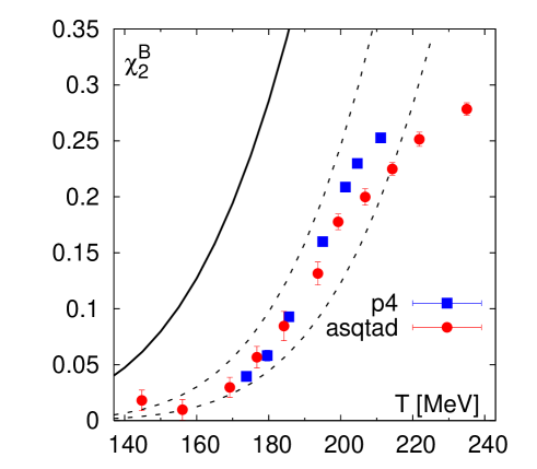
Figure 2: Baryon number fluctuations calculated with asqtad action on the $N_{\tau}=6$ lattices compared with HRG model with physical value of the baryon masses (solid line) and with HRG model with baryon masses calculated according Eqs. (8)-(12), $m_{cut}^{B}=1.8$GeV and $m_{cut}^{B}=2.5$GeV (dashed lines). Also shown are the lattice results for the p4 action.

Strangeness fluctuations have also been calculated on the lattice using asqtad and p4 action fluctuations ; hot_eos ; milcTc ; milc_lat09 on $N_{\tau}=6$ and $N_{\tau}=8$ lattices. We have calculated strangeness fluctuations in HRG model, where ground vector state meson masses have been calculated using Eq. (8), while baryon masses have been calculated using Eqs. (8)-(12). The contribution of kaons has been treated in the way discussed in section II.1, i.e. for each physical kaon averaging over sixteen staggered flavors have been performed and the mass splitting has been calculated using Eq. (5). This turns out to be important for the description of strangeness fluctuation for temperatures $T<165$MeV, where the contribution of kaons is quite significant. In Fig. 3 we show the prediction of the HRG model with modified hadron masses compared to the lattice data for asqtad action for $N_{\tau}=8$. In the figure we show the prediction of the HRG model with cutoffs $m_{cut}^{B}=1.8$GeV and $m_{cut}^{B}=2.5$GeV for the baryon masses. Here the effect of using different cutoffs for the modification of the baryon masses is significantly smaller as meson contribution to strangeness fluctuations is large. In the figure we also show the prediction of the HRG model with physical hadron masses as well as the lattice results for the p4 action. As one can see the lattice data fall significantly below the predictions of HRG model with physical quark masses, while the HRG model with modified hadron masses gives quite a good description of the lattice data. For completeness we also show the result for HRG model with modified hadron masses for $N_{\tau}=12$.

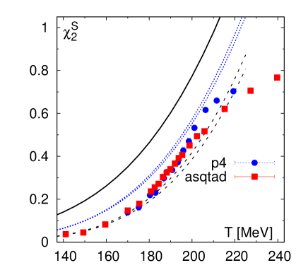
Figure 3: The strangeness fluctuations calculated on $N_{\tau}=8$ lattices for asqtad and p4 actions and compared with the prediction of the HRG model with physical (solid line) and modified (dashed lines) hadron masses. The upper (lower) dashed line corresponds to $m_{cut}^{B}=1.8(2.5)$GeV. The doted lines show the prediction of the HRG with modified hadron masses for $N_{\tau}=12$.

As one can see from Figs. 2 and 3, HRG model can describe baryon number and strangeness fluctuations reasonably well up to temperatures as high as $T_{c}$.

IV QCD equation of state

IV.1 The trace anomaly and parametrization of the equation of state

Available lattice data provide an EoS which is not easy to use in hydrodynamic models because different thermodynamic quantities are suppressed in the low temperature region due to discretization errors. In the previous section we have seen this for baryon number and strangeness fluctuations.

In lattice QCD the calculation of the pressure, energy density and entropy density usually proceeds through the calculation of the trace anomaly $\Theta(T)=\epsilon(T)-3p(T)$. Using the thermodynamic identity the pressure difference at temperatures $T$ and $T_{\rm low}$ can be expressed as the integral of the trace anomaly

$$\frac{p(T)}{T^{4}}-\frac{p(T_{\rm low})}{T_{\rm low}}=\int_{T_{\rm low}}^{T}\frac{dT^{\prime}}{{T^{\prime}}^{5}}\Theta(T).$$ (14)

By choosing the lower integration limit sufficiently small, $p(T_{\rm low})$ can be neglected due to the exponential suppression. Then the energy density $\epsilon(T)=\Theta(T)+3p(T)$ and the entropy density $s(T)=(\epsilon+p)/T$ can be calculated. This procedure is known as the integral method boyd . Since the trace anomaly plays a central role in lattice determination of the equation of state, we will discuss it in the HRG model and its comparison with the lattice data in the following. As we will see this helps constructing realistic equation of state that can be used in hydrodynamic models.

As mentioned before, finite temperature lattice calculations are usually performed at fixed temporal extent $N_{\tau}$ and the temperature is varied by varying the lattice spacing $a$, $T=1/(N_{\tau}a)$. Thus, calculations at low temperatures are performed on coarse lattices, while the lattice spacing gets smaller as the temperature is increased. Consequently the trace anomaly can be accurately calculated in the high temperature region, while in the low temperature region it is affected by possibly large discretization effects. Therefore to construct realistic equation of state we could use the lattice data for the trace anomaly in the high temperature region, $T>250$MeV, and use HRG model in the low temperature region, $T\mathrel{\lower 3.87495pt\hbox{$\stackrel{{\scriptstyle\displaystyle<}}{{\sim}}$}}180$ MeV. In Fig. 4 we compare the lattice results on trace anomaly obtained on $N_{\tau}=8$ lattices with asqtad and p4 action with the HRG model.

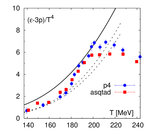
Figure 4: The trace anomaly calculated in lattice QCD compared with the HRG model with physical hadron masses (solid line) and modified hadron masses (dashed lines). The upper (lower) dashed line corresponds to $m_{cut}^{B}=1.8(2.5)$GeV.

The HRG model with modified masses appears to describe the lattice data quite well up to temperatures of about $180$MeV. In the intermediate temperature region $180{\rm MeV}\mathrel{\lower 3.87495pt\hbox{$\stackrel{{\scriptstyle\displaystyle<}}{{\sim}}$}}T<250{\rm MeV}$ the HRG model is no longer reliable, whereas discretization effects in lattice calculations could be large. The later can be seen by comparing the lattice data obtained on $N_{\tau}=6$ and $N_{\tau}=8$ lattices with p4 and asqtad action. Therefore we constrain the trace anomaly in the intermediate region only by the value of the entropy density at high temperatures.

In pure gauge theory, where continuum extrapolation has been performed, the entropy density falls below the ideal gas limit only by $15\%$ at temperatures of about $4T_{c}$ boyd ($T_{c}$ is the transition temperature). In QCD the entropy density calculated on $N_{\tau}=6$ and $8$ lattices is $(5-10)\%$ below the ideal gas limit petr_qm09 at the highest available temperature. Furthermore, resummed perturbative calculations describe quite well the entropy density in the high temperature region both in pure gauge theory blaizot and in QCD petr_qm09 . These calculations indicate that deviation from the ideal gas limit is about $(5-10)\%$. The fluctuations of quark number are also close to ideal gas limit and well described by resummed perturbative calculations petr_qm09 . Here the deviation from the ideal gas limit is less than $5\%$. Therefore we will use the guidance from existing lattice QCD calculations and require that the entropy density is below the ideal gas limit by either $5\%$ or $10\%$, when parametrizing the trace anomaly.

At high temperature the trace anomaly can be well parametrized by the inverse polynomial form (see e.g. Ref. hot_eos ). Therefore we will use the following Ansatz for the high temperature region

$$(e-3P)/T^{4}=d_{2}/T^{2}+d_{4}/T^{4}+c_{1}/T^{n_{1}}+c_{2}/T^{n_{2}}.$$ (15)

This form does not have the right asymptotic behavior in the high temperature region, where we expect $(e-3P)/T^{4}\sim g^{4}(T)~{}1/\ln^{2}(T/\Lambda_{QCD})$, but works well in the temperature range of interest. Furthermore, it is flexible enough to do the matching to the HRG result in low temperature region. We match to the HRG model at temperature $T_{0}$ by requiring that the trace anomaly as well as its first and second derivatives are continuous. The parametrization of the trace anomaly and thus QCD equation of state obtained using these requirements are labeled by $s95p\rm{-v1}$, $s95n\rm{-v1}$ and $s90f\rm{-v1}$. The labels “$s95$” and “$s90$” refer to the fraction of the ideal entropy density reached at $T=800$MeV ( 95% and 90% respectively), whereas the labels $p$, $n$ and $f$ refer to a specific treatment of the peak of the trace anomaly or its matching to the HRG. The detailed procedure of performing the fit to the lattice data and matching to the HRG model is described in Appendix B, where also the labeling scheme is explained in more detail. The values of the parameters $T_{0},~{}d_{2},~{}d_{4},~{}c_{1},~{}c_{2},~{}n_{1}$ and $n_{2}$ in each parametrization are given in Table 2.

	$d_{2}$ (GeV2)	$d_{4}$ (GeV4)	$c_{1}$ (GeV${}^{n_{1}}$)	$c_{2}$ (GeV${}^{n_{2}}$)	$n_{1}$	$n_{2}$	$T_{0}$ (MeV)
$s95p$	0.2660	2.403$\cdot 10^{-3}$	-2.809$\cdot 10^{-7}$	6.073$\cdot 10^{-23}$	10	30	183.8
$s95n$	0.2654	6.563$\cdot 10^{-3}$	-4.370$\cdot 10^{-5}$	5.774$\cdot 10^{-6}$	8	9	171.8
$s90f$	0.2495	1.355$\cdot 10^{-2}$	-3.237$\cdot 10^{-3}$	1.439$\cdot 10^{-14}$	5	18	170.0

Table 2: The values of the parameters for different fits of the trace anomaly.

The HRG result for the trace anomaly can also be parametrized by the simple form

$$\frac{\epsilon-3P}{T^{4}}=a_{1}T+a_{2}T^{3}+a_{3}T^{4}+a_{4}T^{10},$$ (16)

with $a_{1}=4.654$ GeV^-1, $a_{2}=-879$ GeV^-3, $a_{3}=8081$ GeV^-4, $a_{4}=-7039000$ GeV^-10 (see Appendix B for details).

The lattice data for trace anomaly compared to the parametrization given by Eqs. (15) and (16) is shown in Fig. 5. We show three parametrizations in the figure corresponding to a entropy density at $T=800$MeV which is below the ideal gas limit by $5\%$ ($s95p\rm{-v1}$ and $s95n{\rm-v1}$, the solid and dotted lines, respectively) and $10\%$ ($s90f\rm{-v1}$, dashed line). All the parametrizations describe the lattice data for $T>250$MeV, while in the low temperature region, $T<170$MeV, they are significantly above the lattice results. On the other hand, our parametrizations of the trace anomaly are below the lattice data in the peak region. This comes from the imposed constraint on the entropy density at $T=800$MeV. If we would use a parametrization which goes through the $N_{\tau}=8$, p4 lattice data and matches the resonance gas model at some temperature near $190$MeV, the entropy density would overshoot the ideal gas limit already at temperatures of about $600-700$MeV. Such a behavior would contradict the available lattice and weak coupling results.

The difference in the $s95n\rm{-v1}$ and $s95p{\rm-v1}$ parametrizations is in the treatment of the peak region. When we do the fit only on the lattice data above $T=250$MeV ($s95n{\rm-v1}$, dotted line), the peak value is clearly below the present data. To explore the sensitivity of the EoS to the height of the peak, we also did the fit using one additional point at $T=205$MeV close to the present data, and the same entropy constrain ($s95p{\rm-v1}$, solid line). This forces the trace anomaly almost to reach the data at the peak maintaining a reasonable fit to the data at high temperatures.

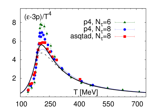
Figure 5: The trace anomaly calculated in lattice QCD with p4 and asqtad actions on $N_{\tau}=6$ and $8$ lattices compared with the parametrization given by Eqs. (15) and (16). The solid, dotted and dashed lines correspond to parametrizations $s95p{\rm-v1}$, $s95n{\rm-v1}$ and $s90f\rm{-v1}$ respectively, as discussed in the text.

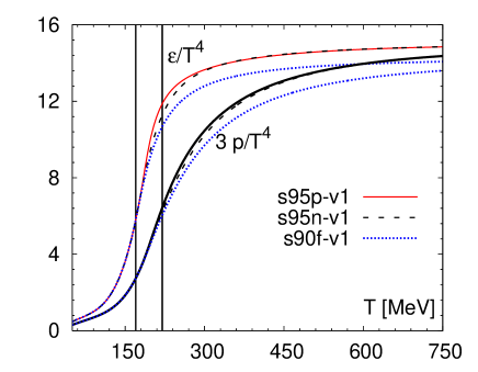
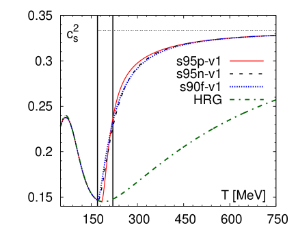
Figure 6: The pressure, energy density (left panel) and speed of sound (right panel) in the equations of state obtained from Eqs. (15) and (16). The vertical lines indicate the transition region (see text). In the right panel we also show the speed of sound for the HRG EoS and EoS with first order phase transition (thin dotted) line, the EoS Q

The EoSs, obtained by integrating the parametrizations given in Eqs. (15) and (16) over temperature as shown in Eqs. (14), are shown in Fig. 6. The clearest difference between our different parametrizations is trivial: The different behavior at high temperatures is due to the different entropy constraint at $T=800$MeV, which is of course manifested in energy density and pressure too. On the other hand, the different height of the peak of the trace anomaly causes only a tiny difference in pressure and energy density around $T=200$ MeV. This difference is manifested much clearer in the speed of sound: The large peak and larger switching temperature from HRG to lattice causes much more rapid change in the speed of sound in $s95p{\rm-v1}$ parametrization than in the two others. One could claim that the differences in the speed of sound are due to the different matching temperatures $T_{0}$, but we want to remind the reader that we treated $T_{0}$ as a fitting parameter in our model, and any changes in $T_{0}$ would make the fit to the lattice data worse (see details in Appendix B). In Figure 6 we show the speed of sound for EoS Q from Refs. Kolb ; pasi07 : An equation of state with a first order phase transition at $T_{c}=170$MeV. Below $T_{c}$ EoS Q coincides with HRG EoS, while above this temperature it is given by bag equation of state with three massless flavors and bag constant $B=(0.2447GeV)^{4}$. Nevertheless, the most striking feature of the speed of sound in the proposed parametrization of the EoS is that there is no softening below the hadron gas. There is no region where speed of sound would be smaller than in hadron gas, and its minimum value is that of HRG speed of sound. It is quite simple to understand why this happens: To achieve smaller speed of sound than the speed of sound in hadron gas, the trace anomaly should be larger than in HRG. As one can see in Fig. 4, the present lattice data clearly disfavors such a scenario. In Figure 6 we indicate the transition region from hadronic matter to deconfined state by vertical lines. We define the transition region as the temperature interval $170{\rm MeV}<T<220{\rm MeV}$. In view of the crossover nature of the finite temperature QCD transition such definition is ambiguous. The lower temperature limit in our definition comes form the fact that for $T<170$MeV all our EoS agree with HRG EoS. The rapid rise in the energy density and entropy density stops roughly at $220$MeV and starting from this temperature the variation of thermodynamic quantities is quite smooth hot_eos . Also the Kurtosis of the baryon number becomes compatible with quark gas at temperatures of about $220$MeV fluctuations . For these reasons we have chosen it as the upper limit for the transition region.

IV.2 Comparison with other works

The idea of using HRG in low temperatures and parametrized lattice EoS in high temperatures is by no means new. Laine and Schröder constructed QCD equation of state based on the effective theory approach in the high temperature region, while using the resonance gas equation of state in the low temperature region LS . In the effective theory approach the contribution of hard modes is treated perturbatively, while the contribution of soft modes is calculated using 3 dimensional lattice simulations of the effective theory called EQCD eqcd . This parametrization has been used in recent recent viscous hydrodynamic calculations luzum . The smooth matching to the resonance gas was done in the temperature interval $T=170-180$MeV.

Two other parametrizations of the EoS chojnacki07 ; chojnacki08 ; heinz08 used lattice data of Budapest-Wuppertal(BW) group obtained using so-called stout staggered fermion action BW and temporal extent $N_{\tau}=4$ and $6$. Since the stout action does not use higher order difference scheme in the lattice Dirac operator, discretization effects at high temperatures are very large. In the ideal gas limit the pressure calculated on $N_{\tau}=4$ and $6$ lattices is about twice the continuum value. As the consequence the lattice results of the BW group have large cut-off effects and overshoot the continuum ideal gas at high temperatures, see discussion in Ref. petr_sewm06 . In an attempt to correct this problem the authors of Ref. BW divided all their thermodynamic observables by the corresponding ideal gas value calculated on $N_{\tau}=4$ and $6$. Since cutoff effects are strongly temperature dependent this procedure overestimates cutoff effects in the interesting temperature region and underestimates the pressure and other thermodynamic observables.

The Krakow group used the stout lattice results parametrized in Ref. bz with $T_{c}=167$MeV and matched the speed of sound to the HRG result at that temperature chojnacki07 ; chojnacki08 . The procedure of the Krakow group involves extracting all the other thermodynamical quantities from the speed of sound using the relation

$$s(T)=s(T_{0})\exp\left[\int_{T_{0}}^{T}\frac{dT^{\prime}}{T^{\prime}c_{s}^{2}}\right].$$ (17)

Connecting the speeds of sound in HRG and lattice leads in this procedure to a larger entropy density at high temperatures than given by the lattice parametrization of Ref. bz . To make their EoS to fit the lattice data at $T\approx 1$GeV, the Krakow group made the speed of sound smaller in the temperature region $28<T<118$ MeV by hand chojnacki . This change is below the expected freeze-out temperature, and thus the speed of sound which affects the actual hydrodynamical evolution is unchanged. However, since entropy density is calculated by integrating over the entire temperature range, entropy density is smaller than the original HRG value everywhere in the range $28\mathrm{MeV}<T<T_{c}$. More specifically, in the range $120<T<160$MeV, both energy and entropy densities and pressure are $\sim 5\%$ below the HRG value, and energy is not automatically conserved at freeze-out, see the discussion in section V.

Heinz and Song also used the BW lattice results, but they parametrized pressure and temperature as function of energy density and matched them to HRG result; they used $T_{c}=172$MeV heinz08 . As the authors themselves note, their EoS is not exactly thermodynamically consistent, which leads to a violation of entropy conservation in an ideal fluid calculation. However, to our understanding this does not affect the qualitative studies the EoS has been used so far and the conclusions of those papers should be valid.

Here a note concerning $T_{c}$ in these parametrizations is in order: In Ref. BW thermodynamic quantities are given as function of $T/T_{c}$ but the value of $T_{c}$ is not specified. At lattice spacings corresponding to temporal extent $N_{\tau}=4$ and $N_{\tau}=6$, used in BW EoS calculations, $T_{c}$ has large cutoff effects and may deviate considerably from the continuum value $T_{c}=170(3)(4)$MeV determined in Ref. BW_Tc_09 (e.g. calculations of $T_{c}$ reported at Quark Matter 2005 on $N_{\tau}=4$ and $6$ lattices gave $T_{c}=189(8)$MeV katz_qm05 ). The best way to eliminate part of the cutoff effects in the BW EoS is to use the continuum value of the transition temperature $T_{c}$, which is interestingly enough appears to agree within errors with the values used in the phenomenological parametrizations discussed above.

The parametrization of the EoS by the HotQCD Collaboration hot_eos is based on a simple fit of the lattice results on the trace anomaly. For temperatures below $130$MeV, where no lattice data is available, HRG values for the trace anomaly have been used and assigned an artificial error. The resulting parametrization is well below the HRG at temperatures $T>50$ MeV, see discussion in Ref. hot_eos . For example, at $T\approx 130$MeV and $T\approx 170$MeV temperatures, pressure, energy and entropy densities are roughly 20% and 10% smaller than in HRG, respectively. Therefore, when one uses this parametrization, energy conservation at freeze-out requires additional consideration, see the discussion in section V.

In the Fig. 7 we show the comparison of our parametrization for EoS with the ones discussed above including the trace anomaly, speed of sound, pressure and energy density as function of the temperature as well as the pressure as function of the energy density.

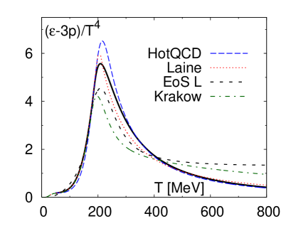
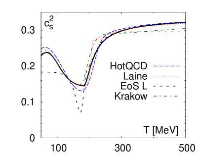
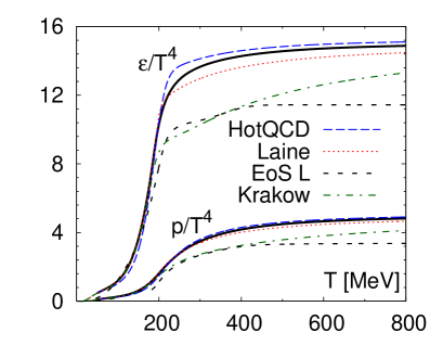
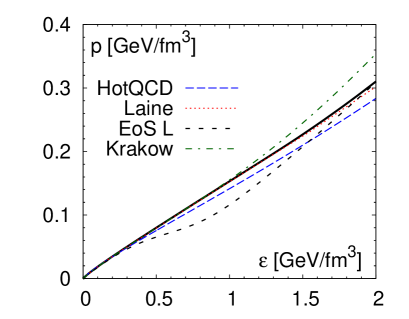
Figure 7: The trace anomaly, the speed of sound, the pressure and the energy density as function of the temperature for different parametrizations used in hydrodynamic models. Also shown is the the pressure as function of the energy density. The solid black line corresponds to s95p-v1 parametrization.

From the figure we see that there are significant differences between different parametrizations. The parametrization based on BW lattice results seem to have different high temperature asymptotic. In the low temperature region the EoS L parametrization by Heinz and Song and the HotQCD parametrization differ significantly from others. It is worth noting that EoS L does not even try to reproduce the HRG below 130 MeV temperature. The authors assumed that the details of the EoS below freeze-out temperature have only a negligible effect on the evolution within the freeze-out surface and a faithful reproduction of the HRG is thus not needed. Finally, for the trace anomaly, the difference between our parametrization and HotQCD parametrization is limited to temperatures $T<250$MeV by construction. However, since the pressure, energy density and entropy density is obtained using the integral method the differences in trace anomaly at low temperatures result in differences at all temperatures for these quantities.

V Effect on hydrodynamical flow

Now we are in a position to use the lattice results on EoS in a hydrodynamical model and compare the results with previous approaches using first order phase transition or the other lattice parametrizations in the literature. We also quantify how present uncertainties in the EoS parametrization affect the hydrodynamical flow. For simplicity we perform our analysis using ideal hydrodynamics. This is also motivated by the fact that the overall value and temperature dependence of the QCD and HRG transport coefficients is not known and any attempts to parametrize them would introduce additional uncertainties in the analysis.

As the first step we study the sensitivity of the momentum anisotropy $\epsilon_{p}$ on the EoS. This is the cleanest way to address the sensitivity of hydrodynamic flow to the EoS as additional complications due to freezeout do not enter here. The momentum anisotropy is defined as Kolb

$$\epsilon_{p}=\frac{\langle T_{xx}-T_{yy}\rangle}{\langle T_{xx}+T_{yy}\rangle},$$ (18)

where $T_{xx}$ and $T_{yy}$ are the diagonal transverse components of the energy-momentum tensor and brackets denote averaging over the entire transverse plane. In Figure 8 we show the time evolution of momentum anisotropy in Au+Au collisions at $\sqrt{s_{\mathrm{NN}}}=200$ GeV with $b=7$fm impact parameter for different EoSs. The left panel shows the anisotropy calculated using our different parametrizations, and EoS Q from Refs. Kolb ; pasi07 . As studied in detail in Ref. Kolb the first order phase transition causes the build up of the flow anisotropy to stall when most of the system is in the mixed phase. There is no such a structure when the transition to the hadronic matter is a smooth cross over, but the anisotropy increases monotonously. The hardness of the EoS in plasma phase is also manifested in the early behavior of the anisotropy. EoS Q is much harder in that region than any of the lattice EoSs studied here, and thus the build up of the flow anisotropy is faster. On the other hand, the mixed phase makes the EoS Q much softer in average during the evolution, and the final anisotropy is the smallest of all EoSs studied here. The speed of sound is quite similar in EoSs $s95p\mathrm{-v1}$, $s95n\mathrm{-v1}$ and $s90f\mathrm{-v1}$, and consequently the development of the flow anisotropy is similar. When the system cools, the speed of sound stays large longest for $s95p\mathrm{-v1}$, but it also drops fastest and stays small longest for $s95p\mathrm{-v1}$. These effects cancel, and the evolution of the anisotropy is almost identical to $s95n\mathrm{-v1}$. After that argument, the largest anisotropy obtained using $s90f\mathrm{-v1}$ may look surprising, but closer inspection of Fig. 6 reveals that $s90f\mathrm{-v1}$ has always either larger or equal speed of sound than $s95p\mathrm{-v1}$. Thus $s90f\mathrm{-v1}$ is harder, and it should lead to a larger anisotropy than $s95p\mathrm{-v1}$.

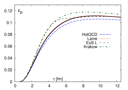
Figure 8: The time evolution of the momentum anisotropy in $b=7$ fm Au+Au collisions using the EoSs developed in this paper and the old EoS with a first order phase transition (EoS Q) from Ref. Kolb ; pasi07 (left panel) and the EoS $s95p\mathrm{-v1}$ compared to the various lattice EoSs in the literature LS ; chojnacki07 ; chojnacki08 ; heinz08 ; hot_eos (right panel). In the right panel the solid black line refers to the result obtained with $s95p\mathrm{-v1}$ parametrization. The inset in the right panel shows the temperature evolution in the middle of the system for different EoS. The horizontal lines indicate the transition region.

The old wisdom has been that elliptic flow builds up quickly during the early stages of the evolution and is mostly build up during the plasma phase. For example, for EoS Q, three quarters of the final anisotropy has been built up when the center of the system reaches mixed phase. For lattice based EoSs this is no longer as clear: Roughly half of the anisotropy is built up during the transition region, after the first three fm of the evolution, but the hadronic contribution from below $T=170$ MeV temperatures to $\epsilon_{p}$ is essentially negligible unlike in EoS Q. This difference in the evolution is partly explained by the softer EoS in the plasma phase—anisotropy is built up slower. Another reason is that the transition region in our EoSs reaches up to $\epsilon\approx 3.5$ GeV/fm³ energy density, whereas EoS Q reaches plasma phase already at $\epsilon\approx 2.15$ GeV/fm³ density.

In the right panel of Fig. 8 $s95p-\rm v1$ is compared to other lattice EoSs in the literature. The differences in flow are difficult to sort out based on the speed of sound as function of temperature alone, but they are easy to understand when one looks at the pressure as function of energy density (Fig. 7). It can be seen that the gradient $\partial P/\partial\epsilon$, i.e. speed of sound squared, is largest for the Krakow EoS, and EoS L is approximately as stiff as the Krakow EoS above $\epsilon\approx 1$ GeV/fm³ density. Thus it is not surprising that the Krakow EoS leads to the largest anisotropy, and that the initial build up of the anisotropy is similar for the Krakow EoS and EoS L. The build up of flow deviates when EoS L reaches its softest region which is much softer than in any other EoS, and leads to behavior reminiscent of EoS Q: A sudden stall in the increase of the anisotropy. Unlike in EoS Q, however, there is no subsequent increase in anisotropy after the soft region has been passed. Likewise, even if the speed of sound in the HotQCD EoS at high temperatures is equal or even larger than in $s95p\mathrm{-v1}$ or in the EoS by Laine and Schroder, the speed of sound in the transition region is so much smaller than in the other EoSs, that the final anisotropy is the smallest of all. As well, even if the speed of sound as function of temperature look different for $s95p\mathrm{-v1}$ and Laine and Schroder’s EoS, as a function of energy density they are almost equal, and thus these EoSs lead to basically identical build up of the flow anisotropy.

As the next step we study the sensitivity of the spectra and elliptic flow on the EoS. We include freeze out into the calculation described above, and use first the same freeze out temperature, $T_{\mathrm{fo}}=125$MeV, for all EoSs. The pion and proton spectra after resonance decays is shown in the left panel of Fig. 9 for EoSs $s95p\mathrm{-v1}$, $s95n\mathrm{-v1}$, $s90f\mathrm{-v1}$ and EoS Q. As expected the new parametrization lead to flatter spectra than EoS Q, but the differences between the parametrizations themselves are too small to result in significant differences in spectra. The $p_{T}$-differential $v_{2}$ of pions and protons shown in the middle panel are surprisingly insensitive to the EoS. The larger flow anisotropy shown in Fig. 8 leads to larger $p_{T}$ averaged $v_{2}$, but that is mostly due to flatter spectra weighting $v_{2}(p_{T})$ at higher $p_{T}$ where it is larger, than due to $v_{2}(p_{T})$ being larger. One must also remember that this result is obtained using the same freeze-out temperature for all the EoSs. Before discussing how the EoS affects elliptic flow, one has to readjust the freeze-out temperature to produce similar spectra. This we have done in the right panel of Fig. 9: When one uses $T_{\mathrm{fo}}=140$MeV for EoSs $s95p\mathrm{-v1}$, $s95n\mathrm{-v1}$ and $s90f\mathrm{-v1}$, the spectra are similar to those calculated using EoS Q. The pion $v_{2}(p_{T})$ is virtually insensitive to the change in freeze-out temperature, but the higher temperature leads to much larger $p_{T}$-differential $v_{2}$ for protons. This behavior has already been explained in Ref. Huovinen:2001 , where it was argued that the lower the temperature and larger the flow velocity, the smaller the $v_{2}(p_{T})$ at low values $p_{T}$, and that the heavier the particle, the stronger this effect. Note that the three different lattice based parametrizations of EoS give almost identical results for $v_{2}$ and spectra. This means that existing uncertainties in the EoS parametrization have negligible effect on the flow.

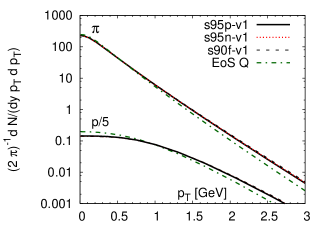
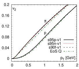
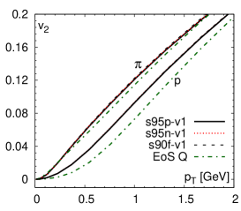
Figure 9: The proton and pion spectra (left) and differential elliptic flow $v_{2}(p_{T})$ of protons and pions (middle and right) in $b=7$fm Au+Au collisions for different EoSs. The results in the left and middle panels are calculated using the same freeze-out temperature $T_{\mathrm{fo}}=125MeV$ for all the EoSs, whereas in the right panel it has been adjusted to produce similar $p_{T}$-distributions. $T_{\mathrm{fo}}=125MeV$ for EoS Q, and $T_{\mathrm{fo}}=140MeV$ for EoSs $s95p\mathrm{-v1}$, $s95n\mathrm{-v1}$ and $s90f\mathrm{-v1}$.

Unfortunately it is not straightforward to calculate the spectra and $v_{2}$ using the various EoSs in the literature discussed earlier. One of the advantages of the Cooper-Frye procedure for freeze-out is that energy, momentum, particle number and entropy are conserved. But, they are conserved only if the equation of state is the same before and after the freeze-out Laszlo , i.e. that the fluid EoS is that of free particles and that the number of degrees of freedom in the fluid is the same than the number of hadrons and resonances which spectrum is calculated. This is not the case with the EoSs discussed here. When calculating the spectra we use the same set of resonances up to 2 GeV mass than what is included in our HRG. Laine and Schroder used resonances up to 2.5 GeV mass, but at, say, $T_{\mathrm{fo}}=125$ MeV freeze-out temperature the difference in energy and entropy is minuscule, about 0.05%. The situation with the other EoSs is more difficult. At the mentioned temperature, the Krakow EoS has 4.5% smaller, EoS L 7% larger, and the HotQCD EoS 22% smaller energy and entropy than hadrons and resonances up to 2 GeV mass. One way to correct this discrepancy is of course to change the number of hadrons and resonances included in the spectra calculation. But, this approach would be tedious since the number of resonances needed to fit the densities in the EoS may depend on temperature. Also there is no telling whether there exists a set of resonances reproducing both densities and pressure at a given temperature, and the number of resonances could be surprisingly small. For example a hadron resonance gas consisting of only pseudo-scalar and vector meson nonets, and baryon octet and decuplet, still has $~{}10$% larger energy density at $T=125$ MeV than HotQCD EoS. Therefore we follow the approach espoused by Csernai Laszlo and Bugaev Bugaev : We require that energy and momentum are conserved locally on the freeze-out surface, i.e.

$$\mathrm{d}\sigma_{\mu}T_{\mathrm{fluid}}^{\mu\nu}=\mathrm{d}\sigma_{\mu}T_{\mathrm{particles}}^{\mu\nu},$$ (19)

where $T_{\mathrm{fluid}}^{\mu\nu}$ is the energy-momentum tensor of the fluid on the surface, and $T_{\mathrm{particles}}^{\mu\nu}$ is the energy-momentum tensor of the emitted particles. To conserve energy and momentum, we allow the temperature and flow velocity of fluid and particles differ, i.e. there is a discontinuity on the surface, and freeze-out is a shock-like phenomenon Bugaev . We have to admit the corrections due to this procedure are small and mostly affect the multiplicity, but consider obeying the conservation laws worth the extra effort.

At first we use the same freeze-out energy density we used when comparing our parametrization to EoS Q, $\epsilon=0.065$ GeV/fm³, for all EoSs. The corresponding temperatures for each EoS are listed in Table 3.

	$\epsilon_{\mathrm{fo}}$	$T_{\mathrm{fluid}}$	$T_{\mathrm{particles}}$	$\epsilon_{\mathrm{fo}}$	$T_{\mathrm{fluid}}$	$T_{\mathrm{particles}}$
$s95p-\mathrm{v1}$	0.065	125	125	0.14	140	140
HotQCD	0.065	129	125	0.11	139	135
Laine	0.065	125	125	0.14	140	140
EoS L	0.065	124	126	0.11	134	136
Krakow	0.065	126	125	0.185	146	145

Table 3: The freeze-out energy densities (in GeV/fm³) and corresponding temperatures (in MeV) for fluid and particles for each EoS used in the calculations shown in Fig. 10

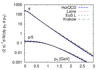
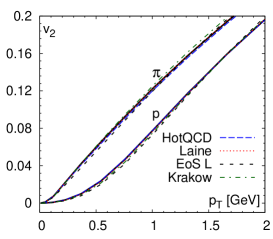
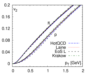
Figure 10: The proton and pion spectra (left) and differential elliptic flow $v_{2}(p_{T})$ of protons and pions (middle and right) in $b=7$fm Au+Au collisions for $s95p\mathrm{-v1}$ (solid black line) and different EoSs in the literature LS ; chojnacki07 ; chojnacki08 ; heinz08 ; hot_eos . The results in the left and middle panels are calculated using the same freeze-out energy density $\epsilon_{\mathrm{fo}}=0.065$ GeV/fm³ for all the EoSs, whereas in the right panel it has been adjusted to produce similar $p_{T}$-distributions, see text and Table 3

In the left panel of Fig. 10 we show the $p_{T}$ distributions of pions and protons in $b=7$ fm Au+Au collision. The differences in distributions are small, and the general behavior is what can be expected based on the stiffness of the EoSs and the flow anisotropy: The Krakow EoS is the stiffest, and leads thus to the flattest spectra. The EoS by Laine and Schröder leads to behavior almost identical to $s95p$-v1, and the HotQCD EoS and EoS L are the softest and have slightly steeper spectra than the other EoSs. For the $p_{T}$-differential anisotropy of pions and protons the systematics is the same than seen for our parametrizations: when the freeze-out criterion is the same for all the EoSs, $v_{2}(p_{T})$ is basically independent of the EoS, as shown in the middle panel of Fig. 10. After the freeze-out criterion is adjusted to reproduce spectra obtained using EoS Q, the pion $v_{2}(p_{T})$ is independent of the EoS, but the proton anisotropy shows some sensitivity, see the right panel of Fig. 10. The differences between the EoSs are small and thus the differences in $v_{2}(p_{T})$ are small, but an ordering according to the stiffness of the EoS is visible: The Krakow EoS is hardest, and its proton $v_{2}(p_{T})$ is largest at small $p_{T}$, whereas the HotQCD EoS and EoS L are softest and lead to lowest $v_{2}(p_{T})$ of protons at low $p_{T}$. After all the main results of this comparison are that the differences in the lattice EoS parametrization in the literature are small and not observable in the $p_{T}$-differential elliptic flow, and that energy conservation at freeze-out is not trivial if the EoS at freeze out is not that of free hadron resonance gas.

Finally we want to compare the results of our calculations with data. Since all of our parametrizations lead to practically identical spectra and $v_{2}$, we use only $s95p$-v1 for simplicity, and compare the results to those obtained using EoS Q in Ref. pasi05 . First we fix all the parameters by requiring the reproduction of pion and net-proton ($p-\bar{p}$) spectra in the 0-5% most central Au+Au collisions at $\sqrt{s_{\mathrm{NN}}}=200$ GeV energy. The resulting spectra are shown in the left panel of Fig. 11, and the freeze-out temperatures are the same than mentioned before, $T_{\mathrm{fo}}=125MeV$ for EoS Q, and $T_{\mathrm{fo}}=140MeV$ for EoSs $s95p-\mathrm{v1}$. Since we assume chemical equilibrium we cannot reproduce both proton and anti-proton yields at such a low temperature. Our parametrization is for zero baryochemical potential, so we cannot calculate net-protons either, but we approximate them by having a finite baryon density in the calculation, and converting this density into a finite chemical potential at freeze-out by using a HRG EoS which allows a finite net baryon density. The right panel of Fig. 11 shows the $p_{T}$-differential elliptic flow of pions and anti-protons in minimum bias Au+Au collisions at the same energy. As earlier, the pion $v_{2}(p_{T})$ is very similar for both EoSs, but the anti-proton $v_{2}(p_{T})$ is quite different. In fact for the realistic EoS the anti-proton $v_{2}$ is largely overpredicted, while we have a reasonable agreement with the data when the bag model EoS Q is used. This is very similar to the finding of Ref. pasi05 . Also the Krakow group seem to overpredict the proton $v_{2}$ chojnacki08 indicating that this could be a general feature of ideal hydrodynamic models using more realistic EoS. The first results indicate that dissipative effects can at least reduce this problem Bozek:2009 .

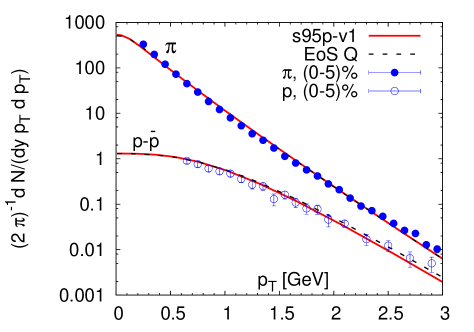
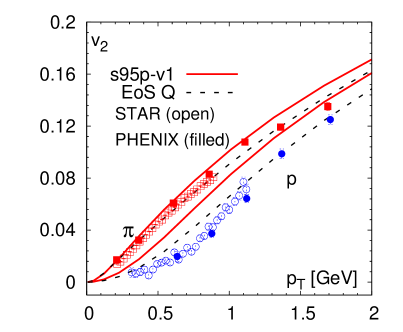
Figure 11: Pion ($\pi^{+}$) and net-proton ($p-\bar{p}$) spectra in 0-5% most central (left), and pion and antiproton $p_{T}$-differential elliptic flow $v_{2}(p_{T})$ in minimum bias (right) Au+Au collisions at $\sqrt{s_{\mathrm{NN}}}=200$ GeV compared with hydrodynamic calculations using two different EoSs and assuming chemical equilibrium. The data was taken by the PHENIX Phenix and the STAR Star collaborations.

This analysis has been repeated assuming partial chemical equilibrium in the hadronic phase. The details of this analysis are given in the appendix C. Our main finding did not change. Using different EoS for the same initial conditions and kinetic freeze-out temperature has little effect on $v_{2}$ but leads to significant differences in the spectra. If the spectra are fitted to reproduce the experimental data by adjusting the initial conditions, the $p_{T}$-differential elliptic flow of anti-protons becomes too large for lattice based EoS, but agrees reasonably well with EoS Q. On the other hand, the $p_{T}$-differential elliptic flow of pions is clearly too large for both EoSs requiring substantial dissipation to reduce it to fit the data.

VI Conclusion

In this paper we addressed the question to what extent the Hadron Resonance Gas (HRG) model can describe the thermodynamic quantities calculated on the lattice. As discussed above this question is very important for implementing a consistent freeze-out prescription or a consistent switch to transport in hydrodynamic or hybrid models, respectively. We have found that lattice data strongly disagree with the HRG model in the low temperature regime. The reason for this disagreement has been identified with large cutoff effects in the lattice calculations. We also showed that taking into account the discretization effects in the hadron spectrum in the HRG model leads to a good agreement with the lattice data. In fact, we find that for some quantities the HRG model works well to unexpectedly high temperatures. Based on this observation we constructed several parametrizations of the equation of state which interpolate between the lattice data at high temperature and the resonance gas in the low temperature region. The central quantity in this analysis was the trace anomaly since it is directly calculated on the lattice and the differences in the proposed parametrizations are found in the temperature region where the trace anomaly reaches its maximal value.

We studied the hydrodynamic evolution using three parametrizations of the EoS that interpolate between HRG EoS and the lattice data and compared the results with the corresponding ones obtained using an EoS with a first order phase transition, the so-called EoS Q, as well as several other parametrizations of the EoS used in the literature. We have analyzed the flow in terms of momentum space anisotropy $\epsilon_{p}$, $p_{T}$-differential elliptic flow $v_{2}(p_{T})$ and proton and pion spectra. The three parametrizations of the EoS proposed in this paper as well the the parametrization by Laine and Schröder LS gave very similar results for all of the above quantities. The effect of using different EoS parametrizations is the most visible in $\epsilon_{p}$. The difference in the results obtained with EoS Q and other parametrizations is especially large. Quite surprisingly $v_{2}(p_{T})$ is not sensitive to the choice of the EoS if the same freeze-out temperature is used. The particle spectra on the other hand are sensitive to the EoS. However, the change in the EoS can be compensated by change of the freeze-out temperature. If the freeze-out temperature is adjusted to reproduce the particle spectra we see large differences in the proton $v_{2}(p_{T})$ for EoS Q and other EoS parametrizations. However, for all the other parametrizations considered here, the proton $v_{2}(p_{T})$ is quite similar.

The work presented in this paper should be extended in number of different ways. First we should extend the comparison of lattice QCD results with modified HRG to other fluctuations, including electric charge fluctuations as well as fourth and higher order fluctuations of baryon number, strangeness and electric charge. However, since these quantities were studied in detail only for the p4 action, in the analysis additional assumptions about the cutoff effects in the hadron spectrum have to be made. Furthermore, it would be interesting to study the quark mass effects in the HRG model, especially since recent lattice calculations of the EoS extend to physical values of the light quark masses p4_new_eos . We also should consider the effect of finite baryon potential on the EoS. This will become important for application of hydrodynamic models to heavy ion collisions at lower energies, especially to the proposed RHIC energy scan. Finally, it will be interesting to study the effect of the EoS in the framework of viscous hydrodynamics. We plan to address these issues in forthcoming publications.

Appendix A Hadron masses on the lattice

In this appendix we are going to discuss the cutoff and quark mass dependence of hadron masses calculated on the lattice and give the parameters entering Eqs. (8)-(12). We have fitted the quark (pion) mass and lattice spacing dependence of the $\rho,~{}K^{*},~{}\phi,~{}N$ and $\Omega$ masses obtained in Refs. bazavov09 ; bernard07 ; bernard04 ; bernard01 by a simple Ansatz

$$r_{1}m=r_{1}m_{0}+\frac{a_{1}(r_{1}m_{\pi})^{2}}{1+a_{2}x}+\frac{b_{1}x}{1+b_{2}x},~{}x=(a/r_{1})^{2}$$ (20)

The values of the fit parameters $m_{0}$, $a_{1},~{}a_{2},~{}b_{1}$ and $b_{2}$ are given in Table 4. In Figs. 12, 13 and 14 we show the above parametrization against the available lattice data. Here we note that the lattice data for the $\Omega$ mass have been corrected to take into account that the physical strange quark mass is slightly smaller that the one used in lattice simulations. It turns out that Eq. (20) reproduces the experimental values of the hadron masses in continuum limit at the physical point $r_{1}m_{\pi}=0.226$. This justifies the use of Eqs. (8)-(12) for the evaluation of the hadron masses in the HRG model.

As discussed in the main text due to lack of detailed lattice studies we used Eq. (8) and Eqs. (10)-(12) to evaluate the mass of the $\Delta$ resonance as well as single and double strange baryons with values of the parameters in Table 4 corresponding to the nucleon. In Figure 15 we compare our estimates of the $\Delta$, $\Lambda$ and $\Xi$ baryon masses shown as lines with available lattice data from the MILC collaboration bernard04 ; bernard01 .

	$r_{1}m_{0}$	$a_{1}$	$b_{1}$	$a_{2}$	$b_{2}$
$\rho$	1.17856	0.496745	2.03538	0.958366	6.39177
$K^{*}$	1.41505	0.228217	2.07898	0	0
$\phi$	1.60476	0.056901	2.74519	0	0
$N$	1.51418	0.933405	1.65138	1.27391	1.65138
$\Omega$	2.66589	0.056779	1.74275	0	0

Table 4: The values of the parameters appearing in Eq. (20) for different hadrons.

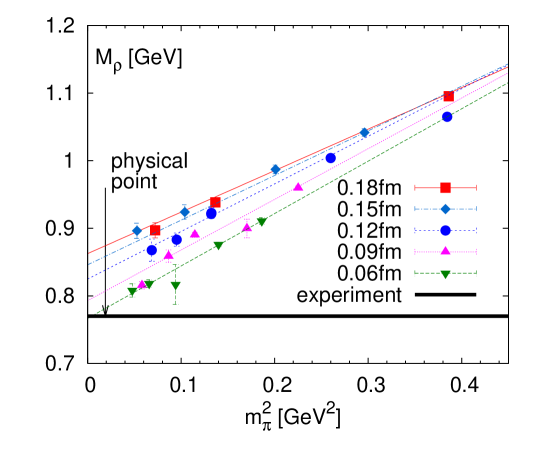
Figure 12: The $\rho$-meson (right) masses calculated on the lattice using asqtad action bernard01 ; bernard04 ; milc_unpub and compared with Eq. (20) (lines).

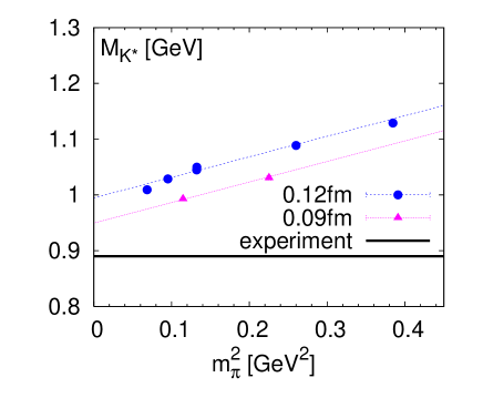
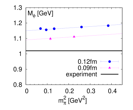
Figure 13: The $K^{*}$ (left) and $\phi$-meson (right) masses calculated on the lattice using asqtad action bernard01 ; bernard04 and compared with Eq. (20) (lines).

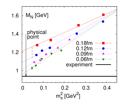
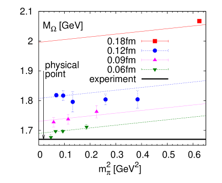
Figure 14: The nucleon mass bernard01 ; bernard04 ; milc_unpub (left) and the $\Omega$ baryon mass bazavov09 (right) calculated with asqtad action and compared with our parametrization.

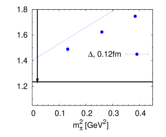
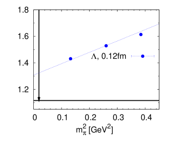
Figure 15: The baryon masses calculated for asqtad action bernard01 ; bernard04 ; milc_unpub and compared with our parametrization.

Appendix B Fitting procedure

Here we describe in detail how we fit the trace anomaly of lattice and hadron resonance gas. The two first terms of the inverse polynomial Ansatz (Eq. 15)

$$(e-3P)/T^{4}=d_{2}/T^{2}+d_{4}/T^{4}+c_{1}/T^{n_{1}}+c_{2}/T^{n_{2}}$$ (21)

appear to provide good fit of the lattice data at high temperatures, $T>250$ MeV hot_eos . We want to join this parametrization to the trace anomaly of hadron resonance gas and require that the trace anomaly and its first and second derivative with respect to temperature are continuous where joined. Thus, we need one additional term with negative coefficient $c_{1}$ and exponent $n_{1}>4$ to produce a peak around $T\approx 200$ MeV, and another with positive coefficient $c_{2}$ and exponent $n_{2}>n_{1}$ to make the second derivative continuous. We calculate the trace anomaly of hadron resonance gas using all the resonances up to 2 GeV mass in the summary of the 2004 edition of the Review of Particle Physics PDG2004 . We note that including all the resonances up to $2.5$GeV instead of $2$GeV mass gives result for the trace anomaly, which is only $2\%$ larger at $T=170$MeV and $3\%$ larger at $T=180$MeV. This change is definitely smaller than the expected discrepancies between HRG and lattice at these temperatures.

In the ansatz we have seven unknown parameters: the coefficients $d_{2}$, $d_{4}$, $c_{1}$ and $c_{2}$, exponents $n_{1}$ and $n_{2}$, and the switching temperature $T_{0}$. We have four constraints, the continuity of the trace anomaly and its derivatives at $T_{0}$, and the requirement $s(T=800\,\mathrm{MeV})=0.95\cdot s_{\mathrm{SB}}$ or $s(T=800\,\mathrm{MeV})=0.90\cdot s_{\mathrm{SB}}$. The requirement of the continuity of the derivatives gives two equations to fix the parameters $c_{1}$ and $c_{2}$:

$$c_{2} = \frac{2(n_{1}-2)}{n_{2}(n_{2}-n_{1})}T^{n_{2}-2}d_{2}+\frac{4(n_{1}-4)}{n_{2}(n_{2}-n_{1})}T^{n_{2}-4}d_{4}$$

$$+ \frac{n_{1}+1}{n_{2}(n_{2}-n_{1})}T^{n_{2}+1}G_{1}(T_{0})+\frac{1}{n_{2}(n_{2}-n_{1})}T^{n_{2}+2}G_{2}(T_{0})$$

$$c_{1} = \frac{2(n_{2}-2)}{n_{1}(n_{1}-n_{2})}T^{n_{1}-2}d_{2}+\frac{4(n_{2}-4)}{n_{1}(n_{1}-n_{2})}T^{n_{1}-4}d_{4}$$

$$+ \frac{n_{2}+1}{n_{1}(n_{1}-n_{2})}T^{n_{1}+1}G_{1}(T_{0})+\frac{1}{n_{1}(n_{1}-n_{2})}T^{n_{1}+2}G_{2}(T_{0}),$$

where

$$\left.\frac{d}{dT}\frac{\epsilon-3P}{T^{4}}\right|_{HG}\equiv G_{1}(T)\qquad\mathrm{and}\qquad\left.\frac{d^{2}}{dT^{2}}\frac{\epsilon-3P}{T^{4}}\right|_{HG}\equiv G_{2}(T).$$

From Eq.(14) and $Ts=\epsilon+P$ we obtain

$$\frac{s}{T^{3}}=d_{2}\left(\frac{2}{T_{0}^{2}}-\frac{1}{T^{2}}\right)+\frac{d_{4}}{T_{0}^{4}}+\frac{c_{1}}{n_{1}}\left(\frac{4}{T_{0}^{n_{1}}}+\frac{n_{1}-4}{T^{n_{1}}}\right)+\frac{c_{2}}{n_{2}}\left(\frac{4}{T_{0}^{n_{2}}}+\frac{n_{2}-4}{T^{n_{2}}}\right)+\frac{4P(T_{0})}{T_{0}^{4}}.$$ (22)

Since entropy at $T=800$ MeV is fixed, we can use the above equation to constrain $d_{4}$,

$$d_{4}=d_{4}(d_{2},n_{1},n_{2},T_{0}).$$ (23)

We can thus express the parameters $c_{1}$, $c_{2}$ and $d_{4}$ in terms of $d_{2}$, $n_{1}$, $n_{2}$ and $T_{0}$, and use the continuity of the trace anomaly to fix $T_{0}$. We get an equation

$$\left.\frac{\epsilon-3P}{T^{4}}\right|_{HG}(T_{0})=\frac{d_{2}}{T_{0}^{2}}+\frac{d_{4}(d_{2},n_{1},n_{2},T_{0})}{T_{0}^{4}}+\frac{c_{1}(d_{2},n_{1},n_{2},T_{0})}{T_{0}^{n_{1}}}+\frac{c_{2}(d_{2},n_{1},n_{2},T_{0})}{T_{0}^{n_{2}}},$$ (24)

which can be evaluated numerically to obtain $T_{0}$. This procedure leaves us with three unknowns $d_{2}$, $n_{1}$ and $n_{2}$, which are chosen to fit the lattice data. However, such a fitting procedure would be highly nonlinear. We simplify the problem by requiring that the exponents are integers, and use brute force: We make a single parameter ($d_{2}$) fit with all the integer values $4<n_{1}<31$, and $n_{1}<n_{2}<43$, and choose the values $n_{1}$ and $n_{2}$ which lead to the smallest $\chi^{2}$. Alternatively we can fix $T_{0}$ to a prescribed value, use Eq. (24) to fix the value of $d_{2}$, and use only $n_{1}$ and $n_{2}$ to perform the fit.

In our fit we use the lattice data for $T>250$ MeV obtained with p4 action on $N_{\tau}=8$ lattices as they extend to sufficiently high temperature hot_eos . In addition, we include $N_{\tau}=6$ p4 data for $T>500$MeV p4_eos . The fits in general do not reproduce the lattice data in peak region ($190{\rm MeV}<T<250{\rm MeV}$). On the other hand the height of the peak in the trace anomaly may be affected by discretization effects. This can be seen as a difference between the $N_{\tau}=6$ and $N_{\tau}=8$ results. Assuming that discretization effects in the peak height go like $1/N_{\tau}^{2}$ we can estimate the trace anomaly at $T=206$MeV to be $5.7\pm 0.15$. We can use this value as an additional data point in our fits. We label different parametrization of the trace anomaly obtained using different constraints on the entropy density at $T=800$MeV and its height in the temperature region $190{\rm MeV}<T<250{\rm MeV}$ as $s95p\mathrm{-v1}$, $s95n\mathrm{-v1}$, $s90f\mathrm{-v1}$ etc. The first three characters stand for the constrain on the entropy density (90% or 95% of the ideal gas value). The fourth character stands for additional constraints on the trace anomaly in the peak region. Namely, “n” stands for a fit with no constraints: using data for $T>250$ MeV, and $T_{0}$ as a free parameter in the fit. “p” means having an additional data point of $5.7\pm 0.15$ at $T=206$ MeV to constrain the peak, and “f” stands for a fixed value $T_{0}=170$ MeV in the fit. Finally “v1” is the version number of the current parametrization. The value of the parameters $d_{2}$, $d_{4}$, $c_{1}$, $c_{2}$, $n_{1}$, $n_{2}$ and $T_{0}$ for different fits are given in Table 2. This procedure was designed for numerical applications when the trace anomaly is numerically evaluated using Eq.(1) and laws of thermodynamics. For practical purposes we also provide a parametrized version of the trace anomaly of the hadronic part of our EoS. We choose a polynomial

$$\frac{\epsilon-3P}{T^{4}}=a_{1}T^{l_{1}}+a_{2}T^{l_{2}}+a_{3}T^{l_{3}}+a_{4}T^{l_{4}}$$ (25)

and fit it to the trace anomaly of the hadron resonance gas evaluated in the temperature interval $70<T/\mathrm{MeV}<190$ with 1 MeV steps assuming that each point has equal “error”. The limits have entirely utilitarian origin: in hydrodynamical applications the system decouples well above 70 MeV temperature and only a rough approximation of the EoS, $P=P(\epsilon)$, is needed at lower temperatures. On the other hand we expect to switch to the lattice parametrization below 190 MeV, and the HRG EoS above that is not needed either. We fix the exponents in Eq.(25) again using brute force. We require them to be integers, go through all the combinations $0\leq l_{1}<l_{2}<l_{3}<l_{4}\leq 10$, fit the parameters $a_{1}$, $a_{2}$, $a_{3}$, $a_{4}$ to the HRG trace anomaly evaluated with 1 MeV intervals, and choose the values $l_{1},~{}l_{2},~{}l_{3}$ and $l_{4}$ which minimize the $\chi^{2}$. We end up with $l_{1}=1$, $l_{2}=3$, $l_{3}=4$, $l_{4}=10$, and $a_{1}=4.654$ GeV^-1, $a_{2}=-879$ GeV^-3, $a_{3}=8081$ GeV^-4, $a_{4}=-7039000$ GeV^-10 . To obtain the EoS, one also needs the pressure at the lower limit of the integration (see Eq.(14)) $T_{\mathrm{low}}=0.07$ GeV: $P(T_{\mathrm{low}})/T^{4}_{\mathrm{low}}=0.1661$. Our EoSs are also available in a tabulated form at wiki .

Appendix C Spectra and elliptic flow for partial chemical equilibrium

In this appendix we discuss the elliptic flow and the spectra of protons and pions and their sensitivity on EoS when partial chemical equilibrium Bebie:1991 ; hirano_pce ; pasi07 is assumed to reproduce the observed particle yields. The EoS for the system in partial chemical equilibrium is available in tabulated form [62]. We again calculate the flow in Au+Au collision at $\sqrt{s_{\mathrm{NN}}}=200$ GeV with impact parameter $b=7$ fm. First we used the same initial condition and the same freeze-out temperature for all EoSs, namely $T_{\mathrm{chem}}=150$MeV for the chemical freeze-out temperature and $T_{\mathrm{kin}}=120$MeV for the kinetic freeze-out temperature. The initial time for the hydrodynamic evolution was chosen to be $\tau=0.6$fm and the initial entropy density was chosen as for the case of chemical equilibrium. The results are shown in Figure 16. As one can see the elliptic flow is not very sensitive to the choice of EoS if everything else is kept unchanged, and all three parametrizations used in the analysis give almost the same result. The spectra are much more sensitive to the EoS but again there is no difference for the different lattice parametrizations.

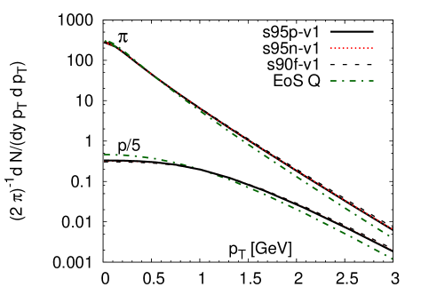
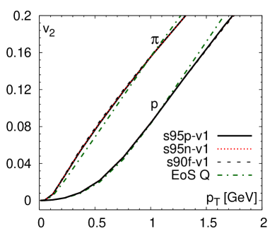
Figure 16: The $p_{T}$-differential elliptic flow $v_{2}(p_{T})$ of protons and pions (left) and proton and pion spectra (right) for different EoSs in $b=7$ fm Au+Au collision when chemical freeze-out takes place at $T_{\mathrm{chem}}=150$ MeV and kinetic at $T_{\mathrm{kin}}=120$ MeV.

For a proper discussion on the sensitivity of elliptic flow on the EoS, one has to again re-tune the calculation to reproduce the experimental results on the $p_{T}$-spectra. We obtained the best results by keeping the chemical and kinetic freeze-out temperatures, $T_{\mathrm{chem}}=150$MeV and $T_{\mathrm{kin}}=120$MeV unchanged, and tuned the initial conditions. For EoS Q we used $\tau_{0}=0.2$fm and initial entropy density which scales with the number of binary collisions (see Ref. pasi07 ). For the $s95p$-v1 parametrization of the EoS we used two different initial conditions. One with $\tau_{0}=0.8$fm and initial entropy density proportional to the number of binary collisions, and a second one with $\tau_{0}=0.2$fm and initial entropy density scaling with a combination of binary collisions and number of participants. The corresponding results are shown in Figure 17. We see again that the lattice based EoS give larger $p_{T}$-differential elliptic flow for the protons than EoS Q for both initial conditions. In this case, however, the EoS Q does not do a good job of describing the data either, in agreement with previous findings hirano_pce ; pasi07 . Especially the pion $p_{T}$-differential $v_{2}$ is too large for all EoSs, and there is clearly room for significant dissipation to reduce the anisotropy. It is also worth to notice that the uncertainty related to the initial state is at least as large as the effect of the EoS on the proton $v_{2}(p_{T})$ and better theoretical constraints to the initial state are needed.

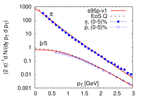
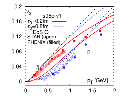
Figure 17: Pion ($\pi^{+}$) and net-proton ($p-\bar{p}$) spectra in 0-5% most central (left), and pion and anti-proton $p_{T}$-differential elliptic flow $v_{2}(p_{T})$ in minimum bias Au+Au collisions at $\sqrt{s_{\mathrm{NN}}}=200$ GeV compared with hydrodynamic calculations using two different EoSs and assuming chemical freeze-out at $T_{\mathrm{chem}}=150$MeV. The calculation using EoS s95p-v1 was done using two different initial states, see the text. The data was taken by the PHENIX Phenix and the STAR Star collaborations.

References

- (1) M. Hindmarsh and O. Philipsen, Phys. Rev. D 71, 087302 (2005) [arXiv:hep-ph/0501232].
- (2) M. Laine, PoS LAT2006, 014 (2006) [arXiv:hep-lat/0612023].
- (3) P. F. Kolb and U. W. Heinz, arXiv:nucl-th/0305084. P. Huovinen, arXiv:nucl-th/0305064.
- (4) Y. Aoki, G. Endrodi, Z. Fodor, S. D. Katz and K. K. Szabo, Nature 443, 675 (2006) [arXiv:hep-lat/0611014].
- (5) P. Huovinen, Nucl. Phys. A 761, 296 (2005) [arXiv:nucl-th/0505036].
- (6) P. Petreczky, Nucl. Phys. Proc. Suppl. 140, 78 (2005) [arXiv:hep-lat/0409139].
- (7) C. DeTar, PoS LAT2008, 001 (2008) [arXiv:0811.2429 [hep-lat]].
- (8) C. Bernard et al., Phys. Rev. D 75, 094505 (2007) [arXiv:hep-lat/0611031].
- (9) M. Cheng et al., Phys. Rev. D 77, 014511 (2008) [arXiv:0710.0354 [hep-lat]].
- (10) A. Andronic, P. Braun-Munzinger, K. Redlich and J. Stachel, Phys. Lett. B 571, 36 (2003) [arXiv:nucl-th/0303036].
- (11) J. Noronha-Hostler, J. Noronha and C. Greiner, Phys. Rev. Lett. 103, 172302 (2009) [arXiv:0811.1571 [nucl-th]].
- (12) P. Braun-Munzinger, J. Stachel and C. Wetterich, Phys. Lett. B 596, 61 (2004) [arXiv:nucl-th/0311005].
- (13) F. Karsch, K. Redlich and A. Tawfik, Eur. Phys. J. C 29, 549 (2003) [arXiv:hep-ph/0303108].
- (14) F. Karsch, K. Redlich and A. Tawfik, Phys. Lett. B 571, 67 (2003) [arXiv:hep-ph/0306208].
- (15) S. Ejiri, F. Karsch and K. Redlich, Phys. Lett. B 633, 275 (2006) [arXiv:hep-ph/0509051].
- (16) M. Cheng et al., Phys. Rev. D 79, 074505 (2009) [arXiv:0811.1006 [hep-lat]].
- (17) P. Gerber and H. Leutwyler, Nucl. Phys. B 321, 387 (1989).
- (18) R. Dashen, S. Ma and H.J. Berstein, Phys. Rev. 187, 349 (1969).
- (19) R. Venugopalan and M. Prakash, Nucl. Phys. A 546 (1992) 718.
- (20) R. Hagedorn, in Quark Matter ’84, Lecture Notes in Physics, Vol. 211 (Springer, Berlin 1985); R. Hagedorn, Riv. Nuovo Cim. 6, 1 (1983); R. Fiore, R. Hagedorn and F. D’Isep Nuovo Cim. 88 A, 301 (1985).
- (21) L. M. Satarov, M. N. Dmitriev and I. N. Mishustin, Phys. Atom. Nucl. 72, 1390 (2009) [arXiv:0901.1430 [hep-ph]].
- (22) F. Cooper and G. Frye, Phys. Rev. D 10, 186 (1974).
- (23) C. Anderlik et al., Phys. Rev. C 59, 3309 (1999) [arXiv:nucl-th/9806004].
- (24) A. Bazavov et al., Phys. Rev. D 80, 014504 (2009) [arXiv:0903.4379 [hep-lat]].
- (25) A. Bazavov et al., arXiv:0903.3598 [hep-lat].
- (26) C. Bernard et al. [MILC Collaboration], PoS LAT2007, 137 (2007) [arXiv:0711.0021 [hep-lat]].
- (27) C. Aubin et al., Phys. Rev. D 70, 094505 (2004) [arXiv:hep-lat/0402030].
- (28) C. W. Bernard et al., Phys. Rev. D 64, 054506 (2001) [arXiv:hep-lat/0104002].
- (29) S. Durr et al., Science 322, 1224 (2008).
- (30) S. Durr et al., Phys. Rev. D 79, 014501 (2009) [arXiv:0802.2706 [hep-lat]].
- (31) C. Bernard, M. Golterman, Y. Shamir and S. R. Sharpe, Phys. Rev. D 77, 114504 (2008) [arXiv:0711.0696 [hep-lat]].
- (32) M. Creutz, PoS LAT2007, 007 (2007) [arXiv:0708.1295 [hep-lat]].
- (33) A. S. Kronfeld, PoS LAT2007, 016 (2007) [arXiv:0711.0699 [hep-lat]].
- (34) M. F. L. Golterman, Nucl. Phys. B 273, 663 (1986); Nucl. Phys. B 278, 417 (1986)
- (35) H. Kluberg-Stern, A. Morel, O. Napoly and B. Petersson, Nucl. Phys. B 220, 447 (1983).
- (36) Y. Aoki, Z. Fodor, S. D. Katz and K. K. Szabó, Phys. Lett. B 643, 46 (2006) [arXiv:hep-lat/0609068]; Y. Aoki, S. Borsányi, S. Durr, Z. Fodor, S. D. Katz, S. Krieg and K. K. Szabó, JHEP 0906, 088 (2009) [arXiv:0903.4155 [hep-lat]].
- (37) Baryon and vector meson masses for fm and fm were calculated by the MILC collaboration but not published
- (38) C. Bernard et al. [MILC Collaboration], Phys. Rev. D 71, 034504 (2005) [arXiv:hep-lat/0405029].
- (39) S. Basak et al. [The MILC Collaboration], PoS LATTICE2008, 175 (2008) [arXiv:0910.0276 [hep-lat]].
- (40) G. Boyd, J. Engels, F. Karsch, E. Laermann, C. Legeland, M. Lutgemeier and B. Petersson, Nucl. Phys. B 469, 419 (1996) [arXiv:hep-lat/9602007].
- (41) P. Petreczky, Nucl. Phys. A 830, 11C (2009) [arXiv:0908.1917 [hep-ph]].
- (42) J. P. Blaizot, E. Iancu and A. Rebhan, Phys. Rev. Lett. 83 (1999) 2906 [arXiv:hep-ph/9906340]; J. P. Blaizot, E. Iancu and A. Rebhan, Phys. Lett. B 523 (2001) 143; [arXiv:hep-ph/0110369]; J. O. Andersen, E. Braaten and M. Strickland, Phys. Rev. Lett. 83 (1999) 2139 [arXiv:hep-ph/9902327]; J. O. Andersen, M. Strickland and N. Su, arXiv:0911.0676 [hep-ph].
- (43) P. F. Kolb, J. Sollfrank and U. W. Heinz, Phys. Rev. C 62, 054909 (2000) [arXiv:hep-ph/0006129].
- (44) P. Huovinen, Eur. Phys. J. A 37, 121 (2008) [arXiv:0710.4379 [nucl-th]].
- (45) M. Chojnacki and W. Florkowski, Acta Phys. Polon. B 38, 3249 (2007) [arXiv:nucl-th/0702030].
- (46) M. Chojnacki, W. Florkowski, W. Broniowski and A. Kisiel, Phys. Rev. C 78, 014905 (2008) [arXiv:0712.0947 [nucl-th]].
- (47) M. Laine and Y. Schroder, Phys. Rev. D 73, 085009 (2006) [arXiv:hep-ph/0603048].
- (48) K. Kajantie, M. Laine, K. Rummukainen and Y. Schroder, Phys. Rev. Lett. 86, 10 (2001) [arXiv:hep-ph/0007109]; K. Kajantie, M. Laine, K. Rummukainen and M. E. Shaposhnikov, Nucl. Phys. B 503, 357 (1997) [arXiv:hep-ph/9704416].
- (49) P. Romatschke and U. Romatschke, Phys. Rev. Lett. 99, 172301 (2007) [arXiv:0706.1522 [nucl-th]]; M. Luzum and P. Romatschke, Phys. Rev. C 78, 034915 (2008) [Erratum-ibid. C 79, 039903 (2009)] [arXiv:0804.4015 [nucl-th]].
- (50) H. Song and U. W. Heinz, Phys. Rev. C 78, 024902 (2008) [arXiv:0805.1756 [nucl-th]].
- (51) Y. Aoki, Z. Fodor, S. D. Katz and K. K. Szabó, JHEP 0601, 089 (2006) [arXiv:hep-lat/0510084].
- (52) P. Petreczky, Nucl. Phys. A 785, 10 (2007) [arXiv:hep-lat/0609040].
- (53) T. S. Biro and J. Zimányi, Phys. Lett. B 650, 193 (2007) [arXiv:hep-ph/0607079].
- (54) M. Chojnacki, personal communication.
-
(55)
S. Katz, Plenary talk presented at Quark Matter 2005,
http://qm2005.kfki.hu/Talks/Globe/aug5/0930//0930_Katz.pdf - (56) P. Huovinen, P. F. Kolb, U. W. Heinz, P. V. Ruuskanen and S. A. Voloshin, Phys. Lett. B 503, 58 (2001) [arXiv:hep-ph/0101136].
- (57) K. A. Bugaev, M. I. Gorenstein and W. Greiner, J. Phys. G 25, 2147 (1999) [arXiv:nucl-th/9906088].
- (58) S. S. Adler et al. [PHENIX Collaboration], Phys. Rev. C 69 (2004) 034909 [arXiv:nucl-ex/0307022]; S. S. Adler et al. [PHENIX Collaboration], Phys. Rev. Lett. 91 (2003) 182301 [arXiv:nucl-ex/0305013].
- (59) J. Adams et al. [STAR Collaboration], Phys. Rev. C 72, 014904 (2005) [arXiv:nucl-ex/0409033].
-
(60)
P. Bozek,
arXiv:0911.2397 [nucl-th];
H. Song, Ph.D. Thesis, Ohio State University, 2009 [arXiv:0908.3656 [nucl-th]]. - (61) M. Cheng et al., arXiv:0911.2215 [hep-lat].
- (62) https://wiki.bnl.gov/hhic/index.php/Lattice_calculatons_of_Equation_of_State and https://wiki.bnl.gov/TECHQM/index.php/Bulk_Evolution.
- (63) S. Eidelman et al. [Particle Data Group], Phys. Lett. B 592, 1 (2004).
- (64) H. Bebie, P. Gerber, J. L. Goity and H. Leutwyler, Nucl. Phys. B 378, 95 (1992).
- (65) T. Hirano and K. Tsuda, Phys. Rev. C 66, 054905 (2002) [arXiv:nucl-th/0205043].