Abstract

The evolutionary dynamics of HIV during the chronic phase of infection is driven by the host immune response and by selective pressures exerted through drug treatment. To understand and model the evolution of HIV quantitatively, the parameters governing genetic diversification and the strength of selection need to be known. While mutation rates can be measured in single replication cycles, the relevant effective recombination rate depends on the probability of coinfection of a cell with more than one virus and can only be inferred from population data. However, most population genetic estimators for recombination rates assume absence of selection and are hence of limited applicability to HIV, since positive and purifying selection are important in HIV evolution. Yet, little is known about the distribution of selection differentials between individual viruses and the impact of single polymorphisms on viral fitness.

Here, we estimate the rate of recombination and the distribution of selection coefficients from time-resolved sequence data tracking the evolution of HIV within single patients. By examining temporal changes in the genetic composition of the population, we estimate the effective recombination to be $\rho=1.4\pm 0.6\times 10^{-5}$ recombinations per site and generation. Furthermore, we provide evidence that for at least 15% of the non-synonymous polymorphisms observed, selection coefficients exceed $0.8$% per generation.

These results provide a basis for a more detailed understanding of the evolution of HIV. A particularly interesting case is evolution in response to drug treatment, where recombination can facilitate the rapid acquisition of multiple resistance mutations. With the methods developed here, more precise and more detailed studies will be possible, as soon as data with higher time resolution and greater sample sizes is available.

Author Summary

Evolution, in viruses and other organisms, is the result of random genetic diversification by mutation and recombination, selection as well as the stochastic nature of replication and death. For most organisms, these evolutionary forces have to be estimated from static snapshots of the population. This inference requires models of the population dynamics that typically assume that some of the evolutionary forces can be neglected. In rapidly and vigorously evolving organisms like HIV, such assumptions are questionable. As opposed to most other cases, however, time resolved data is available for HIV. We present a direct estimation of the recombination rate and selection coefficients in the intrapatient dynamics of HIV using time resolved data. We find that the effective recombination rate in HIV is similar to the substitution rate at $\rho=1.4\pm 0.6\times 10^{-5}$ per generation and site, rather than much larger as previously reported. Furthermore, we study the distribution of selection coefficients and find that a significant fraction (15%) of the observed non-synonymous polymorphisms in the env are selected for with coefficients ranging from $0.8$% to 2% per generation. Currently, the estimation is limited by the scarceness of the available data, but much more detailed and accurate studies will be possible in the near future.

Introduction

The human immunodeficiency virus (HIV-1) ranks among the most rapidly evolving entities known [1], enabling the virus to continually escape the immune system. After infection with HIV, patients typically enter an asymptomatic period lasting several years during which the virus is present at low to medium levels, typically at a viral load of $<50$ to $10^{4}$ copies per ml plasma. Nevertheless, the number of virions produced and removed is estimated to be around $10^{10}$ per day with a generation time slightly less than two days [2]. Due to this rapid turnover and the high mutation rate of $2.5\times 10^{-5}$ per site and generation, the sequence diversity of HIV within a single patient can rise to $\approx 5$% (env gene) within a few years and the divergence from the founder strain increases by $\approx 1$% per year [3], although this rate is not constant [4]. The genotypic diversity is subject to positive selection for novel variants that are not recognized by the host immune system or that reduce the sensitivity to anti-retroviral drugs [5, 6, 7], as well as to purifying selection by functional constraints [8]. In addition to high substitution rates and strong selection, genomes of different HIV particles within the same host frequently exchange genetic information. This form of viral recombination works as follows: Whenever a cell is coinfected by two or more viruses, the daughter virions can contain two RNA strands from different viruses[9, 10]. In the next round of infection, recombinant genomes are generated by template switching of the retrotranscriptase while producing cDNA. It has been shown that recombination in HIV contributes significantly to the genetic diversity within a patient [11, 12, 13]. In cases of super-infection with several HIV-1 subtypes, recombination can give rise to novel forms that become part of the global epidemic [14].

The observation of recombinant viruses after a change in anti-retroviral drug therapy [15] suggests that recombination might play an important role in the evolution of drug resistance, as predicted by theoretical models [16]. The amount by which recombination speeds up the evolution of drug resistance depends on the parameters governing the population dynamics [17], many of which are not known to sufficient accuracy. In vitro estimates of the recombination rate have shown that the retrotranscriptase switches templates about $2-3$ times while transcribing the entire genome, resulting in a recombination rate of $3\times 10^{-4}$ per site and generation [18, 19]. However, the bare template switching rate is only of secondary importance, since recombination can generate diversity only if the virion contains two RNA strands that originate from different viruses, which requires coinfection of host cells[20]. The effective in vivo recombination rate is therefore a compound quantity, to which the template switching rate and the probability of coinfection of a single host cell contribute. This effective recombination rate has been estimated with coalescent based methods developed in population genetics [21, 13]. These methods use a single sample of sequences obtained from the diverse population and estimate the recombination rate from topological incongruencies in the phylogenetic tree of the sequence sample. Together with an estimate of the mutation rate, this allows to estimate the recombination rate in real time units. Shriner et al. [13] report an estimate of $1.38\times 10^{-4}$ per site and generation, implying almost ubiquitous coinfection of host cells.

Here, we present a different method to estimate recombination rates from longitudinal sequence data, which has been obtained from 11 patients at approximately 6 month intervals [22, 3]. By comparing sequence samples from successive time points, we can estimate recombination rates from the distance and time dependence of the probability of cross-over between pairs of polymorphic sites. We find that the effective rate of recombination is $\rho\approx 1.4\times 10^{-5}$ per site and generation. Furthermore, we estimate the strength of selection on nonsynonymous polymorphisms by measuring the rate at which allele frequencies change. We find that a fraction of about 15% of the observed nonsynonymous polymorphisms are selected stronger than $0.8$%  per generation.

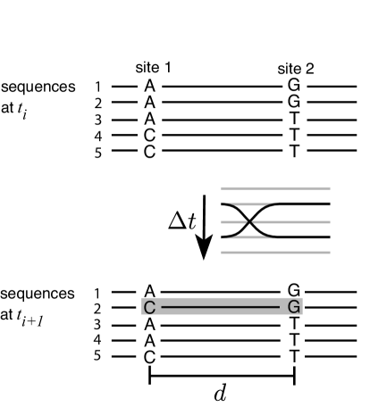
Figure 1: Recombination produces new haplotypes. At time point $t_{i}$, a pair of polymorphic sites is observed in three different combinations A…G, A…T, and C…T. Recombination can generate the missing haplotype C…G (grey box) from one time point to the next with a rate proportional to the product of the distance $d$ between the two sites and the time interval $\Delta t$ between the two observations. Since no other process depends on this combination of parameters, we can estimate the recombination rate using this dependence.

Results

Time resolved sequence data of the C2-V5 region of the env gene was available from eleven patients over a time-span of 6-13 years with sequence samples taken typically every 6-10 month [3, 23]. At each time point, about 5-20 viruses had been sequenced successfully. These sequences were aligned as described in Methods. We will use the temporal variation in genetic diversity to estimate the recombination rate and selection coefficients that govern the dynamics of the viral population.

Recombination rate

Recombination produces new combinations of alleles from existing genetic variation and randomizes the distribution of genotypes. To illustrate this process and the challenges of estimating recombination rates, consider the pair of polymorphic sites in Figure 1. Generically such a pair will have arisen by the following sequence of events: (i) Site 1 becomes polymorphic by mutation, e.g. A/C. (ii) A mutation occurs at site 2 on a genome that carries one of the variants of site 1, e.g. giving rise to the haplotypes A…T, A…G and C…T. (iii) The missing haplotype, e.g. C…G, can be generated by further mutation (A$\to$C at site 1 or T$\to$G at site 2) or by crossing over two of the existing haplotypes, as illustrated in Figure 1. In population genetics, the occurrence of the fourth haplotype is often taken as sufficient condition for recombination (the four gamete test[24]). While this is true for bacteria and eukaryotes because of their low mutation rates, the HIV population within a patient is large and mutates rapidly [25]. Hence, the biggest challenge in estimating recombination rates is to separate recombination from recurrent mutations or homoplasy. A second confounding effect stems from the small number of sequences available per time point, such that the sequences containing the fourth haplotype could have been missed due to undersampling. To disentangle these two effects from recombination, we make use of the fact that only the recombination rate depends strongly on the distance between the two sites, while recurrent mutations and sampling noise should not.

For each pair of biallic sites at time $t_{i}$ that was found in three of the four possible haplotypes, we asked whether the missing haplotype is observed the at time $t_{i+1}$ (comp. figure 1) and calculated the frequency of this event as a function of the separation of the two sites, as shown in figure 2A. This frequency increases with the separation of the two sites from about 0.1 to about 0.35 at 500 bp separation, in line with the expectation that recombination is more rapid between distant sites. To corroborate that this distance dependence is indeed due to recombination, we performed the following similar analysis: The curve labelled “other haplotypes” in figure 2A shows the frequency of observing a haplotype at time $t_{i+1}$, which contains alleles not present at time $t_{i}$ again averaged over all available data. Any such haplotype could have arisen by mutation in the time interval between $t_{i}$ and $t_{i+1}$, or could have been present at time $t_{i}$ but not sampled. It cannot, however, be assembled by recombination from the alleles found at time $t_{i}$. The important observation is that the frequency of observing such a haplotype does not increase with distance. This is consistent with our expectation that an additional mutation or undersampling should be independent of an additional polymorphism nearby. The clear separation between the two classes of haplotypes suggests that the contribution from homoplasy and sampling can be accounted for by a distance independent constant.

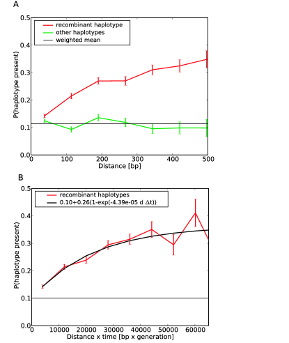
Figure 2: Estimating recombination rates from time resolved data. Panel A shows the probability of finding a haplotype that is not detected at time $t_{i}$ in the next time slice $t_{i+1}$ as a function of the separation $d$ of the sites. The data labeled ‘recombinant haplotypes’ refers to those combinations, that can be generated by recombination from the alleles detected at time $t_{i}$, and displays a pronounced distance dependence. The data labeled ‘other haplotypes’ refers to pairs containing at least one allele not detected at time $t_{i}$, implying an additional mutation or undersampling. The data is averaged over all time points, patients and those pairs of polymorphic sites, where both alleles at both sites are seen at least 3 times. Panel B shows the probability of finding the missing haplotype as a function of the product of distance $d$ and time interval $\Delta t=t_{i+1}-t_{i}$. The fit to the data is shown in black with fit parameters indicated in the legend.

The probability of recombination between two sites increases with the product of the time elapsed and the distance between the sites, rather than with distance alone as plotted in figure 2A. Panel B of figure 2 shows the probability of appearance of a putative recombinant haplotype as a function of the product of distance and number of generations (generation time 2 days). To estimate the recombination rate, we have to know how the observed saturation behavior is related to recombination. Let $a/A$ and $b/B$ be the alleles at site 1 and 2 and $p_{AB}$ the frequency of the missing haplotype $AB$. The probability not to detect haplotype $AB$ in a sample of size $M$ is

$$P(\mathrm{no\;AB})=(1-p_{AB})^{M}\approx e^{-Mp_{AB}}$$ (1)

Assuming the allele frequencies remain constant, $p_{AB}$ will relax from its initial value $p_{AB}^{0}$ to the product of the allele frequencies $p_{A}p_{B}$ as $p_{AB}(\Delta t)=p_{A}p_{B}+(p_{AB}^{0}-p_{A}p_{B})e^{-\rho d\Delta t}$ through recombination[26]. The frequency of detecting a haplotype at time $t_{i+1}$, given it was not detected in the previous sample at time $t=t_{i}$, is therefore ${\cal P}(d(t_{i+1}-t_{i}))=1-\langle e^{-Mp_{AB}(t_{i+1})}\rangle$. This quantity, averaged over all pairs of polymorphic sites at distance $d$ such that $d(t_{i+1}-t_{i})$ falls into a specified bin, is shown in figure 2B (the average extends over all patients and time points). To understand how ${\cal P}(d(t_{i+1}-t_{i}))$ depends on the recombination rate, it is useful to consider the two limiting cases of small and large $d\Delta t$

$${\cal P}(d\Delta t)=\begin{cases}\langle Mp_{AB}^{0}\rangle+\langle M(p_{A}p_{B}-p_{AB}^{0})\rangle\rho d\Delta t&\rho d\Delta t\ll 1\\ 1-\langle e^{-Mp_{A}p_{B}}\rangle&\rho d\Delta t\gg 1\end{cases}$$ (2)

where we assumed that $\langle Mp_{AB}^{0}\rangle$ is small compared to one (inspection of figure 2B shows this is true, we discuss this in more detail in Methods). Hence, the recombination rate is proportional to the slope $\alpha$ of ${\cal P}(d\Delta t)$ at $d\Delta t=0$. The intercept ${\cal P}(0)=\langle Mp_{AB}^{0}\rangle$ is simply the probability that we detect $AB$ at time $t_{i+1}$ in absence of recombination, given we missed it at time $t_{i}$. We determine the slope and the intercept by fitting the function $f(d\Delta t)=c_{0}+c_{1}(1-e^{-c_{2}d\Delta t})$ to the data. The recombination rate is then given by

$$\hat{\rho}=\frac{c_{1}c_{2}}{\langle Mp_{A}p_{B}\rangle-c_{0}},$$ (3)

where $\langle Mp_{A}p_{B}\rangle\approx 0.93$ is measured directly. The best fit yields $\hat{\rho}\approx 1.4\pm 0.6\times 10^{-5}$ recombinations per site and generation ($\pm$ one standard deviation). The uncertainty of $\hat{\rho}$ was estimated by resampling the patients with replacement 500 times. This bootstrap distribution of the recombination rate estimate is shown in figure 3. We have assumed that the allele frequencies $p_{A}$ and $p_{B}$ remain constant in the interval $[t_{i+1},t_{i}]$. We will see below, however, that some allele frequencies change rapidly. We expect that repeated sweeps will cause our method to overestimate the recombination rate: When the frequencies of the minor alleles increase, the missing haplotype is produced more rapidly then expected.

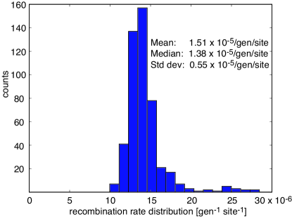
Figure 3: Bootstrap distribution of the recombination rate estimate. The variability of the recombination rate estimator was assessed by repeating the fit 500 times to data of eleven patients sampled with replacement from the original eleven patients. The mean, median and standard deviation of the distribution are given in the figure.

Selection

Positive selection on the variable regions in env and purifying selection on the conserved regions have been repeatedly reported in the literature [27, 5, 28, 29, 23]. Most of the these studies compared the rates of synonymous and non-synonymous substitutions ($dn/ds$ ratio). An observation of $dn/ds>1$ indicates selection for novel variants, while $dn/ds<1$ indicates that the amino acid sequence changes more slowly than the nucleotide sequence, indicating functional constraint at the protein level. The overall rate of substitutions, however, yields only very limited information about the strength of selection.

Selection for a specific variant implies that this variant confers an elevated rate of reproduction compared to the population mean. Ignoring random drift, the strength of selection $s$ is related to the rate at which the frequency $p$ of the variant changes [26]:

$$\frac{dp}{dt}=p(1-p)s$$ (4)

This equation has a straightforward solution $p(t)=e^{st}/(1+e^{st})$ and from two measurements of $p(t)$ at time $t_{i}$ and $t_{i+1}$, $s$ can be determined to be $s=\frac{1}{t_{i+1}-t_{i}}\ln\frac{p(t_{i})q(t_{i+1})}{q(t_{i})p(t_{i+1})}$ ($q=1-p$)[11] (for a review on selection and drift, see [30]). However, when using this formula, emphasis is put on rare alleles, whose frequencies can’t be measured accurately in small samples. It proves more robust to estimate the rate of allele frequency change directly as $\frac{\Delta p}{\Delta t}$, where $\Delta p$ is the difference in allele frequency between consecutive samples and $\Delta t$ is the time interval. The discrete derivative $\frac{\Delta p}{\Delta t}$ can serve as a proxy for selection which is less sensitive to rare alleles. The observed $\Delta p$ will be a sum of contributions from selection, noise from random sampling, and genetic drift. The latter can be estimated by measuring $\Delta p$ for synonymous polymorphisms which are putatively neutral and their observed frequency changes are assumed to be dominated by sampling noise. However, they can be affected by selection on nearby non-synonymous polymorphisms (hitch-hiking) or be themself under selection, e.g. for translation efficiency or RNA secondary structure.

Despite the limited resolution of $\Delta p$ and $\Delta t$ due to small sample sizes and large time intervals between samples (6-10 month), we can make a meaningful statement about the strength of selection when averaging over all sites, patients and time points. Figure 4 shows the cumulative distributions of the rates of change of allele frequencies observed during the interval between two consecutive time points for non-synonymous and synonymous polymorphisms. The histograms are shown as insets in the figure. There are consistently more fast changing non-synonymous polymorphisms than there are synonymous ones, suggesting that a fraction of the non-synonymous polymorphisms is indeed responding to selection. To check whether the fast changing synonymous polymorphisms can be attributed to hitchhiking, we excluded synonymous polymorphisms that are closer than 100bp to a non-synonymous polymorphism that changes faster than $0.002$ per generation. The resulting distribution is much narrower with no allele frequency changes beyond $0.003$ per generation, indicating that the fast changing synonymous polymorphisms are indeed “hitch-hiking”. The cumulative histograms can be compared by the Kolmogorov-Smirnov test, which uses the maximal vertical distance between curves as a test statistics. The test reveals that the non-synonymous distribution is significantly different from both the unconditional synonymous distribution (p-value $<10^{-13}$) and the synonymous distribution without hitch-hiking (p-value $<10^{-25}$). Note that not all observations are independent since nearby sites are linked and move coherently. Hence, realistic p-values will be larger.

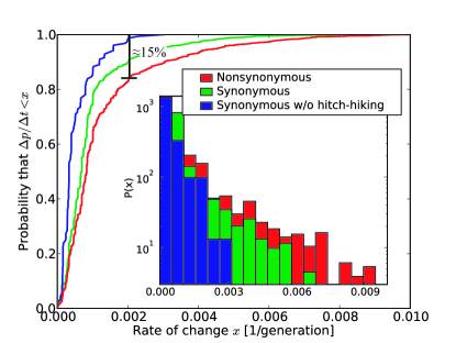
Figure 4: Selection on non-synonymous mutations. The figure shows cumulative distributions of the observed rate of change $\Delta p/\Delta t$ of the allele frequencies $p$ between two consecutive time points $t_{i}$ and $t_{i+1}$ for non-synonymous polymorphisms, synonymous polymorphisms and synonymous polymorphisms at least 100bp away from the nearest fast changing non-synonymous polymorphism ($>0.002$/generation), see methods. The insets show the corresponding histograms on a logarithmic scale. Only pairs of time points with sample sizes greater than 10 sequences are included.

The fastest allele frequency changes detected are about $0.01$ per generation, which is our resolution limit (6 month $\sim$ 100 generations). This low time resolution results in a tendency to underestimate the rates of change, while the finite sample size will generate spurious frequency changes due to sampling noise. However, the narrow distribution of allele frequency changes of synonymous polymorphisms excluding hitchkiking suggests that the contribution from sampling noise is small (on the order of $0.001$ per generation). Hence, the tail of the histogram of the frequency changes of nonsynonymous polymorphisms contains a rough measure of the distribution of selection coefficients[31]: about 15% of the observed non-synonymous polymorphisms change faster than $0.002$ per generation, compared to almost none of the synonymous polymorphisms. Assuming that this difference is due to selection, we conclude that about 15% of the observed non-synonymous polymorphisms are positively selected with $s>8\times 10^{-3}$ per generation. In the last step, we rearranged Eq. (4) to obtain $s\approx\frac{1}{p(1-p)}\frac{\Delta p}{\Delta t}\geq 4\times\frac{\Delta p}{\Delta t}$ with $p(1-p)\leq 0.25$. Most of the strongly deleterious polymorphism are of course never observed in the samples.

Discussion

The dynamics of HIV within a single patient is characterized by large diversity due to high mutation rates, intense selection, frequent recombination and stochasticity resulting from bursts of viruses originating from a single cell. The simultaneous importance of these four evolutionary forces makes HIV evolution difficult to analyze with traditional population genetic methods, which typically assume that one of the evolutionary forces is predominant. Coalescent based methods, for example, assume that evolution is neutral, i.e. stochasticity dominates over selection. While it is possible to include recombination or selection into a coalescent description [32, 33], the analysis becomes difficult and computationally demanding. Estimators based on site frequency spectra, like Tajima’s $D$, work best when recombination is strong compared to selection. Phylogenetic analysis, on the other hand, assumes absence of recombination. These methods have been designed to infer parameters of the population dynamics from snapshots of the population, which is a formidable challenge. The lack of time resolved data requires the assumption of a model of the population dynamics, which can be extrapolated back in time to the most recent common ancestor. In neutral models, the time to the most recent common ancestor is on the order of $N$ generations, $N$ being the population size. During this long time interval, there is ample opportunity for selection or demography to invalidate the assumption of the model.

If time resolved data is available, the task of estimating parameters is greatly simplified since one can trace the dynamics of alleles and genotypes directly. Such longitudinally sampled data has for example been used to gauge the molecular clock of bacterial evolution [34]. We have used time resolved data from 11 patients to estimate parameters of the population dynamics directly. In accordance with existing studies, we find that recombination in HIV is frequent and contributes significantly to sequence diversity [13, 11, 21, 12]. The template switching rate of HIV is known to be about $3\times 10^{-4}$ per site[18, 19]. For template switching to result in a novel genetic variant, the two RNA strands in the infecting virus have to be different, which implies co-infection of the cell the virus originated from. Any estimate of recombination rates from sequence diversity will therefore measure an effective recombination rate $\rho$ being approximately the product of the coinfection probability, the probability of forming a heterozygote and the template switching rate. Our estimate of this effective recombination rate is $\rho\approx 1.4\times 10^{-5}$ recombination per site and generation, which is about a factor of 20 lower than the template switching rate but still implies a probability of coinfection of about 10%. Our estimate is lower than the estimate by Shriner et al. [13], who estimated $\rho\approx 1.38\times 10^{-4}$ per site and generation. However, two other estimators also reported in that paper yielded lower recombination rates comparable to our estimate.

In our analysis we have assumed that the rate of recombination is constant across the env gene. However, the breakpoint distribution in circulating recombinant forms show strong variation along the genome, with particulary little recombination in env[35]. The variation of the breakpoint distribution can largely be explained by low sequence homology between different subtypes and dysfunctional recombinants [36]. In the present study, however, all patients were infected with a single subtype and gradually built up diversity which remained much lower than the distance between subtypes. The effects causing recombination rate variation should therefore be of minor importance.

By comparing the distribution of the rate of allele frequency changes of synonymous (putatively neutral) and nonsynonymous (possibly selected) polymorphisms, we estimated the distribution of selection coefficients on single sites. We find that 15% of the nonsynonymous polymorphism are selected with coefficients greater than $0.8$% per generation. In using the distribution of allele frequency changes to infer selection coefficients, we have assumed that each locus is selected for its own effect on fitness, rather than changing its frequency due to selection on a linked neighboring locus [37] or some epistatic combination of loci [38, 39]. A sweeping polymorphism “drags” along neutral variation in a region $s/\rho\log Ns$ [40], which using our estimates of $\rho$, $s\approx 0.01$ and an effective population size of $10^{4}$ evaluates to $200$bp. This is consistent with our finding that most of the rapid allele frequency changes of synonymous polymorphisms occur in the vicinity ($<100bp$) of rapidly changing non-synonymous polymorphisms (figure 4).

The sequence diversity in our samples is on the order of 3% [3], such that two polymorphisms are expected to be on average 30bp apart. Roughly half of the observed polymorphisms are non-synonymous, of which 15% are under strong positive selection. Hence the distance between simultaneously sweeping loci is on the order of 400bp, which is of the same order as $s/\rho$. If the rate of sweeps was much higher, sweeps would cease to be independent and interfere. While these estimates have large uncertainty, it is conceivable that the rate of sweeps is limited by recombination.

Selection coefficients in HIV have been estimated before by Liu et al. [11] in a patient infected with two HIV-1 subtype B viruses. In this patient, a small number of recombinant forms competed against the ancestral strains and selection differentials were estimated to lie between $0.3$% and $9$%. These selection coefficients are higher than our estimates, which is plausible since they are associated with entire recombinant genomes that differ at many sites rather than the single site estimate presented here. The strength of selection for novel epitopes in several HIV genes (rate of escape from cytotoxic T-lymphocyte mediated killing) during the asymptomatic phase of HIV infection has been shown to be of similar magnitude as our estimates [41].

The present study is limited by low time resolution and small sequence samples and more accurate and detailed answers could be obtained from larger samples. Larger sample sizes will require generalizations of the method used to estimate recombination rates which depends on pairs of sites where one of the four possible haplotypes is absent. In large samples, high frequency variants will most likely be present in all four possible haplotypes. In this case, one can measure linkage disequilibrium $D$ directly and observe how it decays from one timepoint to the next, e.g. by measuring its autocorrelation function $\langle D(t_{i})D(t_{i+1})\rangle=\langle D^{2}\rangle e^{-\rho d\Delta t}$. The method presented here is an approximation of this more general method suiteable for noisy data.

Methods

Longitudinal sequence data and alignment

Sequences of the C2-V5 region of env from 11 patients, which were part of the MACS study [22, 3], were obtained from the Los Alamos National Lab HIV data base (Special interest alignments, accession numbers: AF137629-AF138703, AF204402-AF204670, AY449806 - AY450055 & AY450056 - AY450257). The sequences were translated into amino acid sequences and aligned for each patient separately using MUSCLE v3.6 with default settings [42]. Aligned nucleotide sequences were then constructed by inserting a 3bp gap for each gap in the amino acid alignment. Scripting and plotting was done in Python using the NumPy and Matplotlib environment [43, 44].

Estimating the recombination rate

To estimate recombination rates, we calculated the frequency of generating the missing haplotype as a function of the distance between polymorphic sites. Specifically, the algorithm proceeds as follows: For each pair of biallelic and gapless sites, we constructed a list of haplotypes, i.e. a list of alleles that co-occur in the same sequence. The list typically contains 3 or 4 haplotypes, but can also contain only 2 of the 4 possible pairs due to undersampling or selection against some of the allele combinations. Only those pairs with 3 haplotypes were included in the estimation. Furthermore, we used only those sites where both alleles were observed at least three times, since rare alleles are very sensitive to sampling noise. The analysis was repeated with this cutoff at two or four alleles, yielding similar results.

For each pair of biallelic sites for which 3 haplotypes were detected in the sample in timeslice $t_{i}$, we determined the 4th haplotype that can be formed from the alleles observed at time $t_{i}$, i.e. C…G in the example given in Figure 1. We then checked whether this missing haplotype is detected in timeslice $t_{i+1}$. By averaging over all time points (but the last one), patients and pairs within a given distance interval, we determined the frequency of finding the missing haplotype as a function of the distance between the sites and as a function of the product of distance and time difference. The error bars indicated in figure 2 are calculated as the product of the estimated value and $1\pm\#\mathrm{counts}^{-0.5}$. This would be $\pm$ one standard deviation if all counts were independent, which they are not since the observations are pairs of sites and each site contributes to multiple pairs. However, these error bars indicate the relative uncertainties of the different points, which is all that is needed for an unbiased fit. According to eq. 2, we can estimate the recombination rate from the axis intercept and the slope at $d\Delta t=0$, which are extracted from the data by fitting

$$f(d\Delta t)=c_{0}+c_{1}(1-e^{-c_{2}d\Delta t})$$ (5)

to the data. The fit is done by minimizing the squared deviation, weighted by the relative uncertainty of the data points indicated by the error bars in figure 2. $\langle Mp_{A}p_{B}\rangle$ was averaged over all pairs of sites contributing. To estimate a confidence interval for the estimate of $\hat{\rho}$, the estimation was repeated 500 times with a set of 11 patients sampled with replacement from the original 11 patients.

The method relies on pairs of biallelic sites in a sample of size $M$, where 3 out of the 4 possible haplotypes are observed. In large samples from a recombining population, one would naively expect to observe all possible haplotypes. However, due to the very skewed allele frequency distributions $\sim\frac{1}{p(1-p)}$, the haplotype formed by the rare alleles is often sufficiently rare that it is missed even in large samples. We denote the alleles at site 1 by $a/A$ and at site 2 by $b/B$, with the $A$ and $B$ being the minor alleles. First, observe that the mean frequency of haplotype $AB$, $\langle p_{AB}\rangle$, at linkage equilibrium is $\langle p_{A}\rangle\langle p_{B}\rangle\approx\frac{\log^{2}2}{\log^{2}M}$. Hence $M\langle p_{AB}\rangle\approx 1$ for $M\leq 20$, in accord with $M\langle p_{A}\rangle\langle p_{B}\rangle\approx 0.93$ observed in the data. We further assumed that the frequency of the unobserved haplotype, $p_{AB}^{0}$, is significantly smaller than $M^{-1}$. There are several reasons why $p_{AB}^{0}$ is typically significantly smaller than $\langle p_{A}\rangle\langle p_{B}\rangle$ and hence smaller than $M^{-1}$: (i) the condition that haplotype $AB$ is not observed pushes $p_{AB}^{0}$ down, (ii) minor alleles tend to be in negative linkage equilibrium if they are involved in selective sweeps, (iii) allele frequency spectra are even more skewed than $\sim\frac{1}{p(1-p)}$ due to purifying selection. The degree to which these 3 reasons reduce $p_{AB}^{0}$ can be best observed in figure 2B at small $d\Delta t$. The figure shows the probability to observe haplotype $AB$ at time $t_{i+1}$, given it was not observed at time $t_{i}$. At small $d\Delta t$, linkage disequilibrium is not yet broken down by recombination and the probability to observe haplotype $AB$ at time $t_{i+1}$ gives us a measure of $Mp_{AB}$ at time $t_{i}$, which is indeed much smaller than 1. Hence we can expand $\exp(-Mp_{AB})$ for small $d\Delta t$ in Eq. 2.

Estimating the distribution of selection coefficients

The distribution of the rate of change of allele frequencies was estimated from pairs of successive time slices with the following characteristics: (i) site biallelic without indels at time $t_{i}$ with no constraint on timeslice $t_{i+1}$, and (ii) monomorphic sites at time $t_{i}$ that are biallelic at time $t_{i+1}$ (without indels). In both cases there are two alleles $a$ and $A$ whose frequencies can be meaningfully compared. The difference in allele frequencies were calculated as $\Delta p_{a}=n_{a}(t_{i+1})/M(t_{i+1})-n_{a}(t_{i})/M(t_{i})$, where $n_{a}(t_{i})$ is the count of allele $a$ at time $t_{i}$ and $M(t_{i})$ is the sample size. Unless a third allele arose between $t_{i}$ and $t_{i+1}$ (case (i)), $\Delta p_{a}=-\Delta p_{A}$ and the common estimate of the rate of change, $|\Delta p_{a}|/\Delta t$, was added to the cumulative distribution. In rare cases where a third allele did arise, both $|\Delta p_{a}|/\Delta t$ and $|\Delta p_{A}|/\Delta t$ have been added. Sometimes, a nucleotide changed from one state to another between time $t_{i}$ or $t_{i+1}$ with no polymorphisms detected. In such a case, $\Delta p=1$ was added.

To detect the action of selection, we produced cumulative histograms of the rate of change in allele frequency for nonsynonymous and synonymous (putatively neutral) polymorphisms by averaging over all patients and pairs of consecutive time points and $t_{i}$ and $t_{i+1}$ with both $M(t_{i})$ and $M(t_{i+1})$ greater than $10$. We then tested for excess of fast changes among the nonsynonymous polymorphisms using the Kolmogorov-Smirnov test. The test statistic is the maximal vertical difference between the cumulative distributions $D$ divided by $\sqrt{1/m_{s}+1/m_{n}}$, where $m_{s}$ and $m_{n}$ are the number of observations of synonymous and non-synonymous polymorphims. The Kolmogorov-Smirnov test was performed using the statistics module of SciPy [45].

To assess the role of hitch-hiking of synonymous polymorphisms with nearby selected non-synonymous polymorphisms, we produced a list of positions of non-synonymous polymorphisms whose allele freqency changes faster than $0.002$ per generation between time $t_{i}$ and $t_{i+1}$. Synonymous polymorphism closer than 100bp to any of these position where excluded from the conditioned histogram.

References

- 1. Duffy S, Shackelton LA, Holmes EC (2008) Rates of evolutionary change in viruses: patterns and determinants. Nat Rev Genet 9: 267–276.
- 2. Perelson AS, Neumann AU, Markowitz M, Leonard JM, Ho DD (1996) HIV-1 dynamics in vivo: virion clearance rate, infected cell life-span, and viral generation time. Science 271: 1582–6.
- 3. Shankarappa R, Margolick JB, Gange SJ, Rodrigo AG, Upchurch D, et al. (1999) Consistent viral evolutionary changes associated with the progression of human immunodeficiency virus type 1 infection. J Virol 73: 10489–502.
- 4. Lee HY, Perelson AS, Park SC, Leitner T (2008) Dynamic correlation between intrahost HIV-1 quasispecies evolution and disease progression. PLoS Comput Biol 4: e1000240.
- 5. Nielsen R, Yang Z (1998) Likelihood models for detecting positively selected amino acid sites and applications to the HIV-1 envelope gene. Genetics 148: 929–36.
- 6. Chen L, Perlina A, Lee CJ (2004) Positive selection detection in 40,000 human immunodeficiency virus (HIV) type 1 sequences automatically identifies drug resistance and positive fitness mutations in HIV protease and reverse transcriptase. J Virol 78: 3722–32.
- 7. Bazykin GA, Dushoff J, Levin SA, Kondrashov AS (2006) Bursts of nonsynonymous substitutions in HIV-1 evolution reveal instances of positive selection at conservative protein sites. Proc Natl Acad Sci USA 103: 19396–401.
- 8. Edwards CTT, Holmes EC, Pybus OG, Wilson DJ, Viscidi RP, et al. (2006) Evolution of the human immunodeficiency virus envelope gene is dominated by purifying selection. Genetics 174: 1441–53.
- 9. Jung A, Maier R, Vartanian JP, Bocharov G, Jung V, et al. (2002) Multiply infected spleen cells in HIV patients. Nature 418: 144.
- 10. Chen J, Nikolaitchik O, Singh J, Wright A, Bencsics CE, et al. (2009) High efficiency of HIV-1 genomic RNA packaging and heterozygote formation revealed by single virion analysis. Proc Natl Acad Sci USA 106: 13535–40.
- 11. Liu SL, Mittler JE, Nickle DC, Mulvania TM, Shriner D, et al. (2002) Selection for human immunodeficiency virus type 1 recombinants in a patient with rapid progression to AIDS. J Virol 76: 10674–84.
- 12. Charpentier C, Nora T, Tenaillon O, Clavel F, Hance AJ (2006) Extensive recombination among human immunodeficiency virus type 1 quasispecies makes an important contribution to viral diversity in individual patients. J Virol 80: 2472–82.
- 13. Shriner D, Rodrigo AG, Nickle DC, Mullins JI (2004) Pervasive genomic recombination of HIV-1 in vivo. Genetics 167: 1573–83.
- 14. Kuiken C, Leitner T, Foley B, Hahn B, Marx P, et al., editors (2009) HIV Sequence Compendium 2009. Los Alamos National Laboratory, Theoretical Biology and Biophysics, Los Alamos, New Mexico.
- 15. Nora T, Charpentier C, Tenaillon O, Hoede C, Clavel F, et al. (2007) Contribution of recombination to the evolution of human immunodeficiency viruses expressing resistance to antiretroviral treatment. J Virol 81: 7620–8.
- 16. Rouzine IM, Coffin JM (2005) Evolution of human immunodeficiency virus under selection and weak recombination. Genetics 170: 7–18.
- 17. Althaus CL, Bonhoeffer S (2005) Stochastic interplay between mutation and recombination during the acquisition of drug resistance mutations in human immunodeficiency virus type 1. J Virol 79: 13572–8.
- 18. Jetzt AE, Yu H, Klarmann GJ, Ron Y, Preston BD, et al. (2000) High rate of recombination throughout the human immunodeficiency virus type 1 genome. J Virol 74: 1234–40.
- 19. Zhuang J, Jetzt AE, Sun G, Yu H, Klarmann G, et al. (2002) Human immunodeficiency virus type 1 recombination: rate, fidelity, and putative hot spots. J Virol 76: 11273–82.
- 20. Levy DN, Aldrovandi GM, Kutsch O, Shaw GM (2004) Dynamics of HIV-1 recombination in its natural target cells. Proc Natl Acad Sci USA 101: 4204–9.
- 21. McVean G, Awadalla P, Fearnhead P (2002) A coalescent-based method for detecting and estimating recombination from gene sequences. Genetics 160: 1231–41.
- 22. Kaslow RA, Ostrow DG, Detels R, Phair JP, Polk BF, et al. (1987) The multicenter AIDS cohort study: rationale, organization, and selected characteristics of the participants. Am J Epidemiol 126: 310–8.
- 23. Shriner D, Shankarappa R, Jensen MA, Nickle DC, Mittler JE, et al. (2004) Influence of random genetic drift on human immunodeficiency virus type 1 env evolution during chronic infection. Genetics 166: 1155–64.
- 24. Hudson RR, Kaplan NL (1985) Statistical properties of the number of recombination events in the history of a sample of DNA sequences. Genetics 111: 147–64.
- 25. Leitner T, Kumar S, Albert J (1997) Tempo and mode of nucleotide substitutions in gag and env gene fragments in human immunodeficiency virus type 1 populations with a known transmission history. J Virol 71: 4761–70.
- 26. Ewens WJ (2004) Mathematical Population Genetics: Theoretical introduction. Springer, Berlin.
- 27. Seibert SA, Howell CY, Hughes MK, Hughes AL (1995) Natural selection on the gag, pol, and env genes of human immunodeficiency virus 1 (HIV-1). Mol Biol Evol 12: 803–13.
- 28. Templeton AR, Reichert RA, Weisstein AE, Yu XF, Markham RB (2004) Selection in context: patterns of natural selection in the glycoprotein 120 region of human immunodeficiency virus 1 within infected individuals. Genetics 167: 1547–61.
- 29. Yamaguchi Y, Gojobori T (1997) Evolutionary mechanisms and population dynamics of the third variable envelope region of HIV within single hosts. Proc Natl Acad Sci USA 94: 1264–9.
- 30. Rouzine IM, Rodrigo A, Coffin J (2001) Transition between stochastic evolution and deterministic evolution in the presence of selection: General theory and application to virology. Microbiology amd Molecular Biology Reviews 65: 151–185.
- 31. Eyre-Walker A, Keightley PD (2007) The distribution of fitness effects of new mutations. Nat Rev Genet 8: 610.
- 32. Griffiths RC, Marjoram P (1996) Ancestral inference from samples of DNA sequences with recombination. J Comput Biol 3: 479–502.
- 33. Neuhauser C, Krone SM (1997) The genealogy of samples in models with selection. Genetics 145: 519–34.
- 34. Wilson DJ, Gabriel E, Leatherbarrow AJH, Cheesbrough J, Gee S, et al. (2009) Rapid evolution and the importance of recombination to the gastroenteric pathogen campylobacter jejuni. Mol Biol Evol 26: 385–97.
- 35. Archer J, Pinney JW, Fan J, Simon-Loriere E, Arts EJ, et al. (2008) Identifying the important HIV-1 recombination breakpoints. PLoS Comput Biol 4: e1000178.
- 36. Simon-Loriere E, Galetto R, Hamoudi M, Archer J, Lefeuvre P, et al. (2009) Molecular mechanisms of recombination restriction in the envelope gene of the human immunodeficiency virus. PLoS Pathog 5: e1000418.
- 37. Gillespie JH (2001) Is the population size of a species relevant to its evolution? Evolution 55: 2161–9.
- 38. Kimura M (1965) Attainment of quasi linkage equilibrium when gene frequencies are changing by natural selection. Genetics 52: 875–90.
- 39. Neher RA, Shraiman BI (2009) Competition between recombination and epistasis can cause a transition from allele to genotype selection. Proc Natl Acad Sci USA 106: 6866–6871.
- 40. Barton N (1998) The effect of hitch-hiking on neutral genealogies. Genet Res 72: 123–133.
- 41. Asquith B, Edwards CTT, Lipsitch M, McLean AR (2006) Inefficient cytotoxic t lymphocyte-mediated killing of HIV-1-infected cells in vivo. PLoS Biol 4: e90.
- 42. Edgar RC (2004) Muscle: multiple sequence alignment with high accuracy and high throughput. Nucleic Acids Res 32: 1792–7.
- 43. Oliphant T (2007) Python for scientific computing. Computing in Science & Engineering 9: 10–20.
- 44. Hunter J (2007) Matplotlib: a 2d graphics environment. Computing in Science & Engineering 9: 90–95.
- 45. Jones E, Oliphant T, Peterson P, et al. (2001–2009). SciPy: Open source scientific tools for Python. URL http://www.scipy.org/.