Competition between recombination and epistasis can cause a transition from allele to genotype selection

Abstract

Biochemical and regulatory interactions central to biological networks are expected to cause extensive genetic interactions or epistasis affecting the heritability of complex traits and the distribution of genotypes in populations. However, the inference of epistasis from the observed phenotype-genotype correlation is impeded by statistical difficulties, while the theoretical understanding of the effects of epistasis remains limited, in turn limiting our ability to interpret data. Of particular interest is the biologically relevant situation of numerous interacting genetic loci with small individual contributions to fitness. Here, we present a computational model of selection dynamics involving many epistatic loci in a recombining population. We demonstrate that a large number of polymorphic interacting loci can, despite frequent recombination, exhibit cooperative behavior that locks alleles into favorable genotypes leading to a population consisting of a set of competing clones. When the recombination rate exceeds a certain critical value that depends on the strength of epistasis, this ”genotype selection” regime disappears in an abrupt transition, giving way to ”allele selection”-the regime where different loci are only weakly correlated as expected in sexually reproducing populations. We show that large populations attain highest fitness at a recombination rate just below critical. Clustering of interacting sets of genes on a chromosome leads to the emergence of an intermediate regime, where blocks of cooperating alleles lock into genetic modules. These haplotype blocks disappear in a second transition to pure allele selection. Our results demonstrate that the collective effect of many weak epistatic interactions can have dramatic effects on the population structure.

Selection acting on genetic polymorphisms in populations is a major force of evolution McDonald_Nature_1991 ; Begun_PlosBiology_2007 ; Gerrish_Genetica_1998 ; Desai_Genetics_2007 and it is possible to identify specific loci under positive selection (e.g. the Adh locus in Drosophila McDonald_Nature_1991 ). Yet, the attribution of fitness differentials to specific allelic variants and combinations remains a great challenge Mackay_NatRevGen_2001 . Efforts to correlate quantitative phenotypes with genetic polymorphisms typically identify a small number of loci with a significant contribution to the observed phenotypic variance, but leave much of the variance unaccounted for Barton_NatRevGen_2002 . This unaccounted variance is believed to arise from a large number of loci with small individual contributions, or be due to epistasis and quite likely involves both effects. New studies accumulate evidence that epistasis is widespread and accounts for a significant fraction of phenotypic variation (e.g. in yeast Brem_Nature_2005 ; Segre_NatureGenetics_2005 ; Schuldiner_Cell_2005 ). Additional evidence for epistasis comes from crosses of mildly diverged strains, where the recombinant progeny often has reduced average fitness, i.e.  display outbreeding depression. The reduction in fitness is attributed to the breakdown of favorable combination of alleles in the ancestral strains Dobzhansky_Genetics_1950 . Outbreeding depression is often observed in partly selfing organisms such as C. elegans Dolgin_Evolution_2007 or plants Parker_Evolution_1992 , species with strong geographic isolation such copepod Edmands_JHered_2008 or facultatively mating organisms such as yeast Kuehne_CurrentBiology_2007 . While most recombinant genotypes are less fit, novel genotypes that perform better than either parental strain can be generated as well Wright_Genetics_1931 . Such outcrossing events could play an important role in evolution.

Competition between epistatic selection and recombination, explicit in the outbreeding depression phenomenon, is the focus of the present study. In the presence of epistasis, selection, by increasing the frequency of favorable genotypes, establishes correlations between alleles at different loci. Recombination on the other hand reshuffles alleles and randomizes genotypes breaking up coadapted loci. Because recombination rate between any two loci is largely determined by their physical distance on the chromosome, the effect of genetic interactions depends on gene location. It is known that functionally related genes tend to cluster Roy_Nature_2002 ; Hurst_NatRevGen_2004 , suggesting selection on gene order. Furthermore, chromosomes have regions of infrequent recombination, interspersed with recombination hotspots HapMap . Does selection have a hand in defining low recombination regions? To understand how evolution shaped genomes as we observe them today, we have to tackle the problem of how selection acts on many interacting polymorphisms for a large range of recombination rates Slatkin_NatRevGen_2008 .

Standing variation harbored in natural population provides important raw material for selection to act upon, in particular after a sudden change in environments or hybridization events Teotonio_NatGen_2009 . In such a situation, selection will reduce genetic variation until a new mutation-selection equilibrium is reached. Here, we show that the selection dynamics on standing variation at a large number of loci can be strongly affected by epistasis, even if the individual contribution of each locus is small. The competition between selection on epistasis and recombination gives rise to two distinct regimes at high and low recombination rates separated by a sharp transition. The population dynamics in the two regimes is illustrated in Fig. 1a,b: i) the “clonal competition” (CC) regime which occurs for recombination rates $r<r_{c}$ and ii) the Quasi Linkage Equilibrium (QLE) regime for $r>r_{c}$. The different nature of the two regimes is best understood by considering the limiting cases of no and frequent recombination. In the case of purely asexual reproduction, selection operates on entire genotypes and results in clonal expansion of the fitter ones. The genetic variation present in the initial population is lost on a timescale inversely proportional to the average magnitude of fitness differentials between genotypes present in the population. Successful genotypes persist in time, which is apparent as continuous broad stripes of one color in Fig. 1a. The amplification of a small number of fit genotypes induces strong correlations or linkage disequilibrium among loci. In presence of epistasis, a little recombination does not change this picture qualitatively, as most recombinant genotypes are less fit than the prevailing clones and novel successful clones are rare. Nevertheless recombination is very important because it continuously introduces new genotypes leading to an increase in fitness attained by the population at long times. In the limit of high recombination genotypes are short-lived and essentially unique, resulting in a “pointillist” color pattern in Fig. 1b. Each allelic variant is therefore selected on the basis of its effect on fitness, averaged over many possible genetic backgrounds. The time scale on which allele frequencies change is given by the inverse of these marginal fitness effects. The term ”linkage equilibrium” in QLE refers to the negligible correlations between loci, which are constantly reshuffled by recombination.

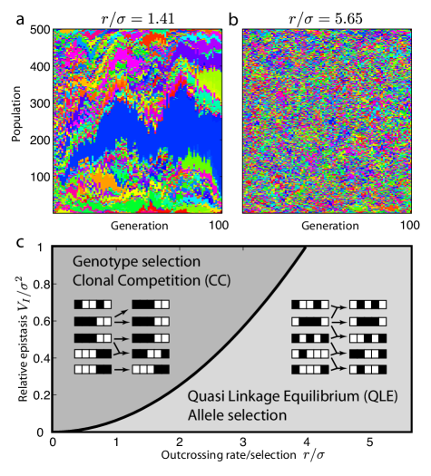
Figure 1: The two regimes of sexual reproduction. Panels a & b show the simulated time course of the genotype distribution in a population of 500 individuals with epistatic fitness variance $V_{I}=\sigma^{2}=0.005$ and the outcrossing rate $r=0.1$ (a) and $r=0.4$ (b). Like genotypes are assigned the same color and stacked on top of each other. Sketches illustrating the population dynamics in the two cases are shown as insets in panel c. At low outcrossing rates, fit genotypes can proliferate. The genotype distribution rapidly coarsens and clones form (horizontal stripes in panel a). With frequent outcrossing, genes are rapidly reshuffled and genotypes do not persist over many generations, resulting in the pointillist pattern in panel b. Fixation happens at later time and is not shown. Panel c: The two regimes are separated by a sharp boundary set by the strength of epistasis. For $r<r_{c}$, the population dynamics is described by clonal competition (CC); for $r>r_{c}$ by quasi linkage equilibrium (QLE).

As we show below, the transition between the two regimes sharpens as the number of segregating loci $L$ increases. The sharpening of the transition is related to the different scaling of the time scale of selection in the two regimes. For large $L$, the marginal fitness effects of individual loci become small compared to fitness differentials among individuals (assuming they are all of similar size, this ratio decreases as $\sim 1/\sqrt{L}$). Hence, the dynamics in the QLE regime slows down compared to the CC regime as $L$ increaes. The CC and QLE regimes correspond to different regions of the parameters space spanned by the relative strength of epistasis and the ratio of outcrossing or recombination rate to the strength of selection, as sketched in Fig. 1c. The QLE dynamics was first described by Kimura Kimura_Genetics_1965 in the limit of weak selection/fast recombination for a pair of bi-allelic loci and subsequently generalized to multi-loci systems Barton_Genetics_1991 ; Nagylaki_Genetics_1993 . The possibility of a collective behavior involving linkage disequilibrium on many loci and selection effectively acting on the whole chromosome as a unit has been pointed out before in the context of overdominance by Franklin and Lewontin Franklin_Genetics_1970 in the strong selection limit. However, these studies of the two different limits do not reveal the breakdown of QLE and the transition to CC as the generic behavior of multi-locus epistatic systems.

To underscore the general nature of the results, we shall consider two different models of epistasis. The first model will follow the common treatment of epistasis in quantitative traits which assumes that the epistatic contribution to fitness is disrupted when the parental genes are mixed in sexual reproduction Lynch_1998 ; Falconer_1996 . This assumption becomes exact when the epistatic component of fitness of a specific genotype is a random number (which depends on the genotype, but is fixed in time) and we shall call this model the random epistasis (RE) model. Within the RE model, any change in the genotype randomizes the epistatic component of fitness so that the latter is not heritable when non-identical parents mate. It is, however, faithfully passed on to the offspring in asexual reproduction. For the RE model, genomes are propagated asexually with probability $1-r$ and with probability $r$ are a product of mating where all genes are reassorted, as would be exactly correct if all genes were on different chromosomes. This model of facultative mating approximates reproductive strategies common in fungi (e.g. yeast) or nematodes and plants. As a more realistic alternative, we shall also study a model with only pairwise interactions between loci Hansen_TheoPopBiol_2001 . This pairwise epistasis (PE) model allows epistatic contribution to be partly heritable, as interacting pairs have a chance to be inherited together Bulmer_1980 . For the PE model, we assume that all genes are arranged on one chromosome with a uniform crossover rate $\rho$, which allows us to explore haplotype block formation and implications for recombination rate evolution.

The strength of selection is determined by the variance $\sigma^{2}$ of the distribution of fitness in the population. Within our models, the fitness $F(g)$ of a genotype $g$ is the sum of an additive component $A(g)$ representing independent contributions of alleles and an epistatic part $E(g)$. For the RE model, the latter is a random number drawn from Gaussian distribution, while for the PE model it is a sum of pairwise interactions with random coefficients $f_{ij}$. The variances $V_{A}$ and $V_{I}$ of the distributions of $A(g)$ and $E(g)$ add up to $\sigma^{2}$ and their relative magnitude determines the importance of additive effects compared to epistasis. The two different models and their parameters are given explicitly in the methods section. For the sake of simplicity, we assume haploid genomes. Random and pairwise epistasis represent two opposite extremes in the complexity of epistasis. While the pairwise model is more realistic, the generic behavior is most clearly demonstrated using the RE model with random gene reassortment and facultative mating.

1 Results

Two regimes of selection dynamics.

We performed extensive computer simulation of our two models for different relative strength of epistasis, $L=25-200$ loci and populations sizes between $N=500$ and $10^{6}$. We initialize simulations in a genetically diverse state as would result from multiple crossings of two diverged strains and examine the evolution under selection and recombination. The two regimes differ strongly in the amount of linkage disequilibrium (LD) (see Methods) build up by selection. Panel a of Fig. 2 shows the average LD per locus pair for the RE model as a function of the outcrossing rate $r$. For $r<r_{c}$, the LD per locus pair is of order one and independent of $L$ or $N$, indicating genome-wide LD. LD builds up despite a large number of different genotypes in the population interbreeding constantly. For $r>r_{c}$, the LD is much smaller, with the observed value determined by the sampling noise due to the finite population size (see inset of Fig 2a and supplementary Figure S1). Similar behavior occurs in the PE model, as shown in panel b. Above a critical recombination rate $\rho_{c}$, the observed linkage disequilibrium is time independent and well described by the QLE approximation Kimura_Genetics_1965 ; Barton_Genetics_1991 (straight line, see supplement). The QLE approximation (in the high $\rho/\sigma$ limit) predicts LD to be proportional to the strength of pairwise epistasis Below $\rho_{c}$, the observed LD is dramatically larger than the QLE expectation. Here, recombination is sufficiently infrequent such that genotypes with a synergistic alleles are amplified faster than they are taken apart by recombination, see below. As a result, the few fittest genotypes grow exponentially in number, leading to the strong correlation in the occurrence of cooperating alleles, independent of physical linkage (i.e. proximity on the chromosome). This extensive LD leads to a complete failure when extrapolating results valid in the high recombination regime across the transition. The relevant quantity that determines whether fit genotypes can be maintained is the probability that no crossover occurs, which is given by $e^{-\rho L}$. Hence, $\rho_{c}$ is inversely proportional to $L$.

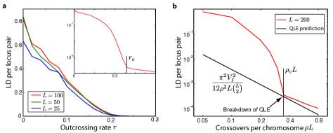
Figure 2: The clonal competition regime is characterized by extensive linkage disequilibrium. a Random epistasis model: For small $r$, the LD per locus pair is of order one and fairly independent of $L$. The inset shows the data for $L=100$ on a logarithmic scale and a mark at the value of $r_{c}$. The LD for $r>r_{c}$ is due to sampling noise, see Figure S1. b Pairwise epistasis model: For pairwise epistasis, the QLE approximation gives explicit predictions for LD, which describes the observed LD very accurately for $\rho>\rho_{c}$, black line. For $\rho<\rho_{c}$, LD is a much larger than the QLE prediction. For both panels, LD is measured when allelic entropy has decayed 30% from the initial value ($\sigma^{2}=0.005$, $V_{A}=0.1\sigma^{2}$ and $V_{I}=0.9\sigma^{2}$). In panel a, $N=10^{5}$ and the data shown is averaged over 100 realizations. To avoid boundary and finite size effects, we used $N=10^{6}$ and a circular chromosome for panel b and averaged over 10 realizations.

Self-consistency condition for QLE.

The fitness of a genotype can be decomposed as $F=A+E$, where $A$ is the heritable additive part and $E$ is the non-heritable epistatic part. As a coarse-grained descriptor of the population, we consider the joint distribution $P(A,E;t)$ of the fitness components. In the QLE state, $P(A,E;t)$ evolves approximately as

$$\partial_{t}P(A,E;t)=(F-\bar{F}-r)P(A,E;t)+r\rho(E)\vartheta(A;t)$$ (1)

The first term accounts for the exponential growth of genotypes with fitness advantage $F-\bar{F}$ and the loss due to recombination at rate $r$. The second term accounts for the production of genotypes through recombination. To a good approximation, the distribution of $A$ among recombinant offspring is identical to that among the parents $\vartheta(A)=\int dE\;P(A,E)$, which in turn is approximately Gaussian Turelli_Genetics_1994 . The distribution of $E$ among recombinant offspring is independent of the parents and a random sample from the distribution of epistatic fitness $\rho(E)$, which in our models is a zero-centered Gaussian. The latter is exactly true for the RE model and holds approximately for the PE model, where the correlation of $E$ between ancestor and offspring halves every generation Bulmer_1980 . Eq. (1) admits the factorized solution $P(A,E;t)=\vartheta(A;t)\omega(E)$ with $\partial_{t}\vartheta(A;t)=(A-\bar{A})\vartheta(A;t)$ and a time-independent distribution of $E$

$$\omega(E)=\frac{r\rho(E)}{r+\bar{E}-E},$$ (2)

where $\bar{E}$ is determined by the condition that $\omega(E)$ has to be normalized. This solution exists only if $E<r+\bar{E}$ for all genotypes; otherwise, fit genotypes escape recombination and grow as clones. These two scenarios are illustrated in Fig. 3.

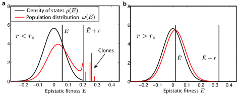
Figure 3: The break-down of QLE. Panel a: When the recombination rate decreases below $r_{c}$, some individuals have epistatic fitness $E$ larger than $\bar{E}+r$, and the QLE solution for the distribution of epistatic fitness in the population breaks down. Individuals to the right of $\bar{E}+r$ form clones that grow exponentially and the population condenses into a small number of genotypes. Panel b: For $r>r_{c}$, even the largest epistatic fitness contributions do not result in a growth advantage that exceeds the recombination rate.

The normalization condition can be fulfilled only if $r$ is larger than some $r_{c}$. The value of $r_{c}$ is proportional to the maximal $E$ and hence proportional to the strength of epistasis $\sqrt{V_{I}}$. However, it is not the absolute maximum of $E$ among all possible $2^{L}$ genotypes that determines $r_{c}$, but the maximal $E$ that is encountered by the population before fixation. Hence $r_{c}$ depends on the population size and the functional form of this dependence is determined by the upper tail of the distribution $\rho(E)$. For the Gaussian distribution used here, $r_{c}\sim\sqrt{\ln(rN\tau)}$, where $\tau$ is the time scale of QLE dynamics discussed below.. The product $rN\tau$ then is the number of genotypes generated through recombination before fixation. A more detailed discussion is given in the Supplementary information.

The breakdown of the QLE state has some similarity to the error-threshold transition of a quasi-species model Eigen_Naturwissenschaften_1971 in a rugged fitness landscape Franz_JPA_1997 : Recombination of epistatic loci acts as deleterious mutations and prevents the emergence of quasi-species or clones Boerlijst_PRSB_1996 ; Park_PRL_2007 for $r>r_{c}$.

Maintenance of genetic diversity.

The transition between the two regimes leaves its imprint in virtually every quantity of interest in population genetics. For instance, the characteristic time for the decay of genetic diversity, $\tau$, (which we quantify via allele entropy, see Methods) scales differently with $L$ in the two regimes, as shown in Fig. 4. At low outcrossing rates, $\tau$ depends only on the total variance in fitness and neither on the number of loci nor the relative strength of additive contributions. This is consistent with the notion that in the CC regime genotypes are the units on which selection acts. With more frequent outcrossing, $\tau$ tends to be larger for weak additive contributions and large $L$. Beyond a certain outcrossing rate $r_{c}$, $\tau$ becomes independent of $r$ attaining a value inversely proportional to the additive contribution of the individual loci independent of $V_{I}$ (black diamonds in Fig 3a). This observation confirms our assertion that for $r>r_{c}$, outcrossing decouples the loci and that the allele frequencies evolve independently under the action of the additive component of fitness. Given an additive variance $V_{A}$, the typical single locus fitness differential is $f\sim\sqrt{V_{A}/L}$ such that $\tau$ grows as $\sqrt{L}$ for $r>r_{c}$. To uncover the universal behavior in the vicinity of the transition in the limit of large genomes, we show that the data for different $V_{I}$, $V_{A}$ and $L$ collapses onto a single master curve after appropriate rescaling of the axis, see Fig. S2. This scaling collapse demonstrates the existence of a sharp transition in the limit $L\to\infty$, the scaling of $\tau$ with $\sqrt{L}$ and shows that $r_{c}$ is proportional to $\sqrt{V_{I}}$, as expected from the self-consistency argument outlined above and sketched in Fig. 1c. The suppression of allele dynamics by $1/\sqrt{L}$ in the QLE regime is at the basis of Fisher’s infinitesimal model put forward to explain sustained response to selection Barton_NatRevGen_2002 . In one generation, the allele frequencies change by approximately $f$, which can be sustained over $\sim f^{-1}$ generations. The mean fitness increases by $V_{A}$ per generation, consistent with Fisher’s theorem Lynch_1998 ; Nagylaki_Genetics_1993 . Our results show, that epistasis causes the breakdown of the infinitesimal model for $r<r_{c}$. The pairwise epistasis model is more complex than the random epistasis model, since the partition of the fitness variance in additive and epistatic contribution depends on the allele frequencies and epistasis is “converted” into additive fitness as the population approaches fixation Turelli_Evolution_2006 (a detailed account will be published elsewhere).

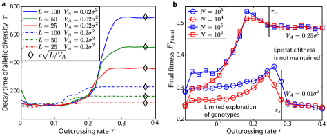
Figure 4: Panel a shows the time $\tau$ it takes to reduce the allelic entropy by 30% as a function of $r$ for different parameters. For small $r$, $\tau$ is independent of $L$ but increases with $r$. For $r>r_{c}$, $\tau$ settles at $c\sqrt{L/V_{A}}$ (black diamonds) in accord with the theoretical prediction for single locus dynamics (with c a fitting parameter). Additional data for $V_{A}=0$, $V_{A}=0.5\sigma^{2}$ and a collapse confirming the scaling of $\tau$ is shown in supplementary figure S2. Panel b: The fitness of the fixated genotype $F_{\rm{final}}$ as a function of $r$ for two different strength of epistasis. At $r=0$, the final fitness only depends on the population size $N$ and is independent of the strength of epistasis. $F_{\rm{final}}$ increases with $r$, followed by a pronounced drop right below $r_{c}$. Above $r_{c}$, $F_{\rm{final}}$ is almost constant and is independent of $N$. In both panels, $\sigma^{2}=0.005$. Data is averaged over 25 realizations in panel a and over 100 realizations in panel b. $L=100$ in panel b.

The properties of the genotype which will eventually fixate in the population depends on the regime in which it was obtained. We find, that the fitness of this fixated genotype depends non-monotonically on the outcrossing rate and peaks just below the transition, see Fig. 4. This can be understood as follows. Without recombination, the final state can be no fitter than the fittest genotype initially present. With some recombination, the population explores a greater number genotypes, potentially finding ones with higher fitness so that the fitness of final state increases with $r$ in the CC regime. A similar benefit of infrequent recombination due to exploration of genotype space has been studied in the context of virus evolution for additive fitness functions Rouzine_Genetics_2005 . As genotype selection gives way to allele selection, different loci decouple and the epistatic contribution to fitness is missed, leading to possible fixation of less fit genotypes and a sharp drop of the final fitness $r$ approaches $r_{c}$. The dependence of the final fitness on the population size $N$ highlight the distinct properties the dynamics in the two regimes: In the QLE regime, the final fitness is virtually identical for different $N$. This is a consequence of the fact that the relevant dynamical variables are allele frequencies, which are well sampled by $\mathcal{O}(N)$ individuals. Fluctuation of the allele frequencies are therefore negligible and the dynamics is essentially deterministic. This is different in the CC regime, where the dynamics is driven by the generation of rare, exceptionally fit genotypes. The rate, at which genotypes are generated is proportional to the $N$, resulting in a pronounced dependence on the population size. QLE ceases to be deterministic once the marginal fitness effects become comparable to inverse population size and random genetic drifts overwhelms selection, see Fig. S3 in the Supplementary information.

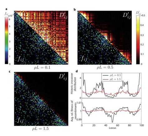
Figure 5: Clonal competition, modular selection and quasi linkage equilibrium. Above the diagonal, panels a, b and c show the LD measured as $D_{ij}^{\prime}$ between two loci $i$ and $j$ for a linear chromosome of length $L=100$ at three different crossover rates $\rho$. Below the diagonal, the interaction matrix $f_{ij}$ is shown (the same in all three panels). At low $\rho$, the sparse long range interactions suffice to produce genome wide LD. At intermediate $\rho$, distant part of the genome are decoupled, but the more strongly interacting clusters still show high LD, which vanishes at even higher recombination rates. Panel d, top: the distribution of historic crossovers. Bottom: The relative fitness of recombinants as a function of the crossover location. LD was measured when allelic entropy was at 90% of the initial value, $\sigma^{2}=V_{I}=0.005$ and $N=10^{6}$.

Selection on genetic modules.

So far, we assumed that each pair of loci is equally likely to interact epistatically, regardless of their physical distance on the chromosome. However, there is evidence that the order of genes along the chromosome is far from random and that related genes tend to cluster Roy_Nature_2002 ; Hurst_NatRevGen_2004 . To emulate such a situation we use the PE model and construct an interaction matrix $f_{ij}$ where arbitrary pairs interact with a small probability while clusters of neighboring genes interact with a high probability (see Methods). For such a hierarchical epistatic structure, we observe, as a function of increasing crossover rate $\rho$, a sequence of two transitions which define, sandwiched between CC and QLE, an intermediate Modular Selection (MS) regime, where the genome-wide LD characteristic of the CC regime has broken down to a set of modular blocks which are in quasi linkage equilibrium with each other. The resulting linkage disequilibrium patterns are shown in Fig. 5. The observed block structure of LD in the MS regime resembles haplotype blocks HapMap ; Slatkin_NatRevGen_2008 , which are normally associated with regions of little recombination flanked by recombination hotspots. Indeed, the cumulative recombination history of the chromosomes in the population show a very heterogenous recombination distribution, as shown in panel d of Fig. 5. Yet, here the origin of these blocks is not intrinsically low recombination (i.e. physical linkage) but the collective effect of epistatic selection: the surviving individuals have recombined more often in regions of low epistasis than in regions of high epistasis, even though the attempted crossovers are uniformly distributed along the chromosome. Clusters of epistatic interaction can therefore exert selective pressure to lower recombination within the cluster. This lack of recombinant survival has been observed in experiments with mice Petkov_PLOSgenetics_2005 , where inbreeding results in strong selective pressure on localized clusters of genes generating blocks with high LD and reduced effective recombination.

2 Conclusion

To summarize, we have shown that the competition of epistatic selection and recombination can give rise to distinct regimes of population dynamics, separated by a transition that becomes sharp for large number of interacting loci. The QLE and CC regimes are realizations of the opposing views on evolution of R.A. Fisher and S. Wright. For $r>r_{c}$ alleles are selected for the their additive contributions while selection acts on whole genotypes for $r<r_{c}$. The fundamental differences between these two regimes show up most clearly in the different scaling properties of the total LD and the decay time of genetic diversity. In the low recombination regime, LD is produced independent of physical linkage by the collective effect of many interactions. In the high recombination regime, LD can be attributed to specific interactions between pairs of loci and its value, determined by the ratio of the interaction strength and the rate of recombination between the loci, is small. Our results not only apply to the transition between genotype and allele selection, but also to localized clusters of interacting genes on the chromosome. Whenever the epistatic fitness difference between different allelic compositions of a cluster exceeds the recombination rate of the cluster, the fittest will amplify exponentially. Since such clusters are often small Petkov_PLOSgenetics_2005 ($\sim$ Mb) their recombination rates are low (cM or less) - hence fitness differentials below one percent can suffice to establish CC dynamics. Selective pressure to reduce recombination load, i.e. the fitness loss through recombination, will therefore favor the evolution of clusters of interacting genes and might be an important driving force for the evolution of recombination rate Nei_Genetics_1967 ; Barton_Genetics_2005 . The effects described above may provide an explanation for the functional clustering associated with low and high LD regions reported in HapMap HapMap .

Methods

Random epistasis model.

A genotype $g$ is described by $L$ binary variables $s_{i}=\pm 1$, $i=1,\ldots,L$. To each genotype we assign a fitness

$$F(g)=f\sum_{i}^{L}s_{i}+\xi(g).$$ (3)

The first term is the sum of the additive fitness contributions of the individual loci, each of which has equal magnitude $f=\sqrt{V_{A}/L}$. The second term is the non-heritable epistatic fitness, where $\xi(g)$ is drawn from a normal distribution with zero mean and variance $V_{I}$. For a uniform distribution of genotypes, the additive fitness variance is $V_{A}$, the epistatic variance is $V_{I}$, and the total variance is $\sigma^{2}=V_{A}+V_{I}$.

Pairwise epistasis model.

Here, we consider epistasis due to pairwise interactions between the different loci. Such pairwise interactions correspond to $s_{i}s_{j}$ terms in the fitness function. The fitness of a particular genotype $g$ is determined by the independent effects of the individual loci and the sum of the interactions between all pairs.

$$F(g)=f\sum_{i}^{L}s_{i}+\sum_{i<j}f_{ij}s_{i}s_{j}.$$ (4)

When assuming uniform epistasis between all possible pairs, we draw the interaction strength $f_{ij}$ from a Gaussian distribution with zero mean and variance $\frac{2V_{I}}{L(L-1)}$.

Clustered epistasis.

To mimic localized clusters of strongly interacting genes on a weakly interacting background, we constructed the matrix of $f_{ij}$’s as follows. The sparse background epistasis was modeled by assigning each $f_{ij}$ a Gaussian random number with probability $p=0.1$ and zero otherwise. Then we built three epistatic clusters with centers $c_{k}=10,50,90$ by adding a Gaussian random number to each $f_{ij}$ with probability $p=\exp\left(\frac{(i-c_{k})^{2}+(j-c_{k})^{2}}{2r^{2}}\right)$ with $r=10$ for $k=1,2,3$. All $f_{ij}$ were rescaled such that $\sum_{i<j}f_{ij}^{2}=V_{I}$.

Selection.

Our model assumes non-overlapping generations. In each generation a pool of gametes is produced, to which each individual contributes a number of copies of its genome which is drawn from a Poisson distribution with parameter $\exp(F(g)-\bar{F})$.

Gene re-assortment.

To model gene re-assortment in a facultatively mating population, two gametes are chosen with probability $r$ and a new genotype is formed by assigning each locus the allele of one or the other parent at random. Otherwise, the new genotype is an exact copy of one gamete.

Crossovers.

Given a crossover rate $\rho$ per locus, the number of crossovers is drawn from a Poisson distribution with parameter $(L-1)\rho$ and the crossover locations are chosen at random. When the number of crossovers is zero, the offspring inherits the entire genome from one parent. To model circular chromosomes, the number of crossovers is multiplied by two enforcing an even number of crossovers.

Measuring genetic diversity.

The allele entropy is a convenient descriptor of genetic diversity that is readily calculated from the evolving population. It is defined as $S_{A}=-\sum_{i}\left[\nu_{i}\ln\nu_{i}+(1-\nu_{i})\ln(1-\nu_{i})\right]$, where $\nu_{i}$ is the allele frequency at locus $i$.

Measuring linkage disequilibrium.

LD is the deviation of the frequency of a pair of alleles from the random expectation on the basis of the individual allele frequencies, i.e. $D_{ij}=\langle s_{i}s_{j}\rangle-\langle s_{i}\rangle\langle s_{j}\rangle$. Kimura showed Kimura_Genetics_1965 that in QLE $\psi_{ij}=\frac{D_{ij}}{\nu_{i}\bar{\nu}_{i}\nu_{j}\bar{\nu_{j}}}$ is time independent despite changing allele frequencies $\nu_{i}$ and $\nu_{j}$ ($\bar{\nu}_{i}=1-\nu_{i}$). To measure genome wide LD, we calculate the sum of all squared LD terms $\sum_{i<j}\psi_{ij}^{2}$. Pairs with $\nu_{i}$ or $\nu_{j}$ smaller than 0.01 or larger than 0.99 were omitted. A different normalization is used in Fig. 5, where $D_{ij}^{\prime}=\frac{|D_{ij}|}{4\max(\min(\nu_{i}\nu_{j},\bar{\nu_{i}}\bar{\nu_{j}}),\min(\nu_{i}\bar{\nu_{j}},\bar{\nu_{i}}\nu_{j})}$ is shown, see Ref.  Slatkin_NatRevGen_2008 for a recent review.

References

- (1) McDonald, J. H & Kreitman, M. (1991) Nature 351, 652–4.
- (2) Begun, D. J, Holloway, A. K, Stevens, K, Hillier, L. W, Poh, Y.-P, Hahn, M. W, Nista, P. M, Jones, C. D, Kern, A. D, Dewey, C. N, Pachter, L, Myers, E, & Langley, C. H. (2007) PLoS Biol 5, e310.
- (3) Gerrish, P. J & Lenski, R. E. (1998) Genetica 102-103, 127–44.
- (4) Desai, M. M & Fisher, D. S. (2007) Genetics 176, 1759–98.
- (5) Mackay, T. F. (2001) Nat Rev Genet 2, 11–20.
- (6) Barton, N. H & Keightley, P. D. (2002) Nat Rev Genet 3, 11–21.
- (7) Brem, R. B, Storey, J. D, Whittle, J, & Kruglyak, L. (2005) Nature 436, 701–3.
- (8) Segrè, D, Deluna, A, Church, G. M, & Kishony, R. (2005) Nat Genet 37, 77–83.
- (9) Schuldiner, M, Collins, S. R, Thompson, N. J, Denic, V, Bhamidipati, A, Punna, T, Ihmels, J, Andrews, B, Boone, C, Greenblatt, J. F, Weissman, J. S, & Krogan, N. J. (2005) Cell 123, 507–19.
- (10) Dobzhansky, T. (1950) Genetics 35, 288–302.
- (11) Dolgin, E. S, Charlesworth, B, Baird, S. E, & Cutter, A. D. (2007) Evolution 61, 1339–52.
- (12) Parker, M. (1992) Evolution 46, 837–841.
- (13) Edmands, S. (2008) J Hered 99, 316–8.
- (14) Kuehne, H. A, Murphy, H. A, Francis, C. A, & Sniegowski, P. D. (2007) Curr Biol 17, 407–11.
- (15) Wright, S. (1931) Genetics 16, 97–159.
- (16) Roy, P. J, Stuart, J. M, Lund, J, & Kim, S. K. (2002) Nature 418, 975–9.
- (17) Hurst, L. D, Pál, C, & Lercher, M. J. (2004) Nat Rev Genet 5, 299–310.
- (18) International HapMap Consortium. (2007) Nature 449, 851–61.
- (19) Slatkin, M. (2008) Nat Rev Genet 9, 477.
- (20) Teotónio, H, Chelo, I. M, Bradić, M, Rose, M. R, & Long, A. D. (2009) Nat Genet 41, 251–7.
- (21) Kimura, M. (1965) Genetics 52, 875–90.
- (22) Barton, N. H & Turelli, M. (1991) Genetics 127, 229–55.
- (23) Nagylaki, T. (1993) Genetics 134, 627–647.
- (24) Franklin, I & Lewontin, R. C. (1970) Genetics 65, 707–34.
- (25) Lynch, M & Walsh, B. (1998) Genetics and Analysis of Quantitative Traits. (Sinauer), p. 980.
- (26) Falconer, D. S & Mackay, T. F. C. (1996) Introduction to Quantitative Genetics. (Longman, Harlow), p. 480.
- (27) Hansen, T. F & Wagner, G. P. (2001) Theoretical population biology 59, 61–86.
- (28) Bulmer, M. G. (1980) The Mathematical Theory of Quantitative Genetics. (Oxford University Press, Oxford), p. 252.
- (29) Turelli, M & Barton, N. H. (1994) Genetics 138, 913–41.
- (30) Eigen, M. (1971) Naturwissenschaften 58, 465–523.
- (31) Franz, S & Peliti, L. (1997) Journal of Physics A: Mathematical and General 30, 4481–4487.
- (32) Boerlijst, M, Bonhoeffer, S, & Nowak, M. (1996) Proc. R. Soc. B.
- (33) Park, J.-M & Deem, M. W. (2007) Phys Rev Lett 98, 058101.
- (34) Turelli, M & Barton, N. H. (2006) Evolution 60, 1763–76.
- (35) Rouzine, I. M & Coffin, J. M. (2005) Genetics 170, 7–18.
- (36) Petkov, P. M, Graber, J. H, Churchill, G. A, DiPetrillo, K, King, B. L, & Paigen, K. (2005) PLoS Genet 1, e33.
- (37) Nei, M. (1967) Genetics 57, 625–41.
- (38) Barton, N. H & Otto, S. P. (2005) Genetics 169, 2353–70.