Markov Modeling of Cooperative Multiplayer Coupon Collectors’ Problems

Abstract

The paper introduces a modified version of the classical Coupon Collector’s Problem entailing exchanges and cooperation between multiple players. Results of the development show that, within a proper Markov framework, the complexity of the Cooperative Multiplayer Coupon Collectors’ Problem can be attacked with an eye to the modeling of resource harvesting and sharing within the context of Next Generation Network. The cost of cooperation is computed in terms of exchange protocol burden and found to be dependent on only ensemble parameters such as the number of players and the number of coupons but not on the detailed collection statistics. The benefits of cooperation are quantified in terms of reduction of the average number of actions before collection completion.

I Introduction

The classical Coupon Collector’s Game is a process in which a player randomly receives coupons corresponding to one out of $M$ possible labels and continues playing until she collects a coupon for each possible label (see, e.g., [1]).

Coupon Collector’s Problems (CCPs) deal with the statistical characterization of what happens in a Coupon Collector’s Game and, even in their simplest form, are the object of many classical and recent investigations. The reason for this interest is twofold. On one side they offer challenging questions in the field of mathematical statistics (see, e.g., [2][3][4][5][6]). On the other side they enjoy a plethora of applications mostly derived from general Bayesian capture-recapture method [7] specialized to the most diverse fields such as: counting of biological species or phenomena (see, e.g. [8] and [9]), IP tracking and Internet characterization (see, e.g., [10] and [11]), recognition of the author of a textual documents [7] as well as many other information processing/managing tasks (see, e.g., [12], [13], [14], and [15]).

Despite this large availability of theoretical and practical results, little is present in the Literature about CCPs with more than one player (see [4] and [6] for some early treatment). In particular, what is never addressed is the case in which all players aim at completing their collection while accepting to exchange coupons with other players.

Yet, Cooperative Multiplayer CCPs (CM-CCPs) are promising models for the behavior and performance of resource managing mechanisms in nowadays and foreseeable information and communication technology systems, such as resource harvesting and sharing in Next Generation Networks (NGN) but also knowledge dissemination in social infrastructure as well as content distribution in peer-to-peer organizations to name a few.

Note, in fact, that NGN will have to cope with the problem of using resources in un-known, un-planned and un-supervised environments. Such an environment can be coped with by means of a resource management that hinges on two key steps: resources harvesting and resource negotiation/exchanging. Though resource harvesting can be a trivial, even randomized task. Negotiation and exchanging needs intelligence and cooperation. Intelligence is needed to administer the trade-off between resources acquisition and release, and balance local and global profit, present and perspective gains. Cooperation is needed to release a resource when this can be reasonably expected to favor global performance.

Within that general framework, consider the example of the distribution of DRM-protected multimedia content to a group of $P$ subscribers. The complete content is made of individually protected and distinguishable pieces, that can be unlocked by only one (not pre-determined) final user. The provider pushes the pieces (possibly packed in envelopes containing more than one piece) into an anycast routing network that delivers them to subscribers. Due to unknown internal network mechanisms users receive random pieces at random times, retain and unlock what they miss to complete the content, and offer other pieces to other users through a multicast routing. Other subscribers request and possibly obtain offered pieces by unicast routing. Note that the network used by the content provider is not necessarily the same as the one used for content exchange between players, thus leading to a noteworthy increase in service deployment flexibility.

The overall system is made of a content provider, one of more intelligent distribution networks, and a group of active users whose behavior can be modeled as a CM-CCP.

Note that CM-CCPs that model effective and efficient distribution mechanisms must be such that each coupon entering the system is either assigned to a player who needs it or discarded if all the players already have it. This is to say either that at any instant the number of players that still need a certain coupon is equal to the number of players minus the number of times the coupon entered the system, or that the events “the coupon this label enters the system a number of times equal to the number of players” and “all the players have the coupon with this label” are equivalent.

As a final remark, it is sensible to expect that cooperation plays an important role in distinguishing CM-CCP with $P>1$ players from $P$ non-interacting instances of CCP. First, as a matter of fact, interaction entails a cost that must be accounted for. Second, even limited cooperation yields advantages in the achievement of players’ goal. Hence, classical results on single-player CCPs would only yield upper bounds on time-to-completion performance figures.

II Problem statement

To formally define the problem assume that $P$ players collect coupons, each of them labeled with of one out of $M$ different labels. The local goal of each player is to acquire one coupon for each possible label. The common goal of the players is to ensure that everybody achieves its local goal as soon as possible.

An activity burst is triggered by the availability of a lot of $L$ coupons having different labels. The incoming lots are drawn independently. When a lot enters the system it is assigned to only one player, who is selected independently each time, and so that each player has the same probability of being assigned the lot.

Once a player receives a lot, she retains the coupons she misses and offers the remaining (duplicate) ones to the other players. Then, a contention phase ensues in which each offered coupon is randomly assigned to one of the players requesting it, each of them having the same probability of being assigned an offered coupon. A final transfer phase closes activities, in which assigned coupons are actually transferred between offering and assigned players. All and only requested coupons are transferred. No new burst is started once the common goal has been achieved.

\psfragscanon\psfrag{P0}[cc][cc][0.6]{$0$-th}\psfrag{P1}[cc][cc][0.6]{$1$-th}\psfrag{P2}[cc][cc][0.6]{$2$-th}\psfrag{P3}[cc][cc][0.6]{$(P-2)$-th}\psfrag{P4}[cc][cc][0.6]{$(P-1)$-th}\includegraphics[width=433.62pt]{protocollo.eps}

Figure 1: Protocol for coupon’s exchanging.

In Figure 1 we schematize the steps of the protocol adopted for coupon’s exchange. When the coupon fits in the collection of the player first receiving it, no action is initiated. On the contrary, when a coupon can be exchanged, the three-phases protocol with offer, request and transfer is adopted. Transfers occur after all requests have been collected.

Other protocols may be devised to regulate coupon exchange between players. For example, though no hint of a true cooperative multiplayer structure is present, the mechanism in [4] can be extrapolated to define a priority-based exchange.

Comparison between different protocol options in terms of the many merit figures that may characterize them (overhead, scalability, flexibility, fairness, etc.) is out of the scope of this paper, which does not aim at protocol optimization but at introducing cooperation in CCP and analyzing its effects. From this point of view the reasons to choose the simple protocol above are at least threefold:

• it is completely symmetric and thus avoids unfair behaviors a priori;

• involved entities (the one assigning the lot at the beginning of the burst and the players exchanging coupons) need a very small amount of information on the game structure and state: this avoids any significant startup phase (whose cost should be accounted for) and easily copes with a varying number of active players;

• such simplicity does not prevent it from capturing the costs and benefits of cooperation.

If all players remain in activity until the common goal is achieved even if they have achieved their local goal we indicate it as a ”continue-on-completion” (coc ) game. If, on the contrary, players that have completed their collections exit the game, we indicate it as an ”exit-on-completion” (eoc ) game. The two alternative mechanisms are trivially equivalent for $P=1$ while they are, in principle, different for $P>1$. Results will be given for coc games. Relationships between coc and eoc games will be developed to extend these results to the latter.

The most intuitive quantification of the effectiveness of cooperation mechanisms is the average number of bursts needed to reach the common goal, that we will indicate with $\mathcal{B}^{{\rm\bf goal}}$. Concentrating on a specific player, another interesting quantity is the average number of bursts needed to complete her collection that we will indicate with $\mathcal{B}^{{\rm\bf this}}$. Finally, it may be of interest to know how many bursts are needed, on average, for the first player to complete her collection, a performance figure that we will indicate as $\mathcal{B}^{{\rm\bf first}}$.

Beyond this performance figures, three further quantities may be taken into account as cost factors, namely: the average number of offered coupons ($\mathcal{C}^{\rm off}$) that accounts for the traffic due to the offering phase, the average number of requested coupons ($\mathcal{C}^{\rm req}$) that accounts for the traffic due to the response of the players to the offering phase, and the average number of transferred coupons ($\mathcal{C}^{\rm tra}$) that accounts for the traffic actually needed to make cooperation advantageous for players that receive coupons they would have not been assigned if they were playing alone.

III Costs

As far as the costs of coc and eoc schemes are concerned, we may prove the following

Theorem 1

The costs $\mathcal{C}^{\rm off}$, $\mathcal{C}^{\rm req}$, and $\mathcal{C}^{\rm tra}$ of a eoc game are smaller than the same costs of an coc game with the same $P>1$, $M$, and $L$.

Proof:

At any given time, no matter whether in a coc or in a eoc game, $P^{\prime}\leq P$ players have not yet finished their collection. When a new coupon enters the system $P^{\prime\prime}\leq P^{\prime}$ players miss it in their collection and are ready to compete for it, if it is offered.

The probability that it is offered is $\pi_{\rm{\boldsymbol{\it eoc}}\;}=(P^{\prime}-P^{\prime\prime})/P^{\prime}$ for an eoc game and $\pi_{\rm{\boldsymbol{\it coc}}\;}=(P-P^{\prime\prime})/P$ for a coc game. From $P^{\prime}\leq P$ we get $\pi_{\rm{\boldsymbol{\it eoc}}\;}\leq\pi_{\rm{\boldsymbol{\it coc}}\;}$ and thus that $\mathcal{C}^{\rm off}$ is smaller for an eoc game.

Note also that each time a coupon is offered, it triggers a number of requests equal to $P^{\prime\prime}$. In expectation this implies that also $\mathcal{C}^{\rm req}$ is smaller for an eoc game.

Finally, each time a coupon is offered, it triggers one transfer if $P^{\prime\prime}>0$ and no transfer if $P^{\prime\prime}=0$. In expectation this implies that also $\mathcal{C}^{\rm tra}$ is smaller in an eoc game. ∎

In the following discussion we will derive expressions for the costs in the coc game that Theorem 1 guarantees to be upper bounds for the eoc case.

Theorem 2

Independently of the statistics of lot drawing, the average number of transferred coupons is

$$\mathcal{C}^{\rm tra}=\frac{M}{2}(P-1)$$

Proof:

Up to $P$ coupons of the same type can enter the system and cause a transfer. Assume to sample the game at each of the corresponding $P$ time instants.

The $j$-th time a coupon of a chosen type enters the system, $j-1$ players already have it in their collection, hence there is a probability $(j-1)/P$ that the coupon is assigned to one of these players that will initiate the exchange and eventually produce a transfer.

Therefore, the average number of transfers of coupons of that type is $\sum_{j=1}^{P}(j-1)/P=(P-1)/2$.

Since the histories of the $M$ different types of coupon are independent, the total average number of transferred coupons is $\frac{M}{2}(P-1)$. ∎

Theorem 3

Independently of the statistics of lot drawing, the average number of requested coupons is

$$\mathcal{C}^{\rm req}=\frac{M}{6}\left(P^{2}-1\right)$$

Proof:

As in the proof of Theorem 2 let us sample the game at every entrance of a coupon of a chosen type.

The $j$-th time that this happens, $j-1$ players already have it in their collection and $P-j+1$ do not.

Hence, there is a probability $(j-1)/P$ that the coupon is offered to other players thus producing $P-j+1$ requests.

Therefore, the average number of transfers of coupons of that type is $\sum_{j=1}^{P}(P-j+1)(j-1)/P=(P^{2}-1)/6$.

Since the histories of the $M$ different types of coupon are independent, the total average number of transferred coupons is $\frac{M}{6}(P^{2}-1)$. ∎

Theorem 4

The average number of offered coupons is

$$\mathcal{C}^{\rm off}=\mathcal{B}^{{\rm\bf goal}}L-\frac{M}{2}(P+1)$$

Proof:

Each offered coupon is either transferred (if a player exists missing it in her collection) or discarded (if no player needs it).

The average number of transferred coupons is, from Theorem 2, $\frac{M}{2}(P-1)$.

As far as the number of discarded coupons is concerned, note that, since $\mathcal{B}^{{\rm\bf goal}}$ is the average number of bursts needed for all the players to complete their collection, the average number of coupons entering the game is $\mathcal{B}^{{\rm\bf goal}}L$. The total average number of discarded coupons is the number of coupons entering the system minus the $MP$ coupons fitting in the collections.

Putting all together

$$\mathcal{C}^{\rm off}=\frac{M}{2}(P-1)+\mathcal{B}^{{\rm\bf goal}}L-MP=\mathcal{B}^{{\rm\bf goal}}L-\frac{M}{2}(P+1)$$

Note that the last expression can be also interpreted as the total average number of coupons entering the game minus the average number of coupons received directly by the players needing them, that results to be $\frac{M}{2}(P+1)$. ∎

III-A Remarks

The above Theorems highlight some properties of the costs associated to the cooperation mechanism.

First, $\mathcal{C}^{\rm tra}$ and $\mathcal{C}^{\rm req}$ are independent of the probability that a coupon with a specific label enters the game. Their value do not change even if different labels appear with different probabilities. Hence, these two quantities are strictly linked to the cooperation mechanism per se.

Actually, this could have been anticipated thinking that requests and transfers depend only on the entrances of coupons that are needed by at least one of the players. Since all types of coupons will eventually enter the system, their probabilities cannot affect $\mathcal{C}^{\rm req}$ and $\mathcal{C}^{\rm tra}$.

The same can be said of $L$, since the player first receiving the lot treats each coupon separately.

Another feature that is common to $\mathcal{C}^{\rm tra}$ and $\mathcal{C}^{\rm req}$ is the linear dependence on $M$: doubling the number of labels implies doubling these cooperation costs.

As far as the dependency on $P$ is concerned, note that though the cost due to transfers is proportional to the number of players, the effort implied by signalling coupon requests increases quadratically with it since all players needing a coupon apply to obtain it but only one of them is selected to receive it.

Note finally, that by now no conclusive result on $\mathcal{C}^{\rm off}$ is given due to its dependency on $\mathcal{B}^{{\rm\bf goal}}$ that will be evaluated in the next Sections.

IV Performance

In this Section we will assume that all lots are drawn uniformly, i.e., so that each of the possible $\binom{M}{L}$ lots has the same probability.

Note that since they refer to instant at which either only one or all the players have finished, $\mathcal{B}^{{\rm\bf goal}}$ and $\mathcal{B}^{{\rm\bf first}}$ of an eoc game are equal to the same performance figures of a coc game with the same $P$, $M$, and $L$.

When $L=1$, a much stronger equivalence holds between the statistical characterization of the whole game evolution in the coc and eoc case. In fact

Theorem 5

If $L=1$ the probability that the coupon entering the system at the beginning of a burst is finally retained by a player pre-selected among those that need it in their collection is the same for a coc and an eoc game with the same $P$ and $M$.

Proof:

At any given time, no matter whether in a coc or in a eoc game, $P^{\prime}\leq P$ players have not yet finished their collection. When a new coupon enters the system $P^{\prime\prime}\leq P^{\prime}$ players miss it in their collection and are ready to compete for it, if it is offered.

Assuming to chose one of these $P^{\prime\prime}$ players, the probability that she receives the new coupon is

$$\frac{1}{P}+\frac{P-P^{\prime\prime}}{P}\frac{1}{P^{\prime\prime}}=\frac{1}{P^{\prime\prime}}$$

for a coc game, and

$$\frac{1}{P^{\prime}}+\frac{P^{\prime}-P^{\prime\prime}}{P^{\prime}}\frac{1}{P^{\prime\prime}}=\frac{1}{P^{\prime\prime}}$$

for an eoc game. ∎

Note that the above strict equivalence cannot hold in general for $L>1$. As a counterexample think of a system with $P=3$ players, $M=2$ different labels and $L=2$ coupons per lot. The average number of bursts needed by the player that is the second to complete her collection can be easily computed in the eoc and coc case.

In a eoc game, the first player that receives a lot completes her collection and exits, hence $\mathcal{B}^{{\rm\bf first}}=1$. Between the two remaining players, the one receiving the second lot is the second to complete her collection. Hence, the number of bursts needed to complete the second collection is 2. Only one player remains that completes her collection as soon as the third lot enters the system, thus $\mathcal{B}^{{\rm\bf goal}}=3$.

In a coc game, the first player that receives a lot completes her collection, hence $\mathcal{B}^{{\rm\bf first}}=1$ as expected.

The second lot entering the system can be assigned either to one of the two players with no coupon or to the player that has completed the collection. In this latter case (that holds with probability $\frac{1}{3}$), the receiving player assigns the two coupons independently to the other players with uniform probability. The probability that the coupons are finally assigned to two different players is $\frac{1}{4}+\frac{1}{4}=\frac{1}{2}$. Overall, the probability that no further player completes her collection at the second burst is $\frac{1}{3}\frac{1}{2}=\frac{1}{6}>0$ thus implying that the average number of bursts needed by the player that is the second to complete her collection is strictly greater than 2.

Regardless whether a further player has completed her collection in the second burst, once a third lot comes in the coupons are surely distributed to complete all remaining collection and the game finishes thus making $\mathcal{B}^{{\rm\bf goal}}=3$ as expected.

IV-A Markov model

The aim of this section is to count the number of bursts needed for game completion. Hence, we need to track the game evolution from its initial state toward the achievement of the final common goal.

A straightforward option would be to evolve a vector containing the number of times a certain label enters the system, i.e., an $M$-tuple of integers taking values from $0$ to $P$ and thus assuming one of $(P+1)^{M}$ different values.

Note that, since all labels are statistically indistinguishable, what really matters is not how many times each individual labels appeared during the game. Rather, we may group labels that appeared once, twice, thrice, and so on, and simply count the cardinality of each of these subsets.

Since each of the first $P$ times a coupon with a certain label enters the systems it is assigned to a player that needs it, we may characterize the system by recording how many of the $M$ labels are such that a certain number of players has a corresponding coupon.

More formally, we define a integer $(P+1)$-tuple $S=(S_{P},\dots,S_{0})$ where $S_{j}$ is the number of labels for which exactly $j$ players have a coupon. Clearly

$$\begin{array}[]{l}S_{j}\geq 0\\ \sum_{j=0}^{P}S_{j}=M\end{array}$$ (1)

so that one of the components contains a redundant information.

Due to the sum constraint, the number $\mu_{P}(M)$ of distinct $P$-tuples corresponding to observable states is equal to the number of ways in which the integer $M$ can be decomposed as the sum of $P+1$ non-negative integers or, equivalently, the number of ways in which one can choose $P$ objects among $M+P$, i.e.,

$$\mu_{P}(M)=\binom{M+P}{P}$$

Counting with $n$ the number of bursts since the beginning of the game, we have $S(0)=(0,\dots,0,M)$. After that, $S(n)$ can be any of the integer vectors satisfying (1). In particular, if $S(n)=(M,0,\dots,0)={\rm\bf goal}$ then the players have reached their common goal and the game is over.

Since the lots are drawn independently of the state currently characterizing the system, the evolution does not depend on the past states but on the current one. Hence, the transitions probabilities

$$T_{S^{\prime\prime},S^{\prime}}=\Pr\{S(n+1)=S^{\prime\prime}|S(n)=S^{\prime}\}$$ (2)

given for any possible $S^{\prime},S^{\prime\prime}\neq{\rm\bf goal}$ are sufficient to describe the overall game evolution.

Assuming that $S(\bar{n})={\rm\bf goal}$ then, the sequence of states $S(n)$ for $n=0,\dots,\bar{n}-1$ is a non-stationary stochastic process whose first-order characterization is given by the probabilities $p_{S^{\prime}}(n)=\Pr\{S(n)=S^{\prime}\}$ for each possible $S^{\prime}\neq{\rm\bf goal}$. Using the probabilities (2) we have that

$$T_{S^{\prime\prime},S^{\prime}}\;p_{S^{\prime}}(n)$$

is the joint probability that $S(n+1)=S^{\prime\prime}\neq{\rm\bf goal}$ and $S(n)=S^{\prime}\neq{\rm\bf goal}$ and that

$$p_{S^{\prime\prime}}(n+1)=\sum_{S^{\prime}}T_{S^{\prime\prime},S^{\prime}}\;p_{S^{\prime}}(n)$$

is the relationship between the first-order characterization of the system after $n$ and after $n+1$ bursts.

As a final remark on our choice of the state characterizing the system note the following

Theorem 6

If a starting state $S^{\prime}$ is given, along with an incoming lot, then the system state $S^{\prime\prime}$ at the end of the burst is the same in a coc and in an eoc game.

Proof:

Among the $L$ coupons in the lot, $L^{\prime}\leq L$ coupons are missed by at least one player. Regardless of the game mechanism, those $L^{\prime}$ coupons will be eventually assigned to one of those players incrementing by one the number of player that own them. Since the state $S^{\prime\prime}$ will take into account the number of players owning each type of coupon, it will be the same for coc and eoc games. ∎

Seen from the point of view of the state $S$, the dynamic of coc and eoc games is equivalent and so will be any quantity computed using only the state evolution.

The other side of the coin is that, since the state evolution is independent of the completion-exiting policy, the state itself cannot entail information about the completion of a strict subset of collections.

IV-B Transition probabilities

Assume to be in a certain state $S(n)\neq{\rm\bf goal}$. The $L$ coupons contained in the lot causing the $(n+1)$-th burst can be partitioned into $P+1$ subsets. The $l$-th subset has cardinality $R_{l}$ and contains the coupons for which exactly $l$ players have a coupon with the same label. In full analogy with what happens to the state components, we must have $0\leq R_{l}\leq\min\{L,S_{l}(n)\}$ and $\sum_{l=0}^{P}R_{l}=L$.

There are $\binom{M}{L}$ equally probable lots. The number of lots in which $R_{0}$ coupons have a label from $S_{0}(n)$ possible labels, $R_{1}$ coupons have a label from $S_{1}(n)$ possible labels, and so on, is $\prod_{k=0}^{P}\binom{S_{k}(n)}{R_{k}}$. Therefore, the probability that the partition $R_{0},R_{1},\dots,R_{P}$ applies to an incoming lot is

$$\binom{M}{L}^{-1}\prod_{k=0}^{P}\binom{S_{k}(n)}{R_{k}}$$ (3)

Given such a partition it is easy to reason as follows. The $R_{P}$ coupons in the $P$-th subset are discarded since no player needs them.

Each of the $R_{P-k}$ coupons in the $(P-k)$-th subset (for $k=1,\dots,P-1$), can be assigned to $k$ players. Given the perfect cooperation between players all those coupons will be assigned.

Hence, since the $R_{P-k}$ coupons are all different, the number of labels for which $P-k+1$ players hold a coupon ($S_{P-k+1}(n)$) increases by $R_{P-k}$ while the number of labels for which $P-k$ players hold a coupon ($S_{P-k}(n)$) decreases by the same amount.

Putting all together, the transitions from $S(n)$ caused by a lot of coupons partitioned into subsets of cardinality $R_{0},R_{1},\dots,R_{P}$ leads to an $S(n+1)$ such that

$$S_{k}(n+1)=S_{k}(n)+\begin{cases}R_{P-1}&\text{if $k=P$}\\ R_{k-1}-R_{k}&\text{if $0<k<P$}\\ -R_{0}&\text{if $k=0$}\end{cases}$$

Conversely, if we know $S(n)$ and $S(n+1)$ we also know that the lot of coupons causing this transition was partitioned into $P+1$ subsets with cardinalities

$$R_{k}=$$

$$= \begin{cases}\displaystyle\sum_{j=k+1}^{P}S_{j}(n+1)-S_{j}(n)&\text{if $0\leq k<P$}\\ \begin{array}[]{l}\displaystyle L-\sum_{j=0}^{P-1}R_{j}=\\ \hskip 28.45274pt\displaystyle L-\sum_{j=1}^{P}j(S_{j}(n+1)-S_{j}(n))\end{array}&\text{if $k=P$}\end{cases}$$

$$= W(S(n+1)-S(n))$$

where the affine function $W$ is defined between $(P+1)$-dimensional vectors.

From the expression of $W$ and from the constraints on the $R_{k}$ we have that feasible transitions are those for which

$$0\leq\sum_{j=k+1}^{P}S_{j}(n+1)-S_{j}(n)\leq\min\{L,S_{k}(n)\}$$ (4)

for $0\leq k<P$ and

$$0\leq L-\sum_{j=1}^{P}j(S_{j}(n+1)-S_{j}(n))\leq\min\{L,S_{P}(n)\}$$ (5)

For this reason, to arrive at a synthetic writing for $T_{S^{\prime\prime},S^{\prime}}$ it is convenient to define the function

$$\phi(S^{\prime\prime},S^{\prime})=$$

$$= \begin{cases}1&\text{if $\begin{array}[]{l}\displaystyle 0\leq\sum_{j=k+1}^{P}S^{\prime\prime}_{j}-S^{\prime}_{j}\leq\min\{L,S^{\prime}_{k}\}\\ \displaystyle 0\leq L-\sum_{j=1}^{P}j(S^{\prime\prime}_{j}-S^{\prime}_{j})\leq\min\{L,S^{\prime}_{P}\}\end{array}$}\\ 0&\text{otherwise}\end{cases}$$

that evaluates to $1$ if the transition from $S(n)=S^{\prime}$ to $S(n+1)=S^{\prime\prime}$ is feasible and to zero otherwise.

With this, we may recall (3) to write

$$T_{S^{\prime\prime},S^{\prime}}=\phi(S^{\prime\prime},S^{\prime})\binom{M}{L}^{-1}\prod_{k=0}^{P}\binom{S^{\prime}_{k}}{W_{k}(S^{\prime\prime}-S^{\prime})}$$

IV-B1 Matrix representation

The probabilities $T_{S^{\prime\prime},S^{\prime}}$ of all possible transitions can be arranged into a transition matrix (that, with a slight abuse of notation, we will also indicate with $T$ indexed by a pair of integers) by means of a $P$-dimensional embedding of integer tuples into single integers.

This mapping must disregard one of the component of the state tuple that is redundant. We choose not to consider $S_{0}$.

This decided, we want to map the set of integer $P$-tuples $(S_{P},\dots,S_{1})$ such that $S_{l}\geq 0$ and $\sum_{l=1}^{P}S_{l}\leq M$ into the set of integers $\{0,1,\dots,\mu_{P}(M)-1\}$.

We indicate with $Q_{P}(S_{P},\dots,S_{1})$ such a mapping in which the function $Q_{P}$ is defined by the following recursion

$$Q_{P}(x_{1},\dots,x_{P})=$$

$$= \begin{cases}x_{1}&\text{if $P=1$}\\ \displaystyle\mu_{P}\left(\sum_{k=1}^{P}x_{k}-1\right)+Q_{P-1}(x_{1},\dots,x_{P-1})&\text{if $P>1$}\end{cases}$$

that can be unrolled to give $Q_{P}(S_{P},\dots,S_{1})$ an explicit expression

$$Q_{P}(S_{P},\dots,S_{1})=$$

$$= \mu_{P}\left(\sum_{k=1}^{P}S_{k}-1\right)+\mu_{P-1}\left(\sum_{k=2}^{P}S_{k}-1\right)+\dots+S_{P}$$

$$= \sum_{j=0}^{P-1}\mu_{P-j}\left(\sum_{k=j+1}^{P}S_{k}-1\right)$$

Let us prove that $Q_{P}$ is a bijection by induction on $P$. For $P=1$ the fact is trivial. Assume then that $P>1$ and that $Q_{P-1}$ is a bijection.

Given an integer $q\in\{0,\dots,\mu_{P}(M)-1\}$ we may compute the $x_{1},\dots,x_{P}$ such that $q=Q_{P}(x_{1},\dots,x_{P})$ in few steps.

First, we derive the value of $s=\sum_{k=1}^{P}x_{k}$ directly from $q=Q_{P}(x_{1},\dots,x_{P})=\mu_{P}(s-1)+Q_{P-1}(x_{1},\dots,x_{P-1})$. In fact, if $s$ were given, the minimum for $q$ would be $\mu_{P}(s-1)$ (obtained for $x_{P}=s$ and $x_{l}=0$ for $l<P$) while its maximum would be $\mu_{P}(s-1)+\mu_{P-1}(s)-1$ (obtained for $x_{1}=s$ and $x_{l}=0$ for $l>1$). Yet, since by the well-known property of the binomial coefficients $\mu_{P}(s-1)+\mu_{P-1}(s)=\mu_{P}(s)$, we conclude that $q\in\{\mu_{P}(s-1),\dots,\mu_{P}(s)-1\}$. Since for $s=0,1,\dots$ those ranges are disjoint, $s$ can be directly inferred from $q$.

Once that $s$ is known, we may compute $Q_{P-1}(x_{1},\dots,x_{P-1})=q-\mu_{P}(s-1)$ and, since $Q_{P-1}$ is a bijection we also know $x_{1},\dots,x_{P-1}$. From these we finally get $x_{P}=s-\sum_{k=1}^{P-1}x_{k}$.

Beyond being invertible, we also have that $Q_{P}(0,\dots,0)=0$ and $Q_{P}({\rm\bf goal})=\mu_{P}(M)-1$ so that it is also a bijection between the possible states $S\neq{\rm\bf goal}$ and the integers $\{0,\dots,\mu_{P}(M)-2\}$. Hence, we may define the $(\mu_{P}(M)-1)\times(\mu_{P}(M)-1)$ transition matrix

$$T_{Q_{P}(S^{\prime\prime}),Q_{P}(S^{\prime})}=\Pr\{S(n+1)=S^{\prime\prime}|S(n)=S^{\prime}\}$$

for all $S^{\prime},S^{\prime\prime}\neq{\rm\bf goal}$.

Note that (4) guarantees that, for any feasible transition we have $\sum_{j=k+1}^{P}S_{j}(n+1)\geq\sum_{j=k+1}^{P}S_{j}(n)$ for $0\leq k<P$ so that $Q_{P}(S(n+1))\geq Q_{P}(S(n))$. Since the entries of $T_{Q_{P}(S^{\prime\prime}),Q_{P}(S^{\prime})}$ corresponding to non-feasible transitions are null, the matrix $T$ is lower triangular.

From now on, the same embedding used to arrange transition probabilities in the matrix $T$ will be used also to arrange first-order probabilities $p_{S}(n)$ in a one-dimensional array of real numbers also indicated by $p$ and defined as

$$p_{Q_{P}(S^{\prime})}(n)=\Pr\{S(n)=S^{\prime}\}$$

In an analogous way, we will adopt the general convention of considering any integer index $q\in\{0,\dots,\mu_{P}(M)-2\}$ as the representative of a state $S=Q_{P}^{-1}(q)\neq{\rm\bf goal}$ to allow calculations to be expressed in terms of matrix operations.

With this, for example, the relationship between the first-order probabilities after $n$ burst and the first-order probabilities after $n+1$ bursts can be rewritten exploiting standard matrix product as $p(n+1)=Tp(n)=T^{n}p(0)$.

To exemplify the construction of the transition matrix $T$ assume first that $P=1$. In this case the state is an integer scalar simply accounting for the number of coupons in the collection of the unique player and the transition matrix can be written straightforwardly.

For $P=1$, $M=3$ and $L=1$ the matrix $T$ is

$$T=\left(\begin{array}[]{lll}0&0&0\\ 1&\nicefrac{{1}}{{3}}&0\\ 0&\nicefrac{{2}}{{3}}&\nicefrac{{2}}{{3}}\end{array}\right)$$

in which the first null row (and thus null eigenvalue) corresponds to the fact that the $0$-th state cannot be reached from any other state. Note that, as declared before, we are not interested into transitions to the final state that do not appear in the matrix.

If we increase $L$ to 2 the transition matrix reflects this by featuring a further null row corresponding to the new unreachable state in which only one coupon entered the game. The matrix is then

$$T=\left(\begin{array}[]{lll}0&0&0\\ 0&0&0\\ 1&\nicefrac{{2}}{{3}}&\nicefrac{{1}}{{3}}\end{array}\right)$$

When $P=2$ the state is the integer pair $(S_{2},S_{1})$ whose feasible values can be mapped to the set of integers $\{0,1,\dots,(M+1)(M+2)/2-1\}$. Since transitions to the final state $(M,0)$ are not taken into account, the resulting matrix is an $[(M+1)(M+2)/2-1]\times[(M+1)(M+2)/2-1]$.

For $P=2$, $M=3$ and $L=1$, Figure 2-left shows how the two dimensional states different from goalare mapped into the integers $\{0,1,2,3,4,5,6,7,8\}$ along with the feasible transitions between the resulting integer states.

Probabilities for those transitions with the exception of the dashed one are reported in Figure 2-right in the form of the transition matrix $T$.

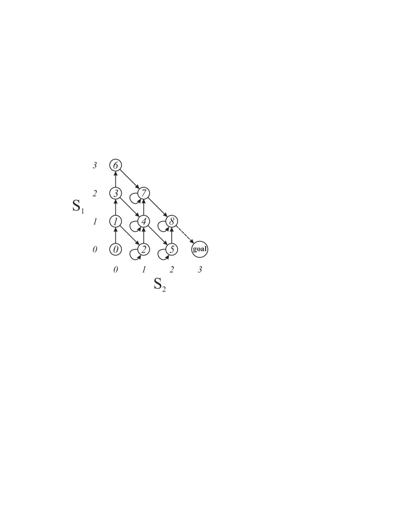
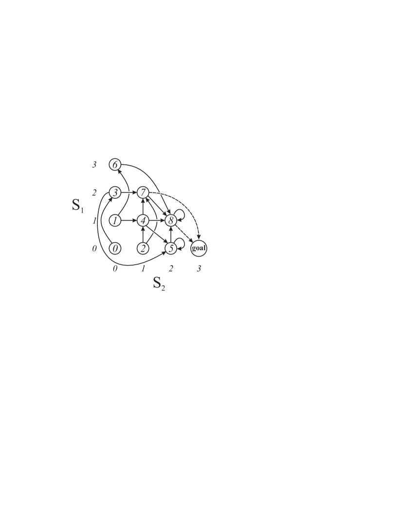
$\begin{array}[]{llcccccccccrr}&&(0,0)&(0,1)&(1,0)&(0,2)&(1,1)&(2,0)&(0,3)&(1,2)&(2,1)\\ &&\downarrow&\downarrow&\downarrow&\downarrow&\downarrow&\downarrow&\downarrow&\downarrow&\downarrow\\ \\ &\hbox{\multirowsetup$\left(\rule{0.0pt}{56.9055pt}\right.$}&0&0&0&0&0&0&0&0&0&\hbox{\multirowsetup$\left.\rule{0.0pt}{56.9055pt}\right)$}&\rightarrow(0,0)\\ &&1&0&0&0&0&0&0&0&0&&\rightarrow(0,1)\\ &&0&\nicefrac{{1}}{{3}}&\nicefrac{{1}}{{3}}&0&0&0&0&0&0&&\rightarrow(1,0)\\ &&0&\nicefrac{{2}}{{3}}&0&0&0&0&0&0&0&&\rightarrow(0,2)\\ T=&&0&0&\nicefrac{{2}}{{3}}&\nicefrac{{2}}{{3}}&\nicefrac{{1}}{{3}}&0&0&0&0&&\rightarrow(1,1)\\ &&0&0&0&0&\nicefrac{{1}}{{3}}&\nicefrac{{2}}{{3}}&0&0&0&&\rightarrow(2,0)\\ &&0&0&0&\nicefrac{{1}}{{3}}&0&0&0&0&0&&\rightarrow(0,3)\\ &&0&0&0&0&\nicefrac{{1}}{{3}}&0&1&\nicefrac{{1}}{{3}}&0&&\rightarrow(1,2)\\ &&0&0&0&0&0&\nicefrac{{1}}{{3}}&0&\nicefrac{{2}}{{3}}&\nicefrac{{2}}{{3}}&&\rightarrow(2,1)\end{array}$

Figure 2: State embedding and transitions matrix for $P=2$, $M=3$, $L=1$.

For $P=2$, $M=3$ and $L=2$, Figure 3-left shows how the two-dimensional states different from goalare mapped into the integers $\{0,1,2,3,4,5,6,7,8\}$ along with the feasible transitions between the resulting integer states.

Probabilities for those transitions with the exception of the dashed ones are reported in Figure 3-right in the form of the transition matrix $T$.

$\begin{array}[]{llcccccccccrr}&&(0,0)&(0,1)&(1,0)&(0,2)&(1,1)&(2,0)&(0,3)&(1,2)&(2,1)\\ &&\downarrow&\downarrow&\downarrow&\downarrow&\downarrow&\downarrow&\downarrow&\downarrow&\downarrow\\ \\ &\hbox{\multirowsetup$\left(\rule{0.0pt}{56.9055pt}\right.$}&0&0&0&0&0&0&0&0&0&\hbox{\multirowsetup$\left.\rule{0.0pt}{56.9055pt}\right)$}&\rightarrow(0,0)\\ &&0&0&0&0&0&0&0&0&0&&\rightarrow(0,1)\\ &&0&0&0&0&0&0&0&0&0&&\rightarrow(1,0)\\ &&1&0&0&0&0&0&0&0&0&&\rightarrow(0,2)\\ T=&&0&\nicefrac{{2}}{{3}}&\nicefrac{{2}}{{3}}&0&0&0&0&0&0&&\rightarrow(1,1)\\ &&0&0&0&\nicefrac{{1}}{{3}}&\nicefrac{{1}}{{3}}&\nicefrac{{1}}{{3}}&0&0&0&&\rightarrow(2,0)\\ &&0&\nicefrac{{1}}{{3}}&0&0&0&0&0&0&0&&\rightarrow(0,3)\\ &&0&0&\nicefrac{{1}}{{3}}&\nicefrac{{2}}{{3}}&\nicefrac{{1}}{{3}}&0&0&0&0&&\rightarrow(1,2)\\ &&0&0&0&0&\nicefrac{{1}}{{3}}&\nicefrac{{2}}{{3}}&1&\nicefrac{{2}}{{3}}&\nicefrac{{1}}{{3}}&&\rightarrow(2,1)\end{array}$

Figure 3: State embedding and transitions matrix for $P=2$, $M=3$, $L=2$.

Note that all the Markov chains we are dealing with are finite and feature only “forward” transition up to a unique absorbing state that is the final goal. This class of Markov chains is well-understood and the following results are obtained by specializing established methods (see, e.g., [16]).

IV-C Computation of $\mathcal{B}^{{\rm\bf goal}}$

Theorem 7

If the $(\mu_{P}(M)-1)\times(\mu_{P}(M)-1)$ matrix $T$ is such that

$$T_{Q_{P}(S^{\prime\prime}),Q_{P}(S^{\prime})}=\phi(S^{\prime\prime},S^{\prime})\binom{M}{L}^{-1}\prod_{k=0}^{P}\binom{S^{\prime}_{k}}{W_{k}(S^{\prime\prime}-S^{\prime})}$$

and the numbers $\tau_{j}$ are defined as

$$\tau_{j}=\begin{cases}\displaystyle 1&\text{if $j=0$}\\ \displaystyle\frac{1}{1-T_{j,j}}\sum_{k=0}^{j-1}T_{j,k}\tau_{k}&\text{if $j=1,\dots,\mu_{P}(M)-2$}\end{cases}$$ (6)

then

$$\mathcal{B}^{{\rm\bf goal}}=\sum_{j=0}^{\mu_{P}(M)-2}\tau_{j}$$

Proof:

If $\bar{n}$ is such that $S(\bar{n})={\rm\bf goal}$ then

$$\mathcal{B}^{{\rm\bf goal}}=\mathbb{E}[\bar{n}]=\sum_{n=0}^{\infty}\Pr\{\bar{n}>n\}$$

The path is straightforward. At the beginning, no player has a coupon, i.e., the system is in the state $S(0)=(0,0,\dots,0,M)$ with probability 1. Since $Q_{P}(0,\dots,0)=0$ we have $p(0)=\begin{pmatrix}1&0&\dots&0\end{pmatrix}^{\top}=v$, where the column vector $v$ remains implicitly defined.

Starting from this initial condition, the system evolves at each burst and, after $n$ bursts, is characterized by the first-order probabilities $p(n)=T^{n}v$.

The probability that $\bar{n}>n$ is the probability that, after $n$ bursts, the system is in any state but goal, i.e., $\Pr\{\bar{n}>n\}=\sum_{j=0}^{\mu_{P}(M)-2}p_{j}(n)=\begin{pmatrix}1&\dots&1\end{pmatrix}p(n)=up(n)$, where the row vector $u$ remains implicitly defined.

$$\mathcal{B}^{{\rm\bf goal}}=\sum_{n=0}^{\infty}uT^{n}v=u\left(I-T\right)^{-1}v$$ (7)

where $I$ is the identity matrix. Note that the inversion of $(I-T)$ is possible since $T$ is lower triangular and thus exhibits its eigenvalues on the diagonal, and since such eigenvalues (that are the probabilities that none of the $L$ coupons of the incoming lot can be assigned to any player) are less than one if the common goals has not been achieved yet.

Note finally that $I-T$ is also lower triangular. Hence, the above expression can be easily expanded component-wise to realize that, by defining the sequence of $\tau_{j}$ as in (6), we get the thesis. ∎

In Figure 4 we report $\frac{\mathcal{B}^{{\rm\bf goal}}L}{P}$ against $M$ for different values of $P$ and $L$. The adoption of a normalized quantity that measures performance in terms of the average number of coupons received directly by each player allows to compare different configurations.

Besides the general and intuitive trend increasing with $M$, the plots reveal two causes of improvement (i.e., decrease of $\mathcal{B}^{{\rm\bf goal}}$).

The first is the availability of lots with $L>1$. This introduces a correlation between coupon appearance that benefits the collection since it reduces the number of duplicates.

The second is the cooperation between players (i.e., the fact that $P>1$) that introduces additional sources of coupons (the other $P-1$ players) that may contribute to the completion of the collection.

Note how this second effect is, in this plot, much more evident than the first, to the extent that the case $L=1$ is always a very good upper bound on $\mathcal{B}^{{\rm\bf goal}}$ computed for other values of $L$.

Actually, this is due to the fact that, for most of the plotted configurations, $\frac{L}{M}\ll 1$ thus reducing the effect of coupon correlation in lots.

\psfragscanon\psfrag{EBgoal}{$\frac{\mathcal{B}^{{\rm\bf goal}}L}{P}$}\psfrag{M}[0.8]{$M$}\includegraphics[width=303.53267pt]{Ebgoal1.eps}

Figure 4: Normalized performance by varying $M$ for different $P$ and $L$.

As a final remark, from (6) we get that the computation of the $\tau_{j}$ may greatly benefit from the fact that $T$ is, in general, quite sparse.

In fact, the number of feasible transitions from the generic intermediate state $(S_{P},S_{P-1},\dots,S_{0})$ is equal to the number of ways in which the integer $L$ can be decomposed as the sum of $P$ integers $0\leq R_{l}\leq\min\{L,S_{l}\}$. Regardless of the state, this number can be easily bounded from above disregarding the constraint $R_{l}\leq S_{l}$.

Following the same path that led us to compute the total number of feasible state vectors, we obtain that not more than $\binom{L+P}{P}$ transitions are feasible from each intermediate state.

Since there are $\binom{M+P}{P}-1$ states different from the final goal, the number of non-vanishing terms considered in the computation of the $\tau_{j}$ in (6) is not larger than $\binom{L+P}{P}\left(\binom{M+P}{P}-1\right)$.

IV-D Computation of $\mathcal{B}^{{\rm\bf goal}}$ for $P=1$

As noted before, in this case $\mu_{1}(M)=M+1$ since the state of the system is the degree of filling of the collection of the unique player: from 0 coupons to one coupon for each of $M-1$ labels before achieving goal.

In this case

$$T_{j,k}=\begin{cases}\binom{M}{L}^{-1}\binom{M-k}{j-k}\binom{k}{L-j+k}&\text{if $j-k\leq L$}\\ 0&\text{otherwise}\end{cases}$$

The matrix $T$ can be written as $T=E\Lambda E$ where $\Lambda$ is a diagonal matrix with eigenvalues

$$\Lambda_{j,j}=T_{j,j}=\binom{M}{L}^{-1}\displaystyle\binom{j}{L}$$

for $j=0,\dots,M-1$ and where

$$E_{j,k}=\binom{M-k}{M-j}(-1)^{M-j}$$

for $j,k=0,\dots,M-1$.

The matrix $E$ is independent of $L$ and has the noteworthy property of being lower triangular and such that $E^{-1}=E$ or $EE=I$.

Based on this, we may compute the terms $\tau_{j}$ in (6) that are the entries of the first column of $\left(I-T\right)^{-1}=E(I-\Lambda)^{-1}E$, i.e.

$$\tau_{j} = \sum_{k=0}^{j}E_{j,k}\frac{1}{1-T_{k,k}}E_{k,0}$$

$$= \sum_{k=0}^{j}\binom{M-k}{M-j}(-1)^{M-j}\frac{\binom{M}{L}}{\binom{M}{L}-\binom{k}{L}}\binom{M}{M-k}(-1)^{M-k}$$

$$= \binom{M}{L}\binom{M}{j}\sum_{k=0}^{j}\binom{j}{k}\frac{(-1)^{j+k}}{\binom{M}{L}-\binom{k}{L}}$$

Plugging this into (7) we get

$$\mathcal{B}^{{\rm\bf goal}}=$$

$$= \binom{M}{L}\sum_{j=0}^{M-1}\binom{M}{j}\sum_{k=0}^{j}\binom{j}{k}\frac{(-1)^{j+k}}{\binom{M}{L}-\binom{k}{L}}$$

$$= \binom{M}{L}\sum_{k=0}^{M-1}\frac{1}{\binom{M}{L}-\binom{k}{L}}\sum_{j=k}^{M-1}\binom{M}{j}\binom{j}{k}(-1)^{j+k}$$

$$= \binom{M}{L}\sum_{k=0}^{M-1}\frac{(-1)^{k+M-1}}{\binom{M}{L}-\binom{k}{L}}\binom{M}{k}$$

This expression is a special case of equation (5) in [3] for equally probable subsets of $L$ out of $M$ labels.

Moreover, in the special case $L=1$, $\tau_{j}$ turns out to be $\tau_{j}=\frac{M}{M-j}$ thus reproducing the classical $\mathcal{B}^{{\rm\bf goal}}=M\sum_{j=1}^{M}j^{-1}$ whose $M\log M$ asymptotic trend is well-known.

IV-E Computation of $\mathcal{B}^{{\rm\bf first}}$ for $L=1$

The computation of this quantity hinges on counting how many coupon assignments are subsumed by each state $S$ and distinguishing in how many of them at least one player has finished her collection. This can be done straightforwardly in the $L=1$ case that is the one addressed here.

Assume now that $\bar{n}$ is the number of bursts needed by the first player to complete her collection. As before, the average of this quantity can be written starting from its complementary cumulative distribution function as

$$\mathcal{B}^{{\rm\bf first}}=\mathbb{E}[\bar{n}]=\sum_{n=0}^{\infty}\Pr\{\bar{n}>n\}$$

In this case $\Pr\{\bar{n}>n\}$ is the probability that after $n$ burst no player has completed her collection and we may expand

$$\Pr\{\bar{n}>n\}=\sum_{S^{\prime}\neq{\rm\bf goal}}\Pr\{\bar{n}>n|S(n)=S^{\prime}\}\Pr\{S(n)=S^{\prime}\}$$

Note that $S^{\prime}$ spans all the states with the exception of ${\rm\bf goal}$ since the common goal implies that all players have completed their collections.

To compute $\Pr\{\bar{n}>n|S(n)=S^{\prime}\}$ assume that $S^{\prime}=(S_{P},\dots,S_{0})$. Corresponding to that state, the $\sum_{j=1}^{P}jS_{j}$ coupons that are in the game, may be assigned to the $P$ players in

$$U_{P}(S_{P},\dots,S_{0})=\binom{M}{S_{P},\dots,S_{0}}\prod_{j=0}^{P}\binom{P}{j}^{S_{j}}$$

ways, that are all equally probable.

Among those assignments, there are $V$ in which no player has completed her collection. This number $V$ is the difference between $U$ and number of assignments in which exactly $j$ players have completed their collection, for $j=1,...,P$.

Note now that, if $S_{0}>0$ then no player may have completed her collection. In general, if $S_{j}>0$ then not more than $j$ players may have completed their collection.

Assuming that it is possible, the number of assignments in which exactly $j$ players have completed their collections is the number of choices of $j$ players out of $P$ (i.e., $\binom{P}{j}$) times the number of assignments of the remaining $\sum_{k=1}^{P}kS_{k}-Mj$ coupons to the residual $P-j$ players such that none of them have completed their collections. To count these assignments note that since we drop $j$ players that have a coupon for each possible label, if $S_{k}$ was the number of labels for which $k$-players had a coupon before, now only $k-j$ out of the remaining $P-j$ have a coupon for those labels.

Hence we may recursively write

$$V_{P}(S_{P},\dots,S_{0})=U_{P}(S_{P},\dots,S_{0})+$$

$$\displaystyle\hskip 28.45274pt-\sum_{j=1}^{\max\{k|S_{0}=\dots=S_{k-1}=0\}}\binom{P}{j}V_{P-j}(S_{P},\dots,S_{j})$$

to yield

$$\Pr\{\bar{n}>n|S(n)=S^{\prime}\}=\frac{V_{P}(S^{\prime})}{U_{P}(S^{\prime})}$$

Assuming to align all the above conditioned probabilities in the $(\mu_{P}(M)-1)$-dimensional row vector $\nu$ such that $\nu_{j}=\Pr\{\bar{n}>n|S(n)=Q_{P}^{-1}(j)\}$, a path identical to what was followed for $\mathcal{B}^{{\rm\bf goal}}$ leads to

$$\mathcal{B}^{{\rm\bf first}}=\nu\left(I-T\right)^{-1}v$$

Relying on the previous (6) we may finally write

$$\mathcal{B}^{{\rm\bf first}}=\sum_{j=0}^{\mu_{P}(M)-2}\nu_{j}\tau_{j}$$

\psfragscanon\psfrag{EBs}{$\frac{\mathcal{B}^{{\rm\bf goal}}}{P},\frac{\mathcal{B}^{{\rm\bf this}}}{P},\frac{\mathcal{B}^{{\rm\bf first}}}{P}$}\psfrag{M}[0.8]{$M$}\psfrag{P=4 Bthis}[0.7]{$P=4\,\mathcal{B}^{{\rm\bf this}}$}\psfrag{P=4 Bgoal}[0.7]{$P=4\,\mathcal{B}^{{\rm\bf goal}}$}\psfrag{P=4 Bfirst}[0.7]{$P=4\,\mathcal{B}^{{\rm\bf first}}$}\psfrag{P=2 Bthis}[0.7]{$P=2\,\mathcal{B}^{{\rm\bf this}}$}\psfrag{P=2 Bgoal}[0.7]{$P=2\,\mathcal{B}^{{\rm\bf goal}}$}\psfrag{P=2 Bfirst}[0.7]{$P=2\,\mathcal{B}^{{\rm\bf first}}$}\psfrag{P=1 Bgoal, Bfirst, Bthis}[0.7]{$P=1\,\mathcal{B}^{{\rm\bf goal}},\mathcal{B}^{{\rm\bf this}},\mathcal{B}^{{\rm\bf first}}$}\includegraphics[width=303.53267pt]{EBs.eps}

Figure 5: Global performance compared with performance relevant to eoc games by varying $M$ for different $P$.

IV-F Computation of $\mathcal{B}^{{\rm\bf this}}$ for $L=1$

As before, the derivation hinges on counting how many coupon assignments are subsumed by each state $S$ and distinguishing in how many of them the chosen player has finished her collection. This can be done straightforwardly in the $L=1$ case that is the one addressed here.

Assume now that $\bar{n}$ is the number of bursts needed by a specified player to complete her collection. As before, the average of this new quantity can be written starting from its complementary cumulative distribution function as

$$\mathcal{B}^{{\rm\bf this}}=\mathbb{E}[\bar{n}]=\sum_{n=0}^{\infty}\Pr\{\bar{n}>n\}$$

In this case $\Pr\{\bar{n}>n\}$ is the probability that after $n$ burst the chosen player has not completed her collection and we may expand

$$\Pr\{\bar{n}>n\}=\sum_{S^{\prime}\neq{\rm\bf goal}}\Pr\{\bar{n}>n|S(n)=S^{\prime}\}\Pr\{S(n)=S^{\prime}\}$$

Note that $S^{\prime}$ spans all the states with the exception of ${\rm\bf goal}$ since the common goal implies that all players have completed their collections and that

$$\Pr\{\bar{n}>n|S(n)=S^{\prime}\}=1-\prod_{k=0}^{P}\left(\frac{k}{P}\right)^{S^{\prime}_{k}}$$

Assuming to align all the above conditioned probabilities in the $(\mu_{P}(M)-1)$-dimensional row vector $\xi$ such that $\xi_{j}=\Pr\{\bar{n}>n|S(n)=Q_{P}^{-1}(j)\}$, a path identical to what was followed for $\mathcal{B}^{{\rm\bf goal}}$ leads to

$$\mathcal{B}^{{\rm\bf this}}=\xi\left(I-T\right)^{-1}v$$

Relying on the previous (6) we may finally write

$$\mathcal{B}^{{\rm\bf this}}=\sum_{j=0}^{\mu_{P}(M)-2}\xi_{j}\tau_{j}$$

IV-G Details of performance for $L=1$

In Figure 5 we report $\frac{\mathcal{B}^{{\rm\bf goal}}}{P}$, $\frac{\mathcal{B}^{{\rm\bf this}}}{P}$, and $\frac{\mathcal{B}^{{\rm\bf first}}}{P}$ against $M$ for different values of $P$ and for $L=1$. As before we measure performance in terms of the average number of coupons received directly by each player.

As expected, we always have $\mathcal{B}^{{\rm\bf first}}\leq\mathcal{B}^{{\rm\bf this}}\leq\mathcal{B}^{{\rm\bf goal}}$. For $P=1$, $\mathcal{B}^{{\rm\bf this}}=\mathcal{B}^{{\rm\bf first}}=\mathcal{B}^{{\rm\bf goal}}$, while simple symmetry implies that $\mathcal{B}^{{\rm\bf this}}=(\mathcal{B}^{{\rm\bf first}}+\mathcal{B}^{{\rm\bf goal}})/2$ for $P=2$. For $P=4$ we still have $\mathcal{B}^{{\rm\bf this}}\approx(\mathcal{B}^{{\rm\bf first}}+\mathcal{B}^{{\rm\bf goal}})/2$.

Finally, besides the general and intuitive trend increasing with $M$, the plots reveal that improvement due to cooperation applies to all performance figures.

V Conclusions

This work deals with the statistical characterization of multiplayer coupon collector’s games that are a generalization of classical coupon collector’s games with perspective applications in several Information Technology fields.

What is addressed is the combination of benefits and costs due to the possibility of cooperation between $P$ players by means exchanging of coupons that enter the game in lots each of $L$ different units. The local goal of each player is to complete her collection of $M$ distinct coupons. The global goal is the completion of all collections.

Such an exchange process is regulated by a protocol entailing offer, request and transfer phases. Two playing mechanisms are analyzed: one in which players who complete their collection exit the game (eoc games), and one in which they remain active and contribute to the overall exchanging (coc games).

The average cost of offer ($\mathcal{C}^{\rm off}$), request ($\mathcal{C}^{\rm req}$) and transfer ($\mathcal{C}^{\rm tra}$) phases is computed in analytical terms all yielding very simple closed form expressions. The quantities $\mathcal{C}^{\rm req}$ and $\mathcal{C}^{\rm tra}$ turn out to be independent of $L$ and of the statistics of lot drawing.

Costs are larger for coc games than for eoc ones.

As far as performance is concerned, an analytical form is given for the average number of activity bursts needed by the first player to complete her collection ($\mathcal{B}^{{\rm\bf first}}$), a chosen player to complete the collection ($\mathcal{B}^{{\rm\bf this}}$) and by all players to complete their collections ($\mathcal{B}^{{\rm\bf goal}}$).

In this case, the equivalence between coc and eoc games is proved as far as $\mathcal{B}^{{\rm\bf first}}$ and $\mathcal{B}^{{\rm\bf goal}}$ are concerned, and when $L=1$ for $\mathcal{B}^{{\rm\bf this}}$. Computations of this merit figures quantifies the effectiveness of cooperation under different points of view.

References

- [1] B. Rosén, “On the Coupon Collector’s Waiting Time”, The Annals of Mathematical Statistics, 1970, vol. 41, no. 6, pp. 1951-1969
- [2] V.G. Papanicolaou, G.E. Kokolakis, S. Boneh, “Asymptotics for the random coupon collector problem,” Journal of Computational and Applied Mathematics, vol. 93, no. 2, pp. 95-105, 1998
- [3] I. Adler, S.M. Ross, “The Coupon Subset Collection Problem,” Journal of Applied Probability, Vol. 38, pp. 737-746, 2001
- [4] I. Adler, S. Oren, S.M. Ross, “The Coupon-Collector’s Problem Revisited,” Journal of Applied Probability, Vol. 40, pp. 513-518, 2003
- [5] A. N. Myers, H. S. Wilf, “Some New Aspects of the Coupon Collector’s Problem,” SIAM Journal on Discrete Mathematics, vol. 17, pp. 1 - 17, 2004
- [6] P. Neal, “The generalised coupon collector problem,” Journal of Applied Probability, vol. 45, pp. 621-629, 2008
- [7] C. Robert, The Bayesian Choice: from decision theoretic motivations to computational implementation, Springer-Verlag, New York, 2001
- [8] T.A. McCready, N.C. Schwertman, “The Statistical Paleontology of Charles Lyell and the Coupon Problem,” The American Statistician, Vol. 55, No. 4 (Nov., 2001), pp. 272-278
- [9] A. Poon, B. H. Davis, L. Chao, “The Coupon Collector and the Suppressor Mutation,” Genetics, vol. 170(3), pp. 1323 1332, 2005
- [10] M. Ma, “Tabu marking scheme to speedup IP traceback,” Computer Networks, vol. 50, pp. 3536 3549, 2006
- [11] S. R. Kundu, S. Pal, K. Basu, S. K. Das, “An Architectural Framework for Accurate Characterization of Network Traffic,” IEEE Transactions on Parallel and Distributed Systems, vol. 20, pp. 111 - 123, 2009
- [12] P. Flajolet, D. Gardy, L. Thimonier, “Birthday paradox, coupon collectors, caching algorithms and self-organizing search,” Discrete Applied Mathematics, vol. 39, pp. 207-229, 1992
- [13] A. Boneh, M. Hofri, “The coupon-collector problem revisited: a survey of engineering problems and computational methods,” Stochastic Models, vol. 13, pp. 39 - 66, 1997
- [14] E. Bach, “Efficient prediction of Marsaglia-Zaman random number generators,” IEEE Transactions on Information Theory Volume 44, pp. 1253-1257, 1998
- [15] S. Deb, M. Medard, C. Choute, “Algebraic gossip: a network coding approach to optimal multiple rumor mongering,” IEEE/ACM Transactions on Networking, vol. 14, pp. 2486-2507, 2006 Special issue on networking and information theory
- [16] J.G. Kemeny, J.L. Snell, Finite Markov Chains Van Nostrand Publishing Company, 1960