The nonmodular topological phase and phase singularities

Abstract

Generalizing an earlier definition of the noncyclic geometric phase (R.Bhandari, Phys.Lett.A, 157, 221 (1991)), a nonmodular topological phase is defined with reference to a generic time-dependent two-slit interference experiment involving particles with N internal states in which the internal state of both the beams undergoes unitary evolution. A simple proof of the shorter geodesic rule for closure of the open path is presented and several useful new insights into the behaviour of the dynamical and geometrical components of the phase shift presented. An effective hamiltonian interpretation of the observable phase shifts is also presented.

	19/13, 1st Main Road,
	Jayamahal Extension,
	Bangalore 560 046, India.
	email: rajbhand@yahoo.com
	phone: 91-80-23333658

Keywords: polarization, interference, geometric phase, topological phase, Berry’s phase

1 Introduction

Study of interference of particles with internal degrees of freedom e.g. a photon with its two polarization states and a neutron with its two spin-1/2 states has been of interest since long. The famous $4\pi$ spinor symmetry experiments with unpolarized neutrons of Rauch et al. [1] and Werner et al. [2] are some notable early examples. In optics, the Young’s double slit experiment of Pescetti [3] with polarized light and its interpretation in terms of the measurement problem in quantum mechanics is another interesting early example.

The overall phase of the state of an evolving quantum system with N internal states is nontrivial when a possibility of interference of the state with a copy of the unevolved state (produced with the use of a beamsplitter), or with a copy which has evolved differently, exists. The simplest example would be a beam of neutrons, with its two spin states, passing through a box containing an arbitrarily oriented magnetic field and interfering with a part of the beam which has either travelled through free space or through a box contining a different magnetic field. As is now widely recognized, the first definition of a phase difference between beams in two different internal states in such a system was given by Pancharatnam in the context of the two-state system of polarization of light. Pancharatnam made two important contributions to the physics of the phase [4]. Firstly he proposed that the phase difference between two waves in different polarization states is the phase that must be introduced so that their superposition yields maximum intensity. Secondly Pancharatnam showed that if two states A and B are in phase by the above definition, A and C are in phase, then B and C have a phase difference equal to half the solid angle subtended at the centre by the geodesic triangle ABC on the sphere representing the states of the two-state system. This constituted the first formulation of the geometric phase. Following the discovery of the geometric phase in the context of adiabatic cyclic quantum evolutions by Berry in 1983 [5], this quantity is sometimes called “Berry phase”. The next step forward in the problem was the work of Aharonov and Anandan [6] who showed that in an evolution where the state evolves cyclically, if a quantity called the dynamical phase which is equal to the time integral of $<H(t)>$; $H(t)$ being the hamiltonian of the system, is subtracted from the total phase, the remainder is independent of the hamiltonian of the system and is the same, modulo $2\pi$, for all evolutions involving the same cyclic path in the state space. For a two-state system they showed that this quantity is equal to half the solid angle subtended by the closed path at the centre of the state sphere i.e. it is a geometric phase .

Cyclic evolutions however form a very small sub-set of the complete set of evolutions in nature. Even if the evolution is cyclic one may wish to consider only a part of the cycle. To define the phase of a state under a noncyclic evolution or for a partial cycle one needs to take recourse to Pancharatnam’s criterion mentioned above. The first attempt to decompose the phase so defined into a dynamical and a geometrical part was made in ref. [7]. The geometric phase for a noncyclic evolution was defined in this work as being equal to the integral of a two-form over the surface enclosed by the closed curve obtained by closing the open curve by “any geodesic arc” connecting the final state to the initial state. For a two-state system this is equal to half the solid angle subtended by the closed surface at the center of the sphere. There are two problems with this definition. Since the definition allows choice of any geodesic arc, if the open curve were closed by the longer geodesic arc connecting the final to the initial state, this definition gives a geometric phase which differs from the correct phase by $\pi$. Secondly, for systems more complicated than the two-state system, the projective Hilbert space is difficult to visualize hence this definition is difficult to use.

Following these developments, the present author, analyzing a gedanken polarization experiment [8], proposed an algebraic definition of the noncyclic geometric phase. It was proposed in [8] that the difference of the total phase as given by the Pancharatnam’s criterion and the dynamical phase as defined by Aharonov and Anandan in [6] be defined as the geometric phase. It was stated that for a two-state system the geometric phase so defined equals half the solid angle of the closed curve obtained by closing the open curve with the shorter geodesic arc connecting the final state with the initial state. In this work, the reference beam was assumed to be in the same state as the initial state incident on the interferometer [9]. It was shown that the variation of the phase of the evolved beam as a function of parameters of the hamiltonian has several counter-intuitive features. In some regions of the parameter space the phase was found to be insensitive to variation in the parameters while in other regions the phase was found to vary sharply and discontinuously in the vicinity of points of singularity in the parameter space exhibiting $\pm\pi$ phase jumps. The shorter geodesic rule was shown to play an important role in understanding the counter-intuitive features. In a series of interference experiments involving polarization states of light [12, 13, 14, 15] these features and the existence of phase singularities were explicitly demonstrated. In [12, 13] it was demonstrated that the total integrated phase shift measured in going around a circuit encircling phase singularities in the parameter space is equal to $2n\pi$ where $n$ is an integer and that it is zero for a circuit not enclosing a singularity. A review of these experiments and related work can be found in [16].

In view of recent interest in optics in noncyclic polarization changes and the Pancharatnam phase [17] we revisit the work first reported in [8] and present a generalization of the considerations in [8] to a scenario where both beams in the interferometer undergo unitary transformations and present a simple proof for the shorter geodesic rule in the more general context. This generalization provides a new degree of freedom to tune the location of the phase singularities in potential applications. We then propose a formal definition of the nonmodular total topological phase, identify its dynamical and geometric components and note that in a cyclic variation of the parameters of the hamiltonian, the dynamical phase change integrates to zero so that the nonmodular total phase change over a cycle is equal to the geometric phase change, each being equal to $2n\pi$ with $n$ being an integer. Using a specific example of an SU(2) transformation in one arm of the interferometer, the parameters of which are varied, while those in the other beam remain fixed, we demonstrate by numerical sumulation discrete transitions between regions where $n$ has different values so that the global slope of the topological phase curve can change abruptly for small changes in a parameter. We then present an effective hamiltonian picture for the interpretation of phase changes in an interferometer with $SU(N)$ elements.

2 The nonmodular topological phase

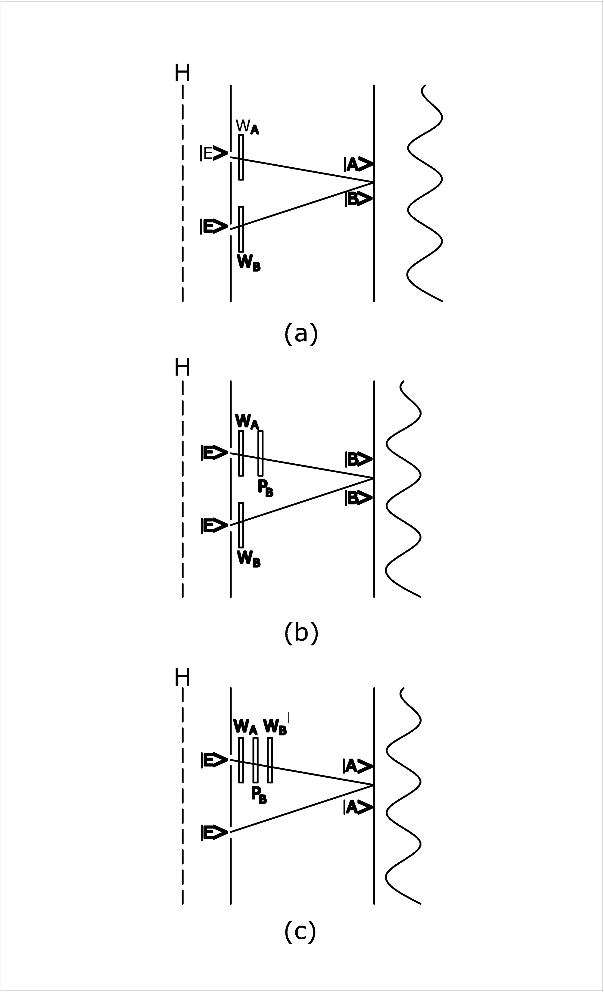
Figure 1: (a) Interference pattern formed on a screen due to interference of two parts of a wavefront H in polarization states $\mid A>$ and $\mid B>$ produced by the action of unitary transformations $W_{A}$ and $W_{B}$ on the initial state $\mid E>$. (b) The phase of the visibility in expt. (a) remains unchanged if a polarizer $P_{B}$ that brings any state to the state $\mid B>$ is placed in front of $W_{A}$ so that both interfering states are $\mid B>$. (c) If $W_{B}$ is removed and a unitary transformation ${W_{B}}^{\dagger}$ is placed in front of the polarizer $P_{B}$ in arm A, the phase of the visibility still remains unaltered.

Consider a version of the standard two-slit interference experiment shown in Fig. 1 in which a coherent plane wave of particles with $N$ internal quantum states, propagating in the $z$-direction is incident on the two slits A and B. Let $|E>$ be the incident wavefunction, represented by a column vector with $N$ complex numbers. Let a box be placed in front of each of the slits such that passage through the box results in a unitary transformation $W_{A}$ or $W_{B}$ being applied to the wavefunction $|E>$, changing its state to $|A>=W_{A}|E>$ or $|B>=W_{B}|E>$. $W_{A}$ and $W_{B}$ are functions of parameters ${\vec{\beta}}_{A}$ and ${\vec{\beta}}_{B}$ which can be varied during the experiment. Let a screen be placed some distance away where the two waves are superposed and the total intensity $I$ recorded at some point P on the screen. The states at P are given by, $|A>e^{i{\chi}_{A}}$ and $|B>e^{i{\chi}_{B}}$, where ${\chi}_{A}$ and ${\chi}_{B}$ are isotropic (state-independent) phases acquired by the wavefunctions $|A>$ and $|B>$ during propagation to the point P. Let $W_{A}=e^{i{\eta}_{A}}U_{A}$ and $W_{B}=e^{i{\eta}_{B}}U_{B}$ where ${\eta}_{A,B}$ are isotropic phase factors associated with $W_{A,B}$ and $U_{A,B}$ are SU(2) transformations. The intensity $I$ at P is given by,

$$I~{}=~{}<A\mid A>+<B\mid B>~{}+~{}2Re[<\tilde{B}\mid\tilde{A}>e^{i({\eta}_{A}-{\eta}_{B})}e^{i({\chi}_{A}-{\chi}_{B})}],$$ (1)

where $\mid\tilde{A}>e^{i{\eta}_{A}}=\mid A>$ and $\mid\tilde{B}>e^{i{\eta}_{B}}=\mid B>$. The fringes on the screen are obtained due to variation of the phase $({\chi}_{A}-{\chi}_{B})$ along the screen. The quantity $<\tilde{B}\mid\tilde{A}>e^{i({\eta}_{A}-{\eta}_{B})}e^{i({\chi}_{A}-{\chi}_{B})}$ is the complex fringe visibility whose phase is the phase difference between the states $|A>$ and $|B>$ and contains a shift in the fringe pattern from its position in the absence of the unitary transformations $W_{A}$ and $W_{B}$, the latter being given by arg $<E\mid E>e^{i({\chi}_{A}-{\chi}_{B})}={\chi}_{A}-{\chi}_{B}$. This shift consists of two parts: (i) the phase of an isotropic, i.e. polarization-independent phase factor $e^{i({\eta}_{A}-{\eta}_{B})}$ and (ii) a polarization-dependent phase shift $\psi={\rm arg}<\tilde{B}\mid\tilde{A}>$. We shall call (ii) the total Pancharatnam phase associated with the evolution. The points in the parameter space at which the magnitude of the fringe visibility $\mid<\tilde{B}\mid\tilde{A}>\mid$ vanishes are the singular points where the contrast in the fringe pattern is zero and its phase is undefined. The singular points could be isolated points or lines or more complicated surfaces in the parameter space. The phase shift $\psi$ is determined modulo $2\pi$. However if small changes in parameters ${\beta}_{A}$ and ${\beta}_{B}$ result in a change $d\psi$ in the phase $\psi$, the integrated phase shift $\int{d\psi}$ is nonmodular. This is the quantity measured in the optical polarization implementations of the above experiment reported in ([12]-[15],[18]).

The physical implementation of the unitary transformations $W_{A}$ and $W_{B}$ will depend upon the nature of the particle used in the interference experiment. For polarization states of light waves, these would typically be a birefringence, possibly variable, distributed along the length of the box represented by the variable $s$. In case of spin-1/2 states of neutrons or atoms these could be a magnetic field distribution, again possibly variable, along the length of the box. An infinitesimal unitary transformation in going from $s$ to $s+ds$, is given by

$$W_{A,B}(s,s+ds)=1-\frac{i}{\hbar}H_{A,B}(s)ds,$$ (2)

where $H_{A,B}$ (i.e. $H_{A}$ or $H_{B}$) is a hamiltonian function determined by the properties of the medium in the box represented by the parameters ${\beta}_{A,B}$.

The finite unitary transformation $W_{A,B}$ can be formally written as,

$$W_{A,B}=e^{-\frac{i}{\hbar}\int H_{A,B}(s)ds}.$$ (3)

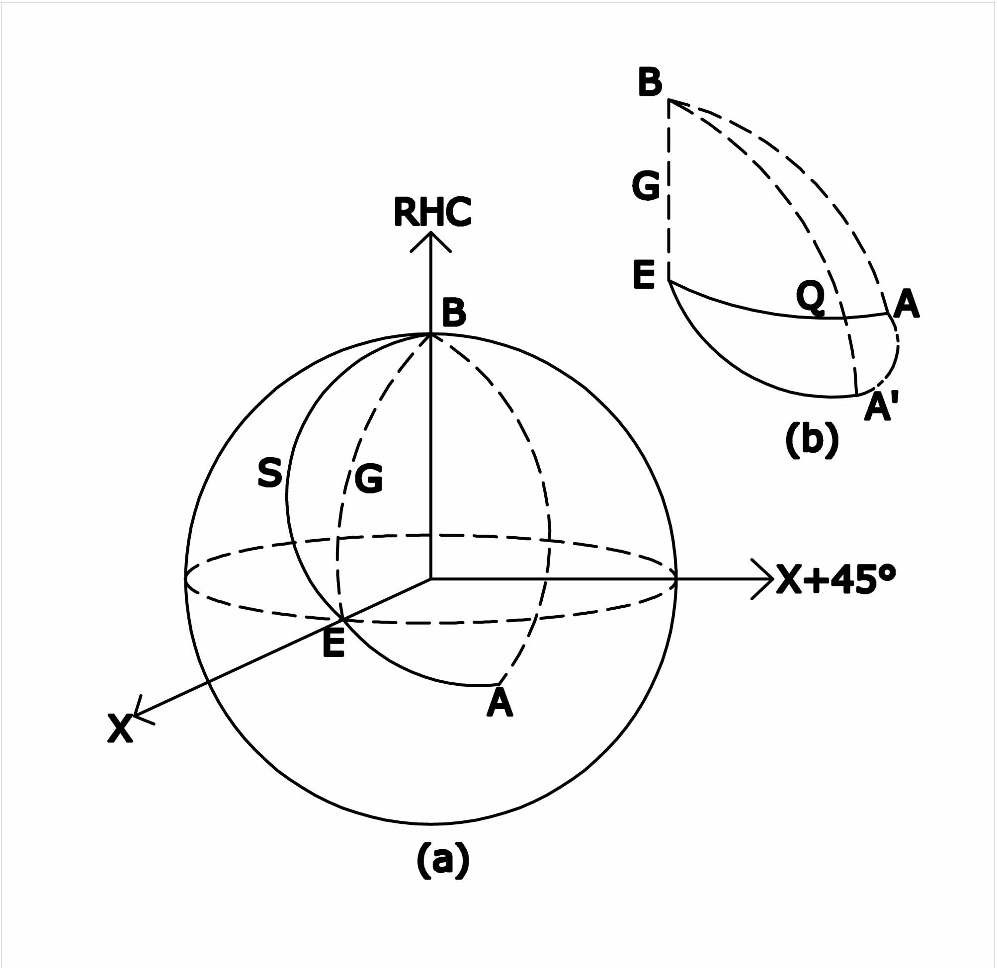
Figure 2: (a) A geometric representation on the Poincaré sphere of transformations of the state of the two-state system of corresponding to the experiment shown in Fig. 1(a). $EA$ is a small circle arc corresponding to the track of the polarization state due to the unitary transformation $W_{A}$ in arm A and $ESB$ is a small circle arc corresponding to the track of the state —B¿ due to $W_{B}$ in arm B. AB is the shorter geodesic arc connecting points A and B and BGE is the shorter geodesic arc connecting points B and E. The geometric phase is equal to half the solid angle subtended by the closed curve $EABSE$ at the centre of the sphere. This can be broken into two parts, the area ESBGE due to the transformation $W_{B}$ and the area EABGE due to the transformation $W_{A}$. (b) The change in the geometric phase as the small circle arc EA moves to EA’ due to change in parameters of the unitary transformation in beam A is given by the difference in the areas EA’BGE and EABGE which can be shown to be equal to the area swept by the moving arc EA plus that swept by the moving geodesic arc AB.

As the particle propagates through the box $A$ or $B$, the internal state of the particle will traverse some path in its state space, shown as $EA$ or $ESB$ in Fig.(2). Following Aharonov and Anandan [6], we can define dynamical phases ${\psi_{d}}^{A}$ and ${\psi_{d}}^{B}$ for these evolutions as,

$${\psi_{d}}^{A}=-\frac{i}{\hbar}\int<A(s)\mid H_{A}(s)\mid A(s)>ds~{}~{}{\rm and}$$ (4)

$${\psi_{d}}^{B}=-\frac{i}{\hbar}\int<B(s)\mid H_{B}(s)\mid B(s)>ds.$$ (5)

We now define the geometric phase for the evolution as :

$$\psi_{g}=\psi-({\psi_{d}}^{A}-{\psi_{d}}^{B}),$$ (6)

where $\psi=<\tilde{B}\mid\tilde{A}>$ is the total Pancharatnam phase for the evolution, defined modulo $2\pi$. For the special case when there is no evolution in arm B, the above definition reduces to the definition given in ref.[8]. For a two-state system the geometric phase $\psi_{g}$ so defined is equal to half the solid angle of the area EABSE in Fig (2) where AB is the shorter geodesic arc joining the points A and B. This is the first main result in this paper.

We now give a simple proof of the above shorter geodesic rule in the context of a two-state system. The proof consists of three steps:

1. Consider the two interference experiments shown in Figs. 1(a) and 1(b). In 1(a) the two interfering beams are in different states A and B. In 1(b) a polarizer $P_{B}$ that projects any state on state B is placed after the unitary transformation $W_{A}$ so that the two interfering beams are in the same state B. It is easy to show that the phase of the visibility in the two experiments is always the same. It is also well known that the action of the polarizer is to bring the state A to the state B along the shorter geodesic arc connecting A to B.

2. Now remove the unitary transformation $W_{B}$ in front of slit B and place a unitary transformation ${W_{B}}^{\dagger}$ in front of the polarizer $P_{B}$ of experiment 1(b). This is shown in Fig.1(c). It is again easy to see that the phase of the visibility in expts. 1(b) and 1(c) is always the same.

3. Since the expt. of Fig.1(c) corresponds to a cyclic evolution of the state in arm A, one can use the decomposition of Aharonov and Anandan [6] to the closed path EABSE for which the dynamical phase is $({\psi_{d}}^{A}-{\psi_{d}}^{B})$. It follows that $\psi_{g}$ given by Eq.( 6) is equal to half the solid angle of the area enclosed by the curve EABSE.

It is conceptually simpler if the evolution in the interferometer were looked upon as a two-step process, first, in the interferometer free from SU(2) evolution, the transformation $W_{B}$ is introduced in arm B and second, the transformation $W_{A}$ is introduced in arm A. The first stage is represented by the circuit ESBGE in Fig.2(a) and the geometric phase acquired by beam B equals half the solid angle of the area ESBGE. The geometric phase acquired by beam A in the second stage of the evolution must therefore be equal to half the solid angle of the area EABGE if the total geometric phase difference for the total evolution has to add up the value stated above. We therefore have the following very useful general result: If the reference beam in the interferometer is in state B (doesn’t matter how it gets there) and in the measurement beam the state evolves from E to A along the curve EA then the geometric phase acquired by beam A is equal to half the solid angle of the closed curve EABGE where AB is the shorter geodesic arc between A and B and BGE is the shorter geodesic arc between B and E. This is our second main result in this paper.

The relation between the geometric phase so defined and the more familiar quantities formulated by Berry [5] and by Aharonov and Anandan [6] can be illustrated by the following example. Let a slab of a cholesteric liquid crystal with its helical axis along the direction of propagation be placed in the path of the beam. Let each layer in the crystal, in addition to linear birefringence, have some optical activity. The propagation of polarized light through such a medium is equivalent to the evolution the spin state of a spin-1/2 particle under the action of a rotating magnetic field, the field making a constant angle $\theta$ with the axis of rotation of the field (ref. [16], p.48). It is well known that under such a hamiltonian, an arbitrary state does not undergo cyclic evolution but a special pair of orthogonal states do [19]. The Aharonov- Anandan phase relates only to the special pair of cyclic states. Berry’s phase is a further special case when the rotation of the state on the state sphere due to birefringence of a single layer is large compared to the rotation of the birefringence axis from one layer to the next (adiabatic limit). For all states other than the cyclic states one needs the definition given by Eqn. (6).

We now introduce the nonmodular phase. For small changes in the parameters ${\vec{\beta_{A}}}$ , the phase changes $d\psi$, $d{\psi_{d}}^{(A,B)}$ and $d\psi_{g}$ are related by,

$$d\psi=d{\psi_{d}}^{A}-d{\psi_{d}}^{B}+d\psi_{g}.$$ (7)

For finite changes in the parameters ${\vec{\beta_{A}}}$ , we therefore have

$$\int d\psi=\int d{\psi_{d}}^{A}-\int d{\psi_{d}}^{B}+\int d\psi_{g}.$$ (8)

The structure of Eqs.(4) and (5) makes it fairly obvious that for any cyclic change in the parameters ${\vec{\beta_{A}}}$,

$$\int d{\psi_{d}}^{A}=\int d{\psi_{d}}^{B}=0.$$ (9)

Eq. (9) implies that if one of the parameters ${\vec{\beta}_{A,B}}$ is an angle variable, ${\psi_{d}}^{A,B}$ must be a periodic function of this variable. Now since a cyclic change in the parameters ${\vec{\beta}_{A,B}}$ must leave the fringe pattern unchanged, Eqs. (8) and (9) lead to the result

$$\int d{\psi}_{g}=\int d\psi=\pm 2n\pi,$$ (10)

where $n$ is an integer. By a cyclic change we mean that at the end of the change the box $W_{A}$ is physically identical to what it was before the change. Eq. (10) is the third main result in this paper. An example of a cyclic change is rotation in space through $2n\pi$ of any of the objects used to make the unitary transformation $W$ or if the object has $m$-fold symmetry about some axis, rotation through $2n\pi/m$ about that axis. In case of the polarization experiments referred above, the objects used to make the unitary transformations $W_{A}$ are quarterwave and halfwave retarders which have a two-fold symmetry about the beam axis and the parameters ${\vec{\beta_{A}}}$ are angles of rotation of these optical elements about the beam axis. In this case therefore Eqs. (9) and (10) are true for rotations through $n\pi$ of any one or more of these optical elements. For example in the experiment of ref. [18], rotation of a halfwave retarder about the beam axis through an angle $n\pi$ yields a total phase change equal to $2n\pi$. A closed cycle in the space of parameters ${\vec{\beta_{A}}}$, where the net rotation of each optical element is zero, is a particularly interesting case where the Eqs. (9) and (10) are true. For example in the experiments reported in [12, 13] a closed circuit enclosing several phase singularities in the parameter space yielded a total phase change equal to $2\pi\Sigma_{k}n_{k}$ where $n_{k}$ is $+1$ or $-1$ depending on the sign of the $k$ th singularity. Eqns. (9) and (10) then imply that these phase changes are geometric.

A geometric picture for the nonmodular geometric phase shift would be as follows. Consider a typical interference situation where the reference beam has been brought to the state B somehow and one is interested in the phase shift as the parameters in beam A are varied. B can be any state on the sphere although in Fig. 2 it has been chosen to be the right circularly polarized state to be consistent with the specific example discussed in the next section. The arc $EA$ is a small circle traced by the state of beam A during passage through some SU(2) element placed in the beam. As stated above the geometric phase is equal to half the solid angle subtended by the closed curve $EABGE$ at the centre of the sphere, where $AB$ is the shorter geodesic arc joining the points $A$ and $B$ and $BGE$ is the shorter geodesic arc joining $B$ and $E$. The nonmodular geometric phase shift is the integrated change in the shaded area in Fig. 2a as the arc EA undergoes changes due to changes in the parameters of $W_{A}$. With the help of Fig. 2b which shows the evolution of the arc $EA$ to the arc $EA^{\prime}$ due to changes in the parameters in beam A the swept area $S$ can be calculated as:

$$S=EA^{\prime}BGE-EABGE=(EA^{\prime}QE+EQBGE)-(EQBGE+QABQ)$$

$$=EA^{\prime}QE-QABQ=(EA^{\prime}AE-A^{\prime}AQA^{\prime})-QABQ=EA^{\prime}AE-BA^{\prime}AB$$

$$=EA^{\prime}AE+A^{\prime}BAA^{\prime}=~{}{\rm Area~{}swept~{}by~{}the~{}moving~{}arc~{}}EA+~{}~{}~{}~{}~{}~{}~{}~{}~{}~{}~{}~{}~{}$$

$${\rm Area~{}swept~{}by~{}the~{}moving~{}geodesic~{}arc}~{}AB.~{}~{}~{}~{}~{}~{}~{}~{}~{}~{}~{}~{}~{}$$ (11)

As explained in [8], the phase jumps are understood as a sudden change in the area swept on the sphere by $AB$ due to a sudden switch of the shorter geodesic arc near a point of singularity where the two interfering states are orthogonal. In many simple examples, the truth of Eq. (10), hence of Eq. (9) can be verified in terms of this geometric picture.

3 A specific example

Consider an interference experiment with particles with two internal states, say the two polarization states of a photon or the two spin states of a neutron. Let us choose an orthogonal set of circularly polarized states (or $|\pm z>$ states in case of spin-1/2 particles) as the basis states and choose the relative phase between them to be such that the state $(1/\sqrt{2})[|+z>+|-z>]$ corresponds to a linear polarization along the $x$-axis (or to the spin-1/2 state $|x>$). Let a state $|E>$=$(1/\sqrt{2})[|+z>+|-z>]$ be incident on the interferometer. Let the reference beam B be brought to the right circularly polarized state by means of a quarterwave plate or a circular polarizer so that

$$|B>=(1/\sqrt{2})|+z>$$ (12)

Let an SU(2) element corresponding to a rotation through an angle $\delta$ (also called retardation) about an axis in the direction represented by the point $(\theta,\phi)$ on the state sphere be placed in arm A of the interferometer so that

$$W_{A}={\rm cos}(\delta/2)-i{\rm sin}(\delta/2)[\vec{\sigma}.\hat{n}],{\rm where}~{}\hat{n}=({\rm sin}\theta{\rm cos}\phi,{\rm sin}\theta{\rm sin}\phi,{\rm cos}\theta).$$ (13)

The components $\sigma_{x},\sigma_{y}$ and $\sigma_{z}$ of the vector $\vec{\sigma}$ are the three Pauli matrices. The final state $|A>$ after passage of the beam through arm A is given by,

$$|A>=W_{A}|E>$$ (14)

A simple calculation shows that the complex visibility $V$ of the interferometer is given by,

$$V=<B|A>=[{\rm cos}(\delta/2)-{\rm sin}(\delta/2){\rm sin}\theta{\rm sin}\phi]-i{\rm sin}(\delta/2)[{\rm cos}\theta+{\rm sin}\theta{\rm cos}\phi].$$ (15)

If $v$ and $\psi$ represent the amplitude and phase of $V$, these quantities can be separately determined uniquely from the equations

$$v_{r}=v{\rm cos}\psi={\rm cos}(\delta/2)-{\rm sin}(\delta/2){\rm sin}\theta{\rm sin}\phi$$

$$~{}{\rm and}~{}v_{i}=v{\rm sin\psi}=-{\rm sin}(\delta/2)[{\rm cos}\theta+{\rm sin}\theta{\rm cos}\phi]$$

$${\rm so~{}that}~{}~{}{\rm tan}\psi=(v_{i}/v_{r})$$ (16)

Consider now an experiment in which $\delta$ and $\theta$ are held fixed and the SU(2) element is rotated about the beam axis from $0$ to an angle $\phi/2$ so that its azimuth on the state sphere rotates by an angle $\phi$. The nonmodular total phase shift is given by

$$\int d\psi=\int[(v_{r}dv_{i}-v_{i}dv_{r})/({v_{i}}^{2}+{v_{r}}^{2})].$$ (17)

The initial phase shift ${\psi}_{0}$ is obtained by substituting $\phi=0$ in Eqs.(16) and computing the argument using the inverse trigonometric function.

The dynamical phase acquired by the beam in passing through the SU(2) element is given by [6]

$${\psi_{d}}=-(\delta/2){\rm cos}\alpha,$$ (18)

where $\alpha$ is the angular length of the geodesic arc connecting the points $(90^{\circ},0^{\circ})$ and $(\theta,\phi)$ on the sphere, given by,

$${\rm cos}(\alpha/2)=|<90^{\circ},0^{\circ}|\theta,\phi>|$$ (19)

Eqs. (18) and (19) give

$${\psi_{d}}=-(\delta/2){\rm sin}\theta{\rm cos}\phi.$$ (20)

Note that $\psi_{d}$ is a periodic function of the angle variable $\phi$.

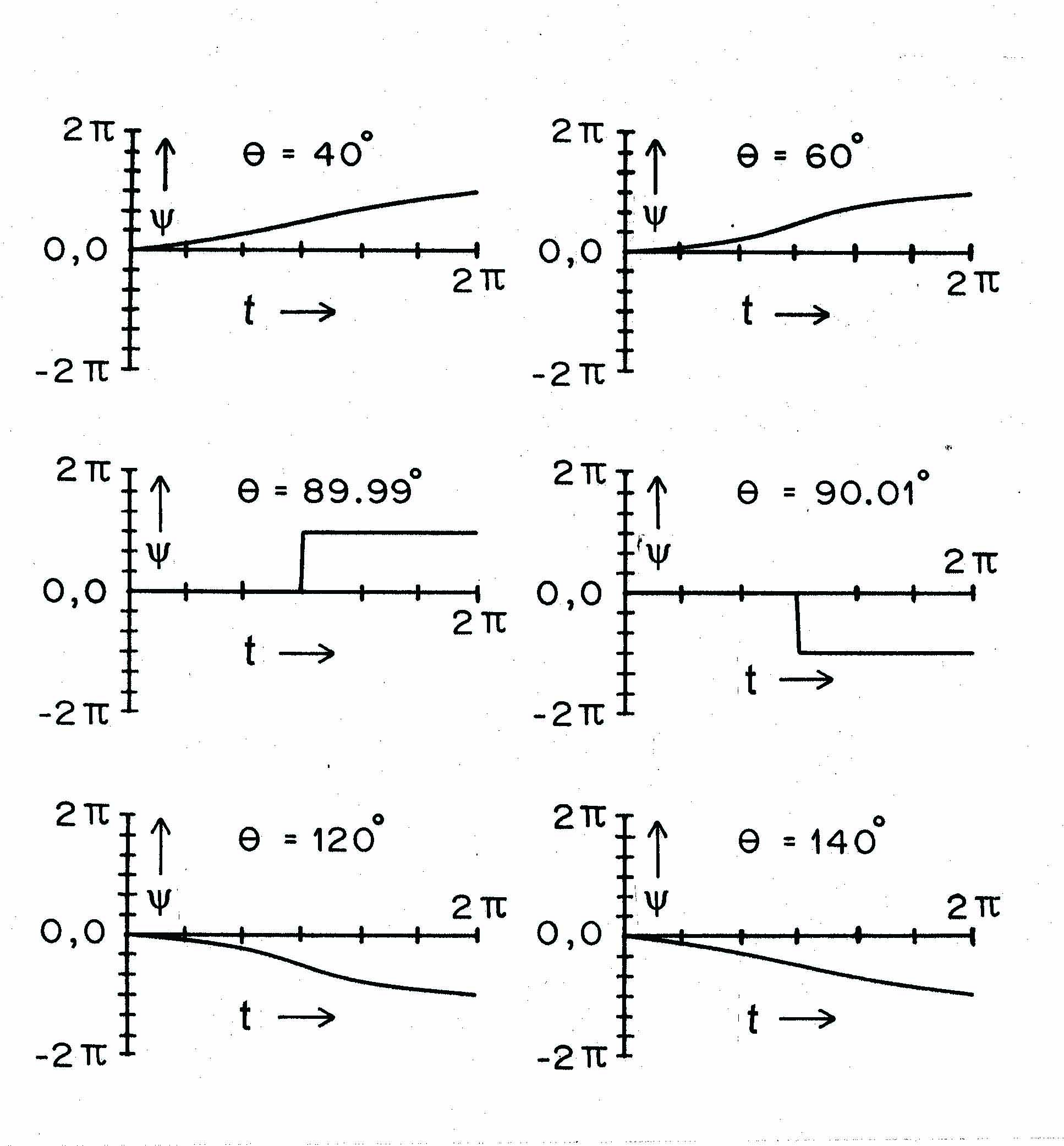
Figure 3: Phase shift $\psi$ as a function of time t when the beam in arm $A$ passes through a magnetic field along $\hat{z}$ varying linearly with time; the reference state for interference being the same as the incident state. The variable $\theta$ represents the polar angle of the incident state on the state sphere and time is expressed as the angle of precession of the spin state. Note the singular behaviour of the phase shift in the vicinity of $\theta=90^{\circ}$ and precession angle $\pi$. For the successive precession periods, the curves repeat themselves with the value at the end of the period as the new zero for the phase.

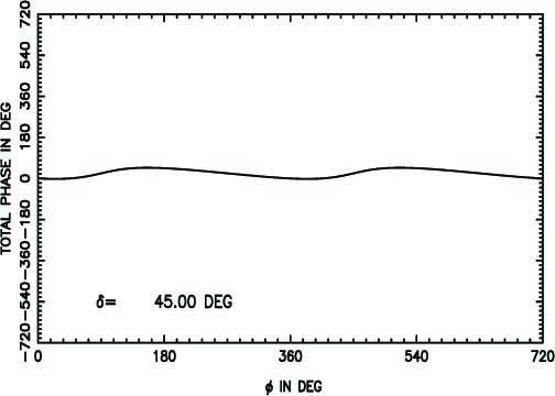
Figure 4: The nonmodular total topological phase as a function of rotation of the SU(2) element on the Poincaré sphere when the retardation of the element is $45^{\circ}$.

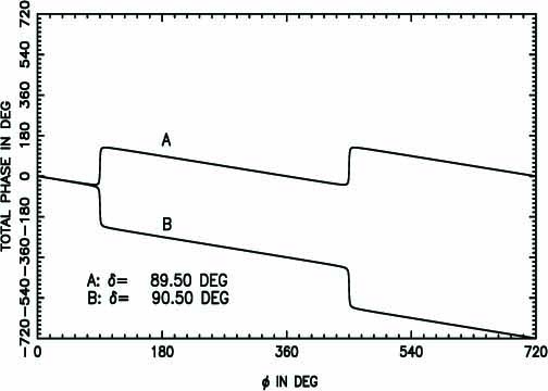
Figure 5: The upper curve shows the nonmodular total topological phase as a function of rotation of the SU(2) element on the Poincaré sphere when the retardation $\delta$ of the element is $89.5^{\circ}$ and the lower curve shows the same quantity when the retardation is $90.5^{\circ}$. Note the discrete $\pm\pi$ jump in the phase when the azimuth $\phi$ is close to $90^{\circ}$ or $450^{\circ}$ resulting in a discrete change in the global slope of the phase curve. The points ($\delta=90^{\circ},\phi=90^{\circ},450^{\circ}$) are phase-singular points.

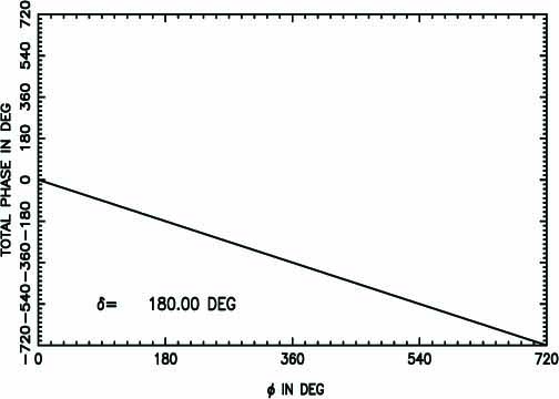
Figure 6: The nonmodular total topological phase as a function of rotation of the SU(2) element on the Poincaré sphere when the retardation of the element is $180^{\circ}$.

We have computed the nonmodular total phase shift $\psi$ which is the sum of ${\psi}_{0}$ and the quantity given by Eq.(17), for $\theta=90^{\circ}$ and various values of $\delta$ as a function of $\phi$. The hamiltonian acting on the beam in this case is exactly the same as that in the second example discussed in the previous section. The angle $\phi$ equals twice the angle of rotation of the SU(2) element about the beam axis. This corresponds to the second example considered in the previous section. Figs. (3-6) show the results. The polar angle $\theta$ of the eigenstate of the SU(2) element is equal to $90^{\circ}$ i.e. it lies on the equator in all the cases. The interesting thing to note is the behaviour of the phase curves in the vicinity of the points $(\delta=90^{\circ},\phi=90^{\circ})$, $(\delta=90^{\circ},\phi=450^{\circ})$ in Fig. 4 and the points $(\delta=270^{\circ},\phi=270^{\circ})$, $(\delta=270^{\circ},\phi=630^{\circ})$ in Fig. 6. These are the points where the two interfering beams are in orthogonal states. The phase jumps by $+\pi$ or $-\pi$ depending on whether $\delta$ is less than or greater than $90^{\circ}$ in case of Fig. 4 and on whether $\delta$ is greater than or less than $270^{\circ}$ in case of Fig. 6. Also note the change in the global slope of the phase curve for a small change in $\delta$ across the value $90^{\circ}$ in Fig. 4 and the value $270^{\circ}$ in Fig. 6. The curve for $\delta=180^{\circ}$ shown in Fig. 5 shows a linear variation of the phase of the beam as a function of rotation of the SU(2) element. This represents a pure frequency shift of the beam equal to twice the rotation frequency of the SU(2) element. A nonmodular phase curve with a nonzero global slope is an unambiguous signature of a topological phase and was first demonstrated in an interference experiment some time ago [18].

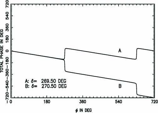
Figure 7: The lower curve shows the nonmodular total topological phase as a function of rotation of the SU(2) element on the Poincaré sphere when the retardation $\delta$ of the element is $269.5^{\circ}$ and the upper curve shows the same quantity when the retardation is $270.5^{\circ}$. Note the discrete $\pm\pi$ jump in the phase when the azimuth $\phi$ is close to $270^{\circ}$ or $630^{\circ}$ resulting in a discrete change in the global slope of the phase curve. The points ($\delta=270^{\circ},\phi=270^{\circ},630^{\circ}$) are phase-singular points.

The dynamical phase as a function of $\phi$, as given by Eq. (20), is shown in Fig. 7 for $\delta=180^{\circ}$. The curves for other values of $\delta$, being exactly similar, with amplitude $\delta/2$, are not shown separately. The global slope of this curve is always zero. The geometric part of the nonmodular topological phase, as defined in [8] is the difference of the total phase as shown in Figs.(3-6) and the corresponding dynamical phase curve. Since the dynamical phase is featureless all the interesting features of the topological phase can be traced to the geometric part of the phase. However since the total phase contains all the interesting features, the curves for the geometric phase are not displayed separately.

4 The effective hamiltonian picture

The time evolution of the state of the beam at the point of interference can be described in terms of an effective hamiltonian $H_{eff}(t)$ as follows.

Let us assume that $W_{A}=W(t)$ where the time variation of $W(t)$ comes from time variation of its parameters $\vec{\beta}$. If the incident state is $\mid E(t)=\mid E(0)>$, the state $\mid A(t)>$ after the SU(2) transformations is given by,

$$\mid A(t)>~{}=~{}W(t)~{}\mid E(t)>~{}=~{}W(t)~{}\mid E(0)>.$$ (21)

so that,

$$\mid A(0)>~{}=~{}W(0)~{}\mid E(0)>~{}.$$ (22)

Now we can define a time-evolution operator $U(t)$ governing the evolution of $\mid A(t)>$ as,

$$\mid A(t)>~{}=~{}U(t)~{}\mid A(0)>.$$ (23)

From the above equations, it follows that,

$$U(t)~{}=~{}W(t)~{}W^{\dagger}~{}(0).$$ (24)

Eqns. (23) and (24) give,

$$\mid A(t+\delta t)>~{}=~{}U(t+\delta t)~{}U^{\dagger}(t)~{}\mid A(t)>~{}=~{}W(t+\delta t)~{}W^{\dagger}(t)~{}\mid A(t)>.$$ (25)

An effective hamiltonian $H_{eff}$ for the evolution of $\mid A(t)>$ can now be defined by the relation:

$$exp[-(i/\hbar)~{}H_{eff}(t)~{}\delta t]~{}=~{}W(t+\delta t)~{}W^{\dagger}(t)$$ (26)

It follows that

$$1-(i/\hbar)H_{eff}(t)~{}\delta t~{}=~{}W(t+\delta t)~{}W^{\dagger}(t)$$ (27)

This leads to,

$$H_{eff}(t)=i\hbar\dot{W}(t)~{}W^{\dagger}(t)$$ (28)

Now if $W(t)$ is cyclic, i.e. if $W(t+T)=W(t)$, the hamiltonian generated by eqn.(28) leads to a cyclic $U(t)$, i.e. $U(T)=U(0)=\bf{1}$ which in turn implies that all states reproduce after time $T$ along with their phases which must therefore be equal to $2n\pi$. The value of $n$ will also depend on the reference state used for interference. This general recipe is valid for $N$-state systems where $W(t)$ is an SU($N$) matrix and can be used as a recipe to generate hamiltonians under which entire state spaces undergo cyclic evolution.

We illustrate the effective hamiltonian picture with two examples for $N$=2. As the first example, let a monoenergetic beam of spin-1/2 particles propagate through a box with a magnetic field along $\hat{z}$ whose magnitude varies linearly with time. Let the magnitude of the field and the length L of the box be adjusted so that the particles precess through an angle $\delta=at$ during passage through the box. $W(t)$ for this setup is given by,

$$W(t)={\rm cos}(at/2){\bf 1}-i{\rm sin}(at/2){\sigma}_{z}$$ (29)

Use of eqn.(28) then leads to the effective hamiltonian matrix:

$$H_{eff}=(a\hbar/2){\sigma}_{z}$$ (30)

At the point of interference therefore the evolution of the state is like precession in a constant magnetic field. If a beam of spin-1/2 particles with the spin state making an angle $\theta$ with the z-axis is incident on the interferometer and the initial state is taken as the reference state, the measured phase variation as a function of time will be as shown in Fig. 3 with the curves for $\theta=89.99$ and $\theta=90.01$ showing $\pm\pi$ phase jumps at values of $t$ for which the interfering states become orthogonal. Fig. 3 is essentially the same as Fig. 4 of ref.[14]. We note that the sign of the $\pi$- phase jump is measurable and has indeed been measured in [14, 15] where both $+\pi$ and $-\pi$ phase jumps are seen. Some optical interference experiments by other groups [20, 21] in similar contexts have measured phase jumps of only one sign leaving behind the impression that the sign is insignificant. We emphasize that a full description of the singularity requires both $+\pi$ and $-\pi$ phase jumps. A proposal to observe phase singularities in a neutron interferometer experiment was made in [22].

We may also mention in passing that instead of spin-1/2 particles, if a beam of spin-$N$ particles were prepared in an initial state $\mid N,N>$ with the axis of quantization being along $\hat{n}=({\rm sin}\theta,0,{\rm cos}\theta)$ the observed phase curves will be exactly $N$ times those shown in Fig.3 with phase jumps equal to $\pm N\pi$. This nonmodular aspect is directly related to the total spin quantum number $N$ and is clearly physically significant.

As the second example, let a monoenergetic beam of spin-1/2 particles propagate through a box in the z-direction and a rotating magnetic field $\vec{B}=(B{\rm cos}\omega t,B{\rm sin}\omega t,0)$ be applied in the $x,y$ plane. Let the magnitude of the field and the length L of the box be adjusted so that the particles precess through an angle $\delta$ during passage through the box. This example corresponds to the example for which the numerical simulations have been considered in the previous section. $W(t)$ for this setup is given by,

$$W(t)={\rm cos}(\delta/2){\bf 1}-i{\rm sin}(\delta/2)({\rm cos}\omega t{\sigma}_{x}+{\rm sin}\omega t{\sigma}_{y})$$ (31)

Use of eqn.(28) then leads to the hamiltonian matrix:

$$H_{eff}=-\hbar\omega{\rm cos}\eta(\hat{n}.\vec{\sigma}),~{}~{}~{}~{}{\rm where}$$ (32)

$$\eta=(90^{\circ}-\delta/2)$$ (33)

$${\rm and}~{}\hat{n}=({\rm sin}\eta{\rm cos}(\omega t+\pi/2),{\rm sin}\eta{\rm sin}(\omega t+\pi/2),{\rm cos}\eta)$$ (34)

At the point of interference therefore beam A sees an effective rotating magnetic field whose parameters are related to those of the rotating field placed in the path of the beam by Eqs.(32-34). For the special case of $\delta=\pi$, i.e. for a rotating halfwave plate or a “$\pi$-flipper” placed in the path of beam $A$, the equations give a constant effective field along $\hat{z}$ which is intuitively obvious. Eqs.(32-34) imply that for a rotating magnetic field whose magnitude corresponds to a Larmor precession frequency $\omega_{L}$, which makes a constant angle $\eta$ with the z-axis and which rotates about the z-axis with frequency $\omega$, the entire state space undergoes cyclic evolution when the following condition is satisfied by the parameters $\omega_{L},\omega$ and $\eta$:

$$\omega_{L}=2\omega{\rm cos}\eta$$ (35)

As an illustration of the significance of this condition, in the example of the cholesteric liquid crystal discussed earlier, when the parameters of the sample satisfy the condition corresponding to Eq.(35), the sample behaves, with respect to polarization, as a piece of plain glass.

We note that while the total phase shift obtained in both the pictures is obviously the same the decomposition into a dynamical and a geometric phase is different. In the effective hamiltonian picture, the total nonmodular phase shift is given by $\int d\psi(t)$ where

$$\psi(t)={\rm arg}<B\mid U(t)\mid A(0)>,$$ (36)

the dynamical phase is given by Eq.(4) with $H_{A}$ replaced by $H_{eff}$ and the nonmodular geometric phase is given by the area swept by the moving geodesic arc AB alone.

5 Discussion

In this paper we have explored a new dimension of the noncyclic geometric phase acquired by an evolving state namely its dependence on the reference state used for interference. This is like studying the phase of matrix elements of the time evolution operator $U(t)$ other than the diagonal matrix element studied earlier.

We have presented two different ways of understanding nonmodular phase changes in a generic interference setup shown in Fig.1, where the unitary transformation $W_{A}$ is a function of some variables $\vec{\beta}$ which can be varied in time. In the first picture one considers evolution through the sequence of elements whose product is $W_{A}$ at time $t$, computes the total Pancharatnam phase shift, does the same thing at a slightly later time $t+\delta t$ and takes the difference to obtain the observed phase shift for the infinitesimal evolution. This is equal to the sum of (i) change in the dynamical phase shift and (ii) the change in the geometric phase shift which is given by the appropriate areas swept on the sphere. Integration of such phase shifts give the total phase shift for the finite evolution. In the second picture one constructs an effective time varying hamiltonian as seen by the beam at the point of interference and considers the phase shifts acquired by the final state for evolution under the effective hamiltonian. While the total phase shift obtained in the both the pictures is the same, the decomposition into the dynamical and the geometric parts is different .

While the second picture is closer to the usual theoretical treatements, the first picture gives useful insights in cases where the evolution of the parameters in the main beam is cyclic. In such cases the dynamical phase shift $\int d{\psi}_{d}$ for a full period of $\vec{\beta}$ is equal to zero. In other words the nonmodular dynamical phase shift is a periodic function of $\vec{\beta}$ and its global slope is equal to zero. The statements imply that when a beam of particles with $N$ internal states passes through an object which performs a sequence of $U(N)$ transformations on the state, the total nonmodular dynamical phase acquired by the state is defined unambigously for every incident state and is independent of a reference state. It is thus an intrinsic property of the system. The nonmodular total phase shift and therefore the geometric part of the phase shift however need not integrate to zero over a period of $\vec{\beta}$ and can equal $2n\pi$ where $n$ is an integer. These quantities therefore need not be periodic functions of $\vec{\beta}$. Therefore, unlike the dynamical phase, the geometric phase acquired by the state is defined only modulo $2\pi$ and can change by $2N\pi$ under cyclic evolutions of the system, the value of $N$ depending not only on the cycle of parameter changes but also on the reference state with respect to which the phase changes are measured. For two-state systems such changes are determined entirely by the appropriate areas swept on the sphere.

We have presented an example demonstrating that the total phase shift over a cycle of a cyclic parameter is absolutely robust except at singular points in the parameter space where the nonmodular phase shift can make a sudden transition from one value of $n$ to another for a small change in parameter, i.e. can undergo a discrete jump in its global slope. The phase variations can be extremely sharp in the vicinity of these points.

Both the above mentioned properties namely robustness of the global slope of the topological phase shift and the possiblity of discrete transitions from one value of $n$ to another can form the basis of applications perhaps in the area of quantum information. An example of the first kind is the achromatic retarders developed by Pancharatnam [23] for polarized light. Some examples of the second kind have been described in [24] where it is shown that (i) an array of radio antennas phased using topological phase shifters can be made to look in two different directions at two different wavelengths at the same time and (ii) one can make a geometric phase lens which can switch from being convex to being concave with a change of wavelength of light passing through it.

We also wish to note that while the focus in this paper is on unitary transformations, we expect the results to have suitable generalizations to nonunitary transformations. Finally we point out an interesting extension of the Pancharatnam phase criterion to partially polarized waves by Sjöqvist et. al [25]. It was shown in [26] that phase singularities form an important part of the description in this case too.

6 Note added

The author’s attention has been drawn by one of the referees to a paper by Berry [27] that describes the theory of $2n\pi$ phase shifts arising from change in the number of dislocation lines threading an interferometer. This paper makes the very interesting observation that even the isotropic, polarization-independent phase shifts arising from a change in the optical path difference between two beams of an interferometer are topological in one sense. The considerations in [27] however differ from those in the present paper and in our earlier work in the following respects. While in [27] the interferometer configurations corresponding to the different values of $n$ look physically different in that they enclose different number of dislocation lines, in the present paper and in our earlier work the $2n\pi$ phase shifts arising from cyclic variation of parameters in the interferometer beams leave the interferometer physically unchanged. Secondly, while the singularities in Berry’s work reside in physical space, those in our work reside in the space of parameters of the unitary transformations that act on the internal degrees of freedom of the interfering particle, for example polarization in case of the photon.

The relationship of our work with spatial singularities of the electromagnetic field can be further illustrated with the help of the following illustration. Let $\hat{z}$ be the propagation direction. At $z=-\epsilon$, let a screen be placed normal to the beam which is a polarizer that passes the state $|E>$. At $z=o$, let an ”SU(2) screen” be placed which is such that at each point in the $x,y$ plane an element is placed which performs an SU(2) transformation on the fields that pass through that point. At $z=\epsilon$, let a third screen be placed which is a polarizer that passes the state $|B>$. Now let the amplitude and phase of the fields at each point in a plane normal to the beam at $z=2\epsilon$ be examined. There will be points or lines at which the amplitude of the field will be zero. These are the singular points or lines. Now let a phase detector be taken in a closed circuit around an isolated singular point. If the phase detector is such that it integrates phase shifts as it goes along, the total phase shift recorded in one such circuit will be equal to $2n\pi$ where $n$ is the strength of the singularity. Such an experiment is not very convenient to perform. What can easily be done however is to replace $xandy$ with two variable SU(2) parameters in one of the beams of an interferometer such that variation of these parameters results in the same sequence of SU(2) transformations on the polarization state as in the spatial example above. This is what is done in our experiments and the two are equivalent. While the spatial analogy presented above works only for two parameters, in our experiments one can in principle have more than two variable parameters.

7 Acknowledgements

A good part of the work reported in this paper was done during the period the author was employed with the Raman Research Institute, Bangalore. Library support from the institute after the author’s retirement is gratefully acknowledged.

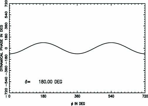
Figure 8: The nonmodular dynamical phase for retardation $180^{\circ}$ as a function of rotation of the SU(2) element on the Poincaré sphere which is equal to half the angle of rotation of the element in real space.

References

- [1] H. Rauch, A.Zeilinger, G.Badurek, A.Wilfing, W.Bauspiess and U.Bonse, “Verification of coherent spinor rotations of fermions”, Phys. Lett. A 54, 425-427 (1975) .
- [2] S.A. Werner, R. Colella, A.W. Overhauser and C.F. Eagen, “Observation of the phase-shift of a neutron due to precession in a magnetic field”, Phys. Rev. Lett. 35 1053-1055 (1975) .
- [3] D. Pescetti, “Interference between elliptically polarized light beams”, Am. J. Phys. 40, 735-740 (1972).
- [4] S. Pancharatnam, “Generalized theory of interference and its applications”, Proc. Indian. Acad. Sci. A44, 247-262 (1956) andCollected works of S. Pancharatnam (Oxford 1975).
- [5] M. V. Berry, Proc. Roy. Soc. London A392, 45 (1984).
- [6] Y. Aharonov and J. Anandan, “Phase change during a cyclic quantum evolution”, Phys. Rev. Lett. 58, 1593-1596 (1987).
- [7] J. Samuel and R. Bhandari, “General setting for Berry’s phase”, Phys. Rev. Lett. 60, 2339-2342 (1988).
- [8] R. Bhandari, “SU(2) phase jumps and geometric phases”, Phys. Lett. A 157, 221-225 (1991).
- [9] The algebraic definition for the noncyclic geometric phase introduced in [8] can be found incorporated in a later, more formal treatment of the subject by Mukunda and Simon [10]. We also refer the theoretically inclined reader to a paper by Pati [11] that deals with the geometric aspects of noncyclic quantum evolution.
- [10] N. Mukunda and R. Simon, “Quantum kinematic approach to the geometric phase”, Ann. Phys. (N.Y.) 228, 205-268 (1993) .
- [11] A.K. Pati, Phys. Rev. A 52, 2576-2584 (1995).
- [12] R. Bhandari, “Observation of Dirac singularities with light polarization - I”, Phys. Lett. A 171, 262-266 (1992).
- [13] R. Bhandari, “Observation of Dirac singularities with light polarization -II” Phys. Lett. A 171, 267-270 (1992).
- [14] R. Bhandari, “4 spinor symmetry-some new observations”, Phys. Lett. A 180, 15-20 (1993).
- [15] R. Bhandari, “Interferometry without beam splitters - a sensitive technique for spinor phases”, Phys. Lett. A 180, 21-24 (1993).
- [16] R. Bhandari, “Polarization of light and topological phases”, Phys. Rep. 281, 1-64 (1997) .
- [17] T. van Dijk, “Geometric interpretation of the Pancharatnam connection and non-cyclic polarization changes”, J. Opt. Soc. Am. A 27, 1972-1976 (2010).
- [18] R. Bhandari, “Observation of non-integrable geometric phase on the Poincaré sphere”, Phys. Lett. A 133, 1-3 (1988).
- [19] S. J. Wang, “Nonadiabatic Berry’s phase for a spin particle in a rotating magnetic field”, Phys. Rev. A 42, 5107-5110 (1990).
- [20] H. Schmitzer, S. Klein and W. Dultz, “Nonlinearity of Pancharatnam’s topological phase”, Phys. Rev. Lett. 71, 1530-1533 (1993).
- [21] Q. Li, L. Gong, Y. Gao and Y. Chen, “Experimental observation of the nonlinearity of the Pancharatnam phase with a Michelson interferometer, Opt. Comm. 169, 17-22 (1999).
- [22] R. Bhandari, “Comment on Experimental Separation of Geometric and Dynamical Phases Using Neutron Interferometry”, arXiv quant-ph/0103134, 1-7 (2001).
- [23] S. Pancharatnam, “Achromatic combinations of birefringent plates-II”, Proc. Indian. Acad. Sci. A 41, 137-144 (1955) and Collected works of S. Pancharatnam (Oxford 1975).
- [24] R. Bhandari, “Phase jumps in a QHQ phase-shifter - some consequences”, Phys. Lett. A 204, 188-192 (1995).
- [25] E. Sjöqvist, A. K. Pati, A. Ekert, J. S. Anandan, M. Ericsson, D.K.L. Oi and V. Vedral, “Geometric phases for mixed states in interferometry”, Phys. Rev. Lett 85, 2845-2849 (2000).
- [26] R. Bhandari, “Singularities of the mixed state phase”, Phys. Rev. Lett 89, 268901-901 (2002).
- [27] M.V. Berry, Proc. R. Soc. A 463, 1697-1711 (2007).