Analytic QCD coupling with no power terms in UV regime

Abstract

We construct models of analytic QCD (i.e.,with the running coupling parameter free of Landau singularities) which address several problems encountered in previous analytic QCD models, among them their incompatibility with the ITEP-OPE philosophy (due to UV power terms) and too low values of the semihadronic $\tau$ decay ratio. The starting point of the approach is the construction of appropriate nonperturbative beta functions.

I Introduction

In the perturbative QCD (pQCD), the running coupling $a_{\rm pt}(Q^{2})\equiv\alpha_{s}(Q^{2})_{\rm pt}/\pi$, as a function of $Q^{2}\equiv-q^{2}$ ($q$ being a typical four-momentum transfer of the considered physical process), has so called Landau singularities at $0<Q^{2}\leq\Lambda^{2}$ ($\Lambda^{2}\sim 10^{-1}\ {\rm GeV}^{2}$), thus not reflecting the analyticity of the space-like observables ${\cal D}(Q^{2})$ for all $Q^{2}\in\mathbb{C}\backslash(-\infty,0]$ dictated by the causality of quantum field theories. As a consequence, the evaluated expressions of such observables in pQCD have wrong analyticity properties and become unreliable at low $|Q^{2}|$. In order to overcome this fundamental problem of pQCD, several attempts have been made to restore the correct analytic (i.e., holomorphic) properties of both the coupling parameter $a(Q^{2})$ and the related evaluated expressions of observables, which all go under the generic name of analytic QCD (anQCD).

Various models of anQCD found in the literature (some of them: Refs. ShS -CV2 ; for reviews and further references see Prosperi:2006hx -Cvetic:2008bn ), among them the most popular minimal analytic (MA) model of Shirkov and Solovtsov ShS , have faced criticism based mainly on one or both of the following points, one being theoretical and the other phenomenological:

1. The analytic running coupling parameter $a(Q^{2})$ differs at large $Q^{2}$ from the ordinary pQCD coupling $a_{\rm pt}(Q^{2})\equiv\alpha_{s}(Q^{2})/\pi$ by power terms $\sim(\Lambda^{2}/Q^{2})^{n}$ or $\sim(\Lambda^{2}/Q^{2})^{n}\ln^{m}(\Lambda^{2}/Q^{2})$ [in MA: by terms $\sim(\Lambda^{2}/Q^{2})^{1}$]. However, these then lead in (inclusive) physical observables to the corresponding power corrections which, nota bene, come from the ultraviolet (UV) regime Cvetic:2007ad . If such observables are calculated within the operator product expansion (OPE) mechanism, it is readily seen that such power terms are in conceptual contradiction with the general OPE philosophy which has been vigorously advocated in particular by the ITEP group Shifman:1978bx (see also, e.g., Ref DMW ) and whose validity is strongly indicated by the success of the related QCD sum rules. This philosophy rests on the assumption that OPE is true in general (not only in the perturbative approach) and that it allows to separate short-range contributions from the long-range ones. And it is only the long-range contributions which should lead to power corrections, reflecting the nonperturbative physics. Thus, there is no space for UV-generated power corrections within the ITEP-OPE philosophy.

2. In the widely used MA model, the prediction for one of the best-measured low-energy QCD observables, namely the strangeless $r_{\tau}$, the decay branching ratio of the $\tau$ lepton into nonstrange hadrons, lies in the region $r_{\tau}\approx 0.14$ Milton:1997mi , significantly below the experimental value $r_{\tau}=0.202\pm 0.004$. It appears that anQCD models in general tend to give too low values of $r_{\tau}$ Geshkenbein:2001mn .

Point (2) (the $r_{\tau}$ problem) can be addressed by introducing additional parameters (Refs. Milton:2001mq ; CV2 ); in MA, these parameters (the quark masses) have to be chosen unusually large Milton:2001mq . On the other hand, point (1) (ITEP-OPE) has not been addressed in a more systematic way in the literature hitherto. Within this letter we try to develop a version of analytic QCD which addresses both problems mentioned above. We base our approach on the assumption that the singularity structure of $a(Q^{2})$ reflects the singularity structure of space-like observables ${\cal D}(Q^{2})$ in a “minimal” way, i.e., dictated by physical principles (causality and unitarity) which means that $a(Q^{2})$ is analytic in the complex $Q^{2}$-plane with the exception of a cut along the negative semiaxis starting at $Q^{2}=-M_{\rm thr}^{2}<0$ (there are no massless hadrons). Specifically, we expect $a(Q^{2})$ to be analytic at $Q^{2}=0$. The method of identifying such an analytic coupling consists in starting with an appropriate ansatz for the related beta function and reconstructing from it the coupling $a(Q^{2})$ by solving the renormalization group equation (RGE). Such an approach (cf. Ref. Raczka ) is natural because ITEP-OPE condition can be implemented in this approach in a very simple way, by requiring that beta function $\beta(a)$ as a function of the coupling $a$ be analytic in point $a=0$, and have there the pQCD Taylor expansion $\beta(a)=-\beta_{0}a^{2}(1+c_{1}a+O(a^{2}))$ where $\beta_{0}$ and $c_{1}=\beta_{1}/\beta_{0}$ are universal. However, having the ITEP-OPE condition easily implemented in this way, it turns out to be very difficult to find a beta function which gives simultaneously an analytic coupling $a(Q^{2})$ (i.e., analytic in the complex $Q^{2}$-plane with the exception of the negative semiaxis) and which gives high enough value $r_{\tau}\approx 0.20$ (i.e., compatible with the experimental measurements). In order to obtain analyticity of $a(Q^{2})$, we are led to restrict ourselves to certain classes of beta functions. However, the obtained values of $r_{\tau}$ turn out to be significantly too low unless the beta functions are further modified in a peculiar, perhaps intriguing, manner.

In this letter, in Sec. II we motivate the first class of beta functions which lead to the analyticity of $a(Q^{2})$ while respecting the ITEP-OPE condition. In Sec. III we modify these beta functions in such a way as to obtain the correct value of $r_{\tau}$ while maintaining the analyticity and the ITEP-OPE condition. Section IV summarizes our results and outlines the prospects of further phenomenological applications of the obtained models.

II Beta function ansätze for ITEP-OPE and analyticity

The renormalization group equation (RGE)

$$Q^{2}\frac{da(Q^{2})}{dQ^{2}}=\beta(a(Q^{2}))\ ,$$ (1)

determines the running coupling $a(Q^{2})$ at (in general complex) $Q^{2}$ once an initial condition $a(Q^{2}_{\rm in})=a_{\rm in}$ is imposed. We will impose the initial condition in the present anQCD versions at the scale $Q^{2}_{\rm in}$ of the $3\to 4$ active quark flavor threshold; we choose $Q^{2}_{\rm in}=(3m_{c})^{2}$ ($\approx 14.5\ {\rm GeV}^{2}$). The value of $a_{\rm in}=a(Q^{2}_{\rm in})$ is obtained as usual in perturbative QCD (pQCD). The analytic coupling we get is valid for $n_{f}=3$ (the three active quarks $u$, $d$ and $s$ being almost massless), and for higher energies the standard pQCD couplings can be used because our versions of anQCD, at such high energies, practically merge with the pQCD due to the ITEP-OPE condition:

$$|a(Q^{2})-a_{\rm pt}(Q^{2})|<(\Lambda^{2}/Q^{2})^{n}$$ (2)

at $Q^{2}\gg\Lambda^{2}(\sim 0.1\ {\rm GeV}^{2})$ for all positive $n$.

More specifically, in the renormalization scheme (RSch) dictated by the expansion of our beta function $\beta(a)$ in powers of $a$ (i.e., the parameters $c_{n}\equiv\beta_{n}/\beta_{0}$, for $n\geq 2$), we will require that our $a(Q^{2})$ at $Q=3m_{c}$ achieves such a value $a((3m_{c})^{2})=a_{\rm in}$ which leads to the value $a(M_{Z}^{2};{\overline{\rm MS}})=0.119/\pi$ once we (exactly) change the RSch at $Q=3m_{c}$ to ${\overline{\rm MS}}$ and run the coupling to $Q=M_{Z}$ with ${\overline{\rm MS}}$ perturbative RGE. The latter running is performed at four-loop level, taking the RGE thresholds $n_{f}=3\mapsto n_{f}=4$ at $Q=3m_{c}$ and $n_{f}=4\mapsto n_{f}=5$ at $Q=3m_{b}$, using the procedure of Ref. CKS with three-loop threshold matching conditions (for two-loop matching conditions, cf. Refs. BW ; RS ; LRV ). We note that the value $a(M_{Z}^{2};{\overline{\rm MS}})\approx 0.119/\pi$ is obtained by application of pQCD evaluations to QCD observables of higher energies ($|Q^{2}|\stackrel{{\scriptstyle>}}{{\sim}}10\ {\rm GeV}^{2}$).

With such a fixing of the initial condition, integration of RGE (1) in the complex $Q^{2}$-plane can be made more transparent by introducing the new complex variable $z=\ln(Q^{2}/\mu^{2}_{\rm in})$, with $\mu_{\rm in}$ being a fixed scale; we chose $\mu_{\rm in}=3m_{c}$. The entire complex $Q^{2}$-plane (the first sheet) then corresponds to the complex $z$ stripe: $-\pi\leq{\rm Im}(z)<+\pi$. The complex $Q^{2}$-plane ${\mathbb{C}}\backslash(-\infty,0]$ where $a(Q^{2})$ has to be analytic corresponds to the complex $z$ stripe $-\pi<{\rm Im}(z)<+\pi$, while the Minkowskian semiaxis $Q^{2}\leq 0$ corresponds to ${\rm Im}z=-\pi$; the point $Q^{2}=0$ corresponds to $z=-\infty$, and $Q^{2}=(3m_{c})^{2}$ to $z=0$. Using the notation $a(Q^{2})\equiv F(z)$, RGE (1) can be rewritten in the form

$$\frac{dF(z)}{dz}=\beta(F(z))\ ,$$ (3)

in the semi-open stripe $-\pi\leq{\rm Im}(z)<+\pi$, and requiring for the analyticity of $a(Q^{2})$ in the $Q^{2}$ sector ${\mathbb{C}}\backslash(-\infty,0]$ equivalently the analyticity of $F(z)$ in the open $z$-stripe $-\pi<{\rm Im}(z)<+\pi$ ($\Rightarrow\partial F/\partial{\overline{z}}=0$). If we write $z=x+iy$, and $F=u+iv$, RGE (3) can be rewritten in term of real functions $u$, $v$ and real variables $x$, $y$

$$\frac{\partial u(x,y)}{\partial x} = {\rm Re}\beta(u+iv)\ ,\quad\frac{\partial v(x,y)}{\partial x}={\rm Im}\beta(u+iv)\ ,$$ (4)

$$\frac{\partial u(x,y)}{\partial y} = -{\rm Im}\beta(u+iv)\ ,\quad\frac{\partial v(x,y)}{\partial y}={\rm Re}\beta(u+iv)\ .$$ (5)

If $\beta(F)$ in (3) is an analytic function of $F$ at $F=0$, then $a(Q^{2})$ fulfills ITEP-OPE condition (2). This will be demonstrated in the following lines by assuming that the ITEP-OPE condition is not fulfiled and showing that consequently $\beta(F)$ must be nonanalytic at $F=0$. If ITEP-OPE condition (2) is not fulfilled, then there exists a positive $n_{0}$ such that

$$\delta a(Q^{2})\equiv a(Q^{2})-a_{\rm pt}(Q^{2})\approx\kappa(\Lambda^{2}/Q^{2})^{n_{0}}$$ (6)

when $Q^{2}\gg\Lambda^{2}$. Due to asymptotic freedom at such large $Q^{2}$, $a_{\rm pt}(Q^{2})$ is

$$a_{\rm pt}(Q^{2})=\frac{1}{\beta_{0}\ln(Q^{2}/\Lambda^{2})}+{\cal O}\left(\ln\ln(Q^{2}/\Lambda^{2})/\ln^{2}(Q^{2}/\Lambda^{2})\right)\ ,$$ (7)

and the power term can be written as

$$(\Lambda^{2}/Q^{2})^{n_{0}}\approx\exp\left(-K/a_{\rm pt}(Q^{2})\right)\ ,$$ (8)

where $K=n_{0}/\beta_{0}$. When we apply $Q^{2}d/dQ^{2}$ to relation (6), and use expression (8), we obtain

$$\beta(a(Q^{2}))-\beta_{\rm pt}(a_{\rm pt}(Q^{2}))\approx-n_{0}\kappa\exp\left(-K/a_{\rm pt}(Q^{2})\right)\ .$$ (9)

Now we can replace $a(Q^{2})$ in the first beta function in Eq. (9) by $a_{\rm pt}(Q^{2})+\kappa\exp(-K/a_{\rm pt}(Q^{2}))$, due to relations (6) and (8), and Taylor-expand the $\beta$-function around $a_{\rm pt}(Q^{2})$ ($\not=0$). This then gives

$$\beta(a_{\rm pt})+\kappa\exp(-K/a_{\rm pt})\frac{d\beta(a)}{da}{\big{|}}_{a=a_{\rm pt}}+{\cal O}\left(\exp(-2K/a_{\rm pt})\right)=\beta_{\rm pt}(a_{\rm pt})-n_{0}\kappa\exp(-K/a_{\rm pt})\ .$$ (10)

Since this relation is valid for small values of $|a_{\rm pt}|$, the derivative $d\beta(a)/da$ at $a=a_{\rm pt}$ on LHS of Eq. (10) is very small (about $-2\beta_{0}a_{\rm pt}$) and can be neglected. This means that Eq. (10) can be rewritten for small values of $a_{\rm pt}=F$ as

$$\beta(F)\approx\beta_{\rm pt}(F)-n_{0}\kappa\exp(-K/F)\ .$$ (11)

While $\beta_{\rm pt}(F)$ is analytic at $F=0$, the term $\exp(-K/F)$ is nonanalytic at $F=0$. Therefore, the non-fulfillement of ITEP-OPE condition (2) implies nonanalyticity of $\beta(F)$ at $F=0$, and this concludes the demonstration.

In addition, since at small $F$ the beta function has to respect pQCD, the following condition must be imposed on it:

$$\beta(F)=-\beta_{0}F^{2}\left[1+c_{1}F+c_{2}F^{2}+\cdots\right]\ ,\$$ (12)

where the parameters $\beta_{0}$ and $c_{1}=\beta_{1}/\beta_{0}$ are universal; at $n_{f}=3$ we have $\beta_{0}=9/4$ and $c_{1}=16/9$.

A high precision implementation of the numerical integration of RGE (4)-(5), e.g., with Mathematica math , for various ansätze of $\beta(F)$ function and respecting pQCD condition (12) and the ITEP-OPE condition [analyticity of $\beta(F)$ in $F=0$] then indicates that it is in general difficult to obtain a result $F(z)$ analytic in the entire open stripe $-\pi<{\rm Im}(z)<+\pi$. In our approach we assume that the analytic coupling $a(Q^{2})$ reflects all the major analyticity aspects of the space-like observables ${\cal D}(Q^{2})$ (such as Adler function, Bjorken sum rules, etc.). This means that our $a(Q^{2})$ is analytic even at the origin $Q^{2}=0$ ($\Leftrightarrow\ z=-\infty$). This condition, in general, implies

$$a(Q^{2})=a_{0}+a_{1}(Q^{2}/\Lambda^{2})+{\cal O}[(Q^{2}/\Lambda^{2})^{2}]\ ,$$ (13)

where $a_{0}=a(Q^{2}=0)=F(z=-\infty)<\infty$. By applying to Eq. (13) the RGE derivative $Q^{2}(d/dQ^{2})$, we can see that the beta function $\beta(a)=\beta(F)$ then has a Taylor expansion around the point $a_{0}$ with the first Taylor coefficient equal to unity

$$\beta(F)=1\times(F-a_{0})+{\cal O}[(F-a_{0})^{2}]\ ,$$ (14)

which can be equivalently expressed as

$$\beta^{\prime}(F)|_{F=a_{0}}=+1\ .$$ (15)

If assuming the analyticity of $a(Q^{2})$ at $Q^{2}=0$ in a more exceptional way $a(Q^{2})=a_{0}+{\cal O}[(Q^{2}/\Lambda^{2})^{n}]$ with $n\geq 2$, this implies the condition $\beta^{\prime}(F)|_{F=a_{0}}=n$; it turns out that in such cases the RGE-solution $F(z)$ has Landau singularities, at ${\rm Im}z=\pm\pi/n$; therefore, we discard such a case.

PQCD condition (12) for the universal parameters $\beta_{0}$ and $c_{1}$, the $Q^{2}=0$ analyticity condition (15), and the ITEP-OPE condition can then be summarized in the following form of the beta functions:

$$\beta(F)=-\beta_{0}F^{2}(1-Y)f(Y)|_{Y\equiv F/a_{0}}\ ,$$ (16)

where function $f(Y)$ is analytic at $Y=0$ (ITEP-OPE) and at $Y=1$ and fulfills the conditions

$$f(Y) = 1+(1+c_{1}a_{0})Y+{\cal O}(Y^{2})\ ,$$ (17)

$$a_{0}\beta_{0}f(1) = 1\ .$$ (18)

Eq. (17) is the pQCD condition (reproduction of the universal $c_{1}$), and Eq. (18) is the $Q^{2}=0$ analyticity condition (15). Under such conditions, and the aforementioned initial condition at $Q^{2}=(3m_{c})^{2}$, it turns out that certain classes of functions $f$, upon RGE integration (3), do lead to analytic coupling $F(z)$. Even more so, the $Q^{2}=0$ analyticity condition leads in general to solutions $F(z)=a(Q^{2})$ which have analyticity even on a certain segment of the negative $Q^{2}$-axis [$\leftrightarrow{\rm Im}(z)=-\pi$]: $-M_{\rm thr}^{2}<Q^{2}\leq 0$ [$\leftrightarrow-\infty<{\rm Re}(z)<x_{\rm thr}$], $M_{\rm thr}$ being a “threshold” mass, i.e., the cut semiaxis in the complex $Q^{2}$-plane is $(-\infty,-M_{\rm thr}^{2}]$.

For example, when $f(Y)$ is a polynomial or a rational (i.e., Padé, meromorphic) function, then there exist certain regions of parameters of these $f(Y)$ functions for which $F(z)$ is analytic ($\leftrightarrow a(Q^{2})$ analytic in the entire complex $Q^{2}$-plane with the exception of the cut semiaxis $(-\infty,-M_{\rm thr}^{2}]$). This can be also checked and seen by analytical integration of RGE (3) in such cases

$$z=G(F)\ ,\quad G(F(z))=\int_{a_{\rm in}}^{F(z)}\frac{d{\widetilde{F}}}{\beta({\widetilde{F}})}\ .$$ (19)

Namely, when $f(Y)$ is a polynomial or rational function, integral in Eq. (19) can be performed explicitly (analytically). From such a solution one can see that a pole ($F=\infty$) is attained on the negative $Q^{2}$ semiaxis (at $Q^{2}=-M_{\rm thr}^{2}<0$, i.e., at $z=x_{\rm thr}-i\pi$), and that other poles and singularities would not appear at least for certain range of values of the free parameters CKV . The $Q^{2}=0$ analyticity condition (18) turns out to be crucial for such a behavior.

However, in this approach we encounter a serious problem: virtually all the choices of the $f(Y)$ functions which fulfill the aforementioned conditions (17)-(18) and whose numerical solution is, at the same time, an analytic function, lead to too low values of the semihadronic $\tau$ decay ratio (with $\triangle S=0$): $r_{\tau}<0.16$, while we need $r_{\tau}\approx 0.20$. The “leading-$\beta_{0}$” (LB) contribution is $r_{\tau}^{(LB)}<0.15$ for various classes of beta functions that we tried; if it is possible to adjust free parameters in the beta function ansätze in order to increase $r_{\tau}^{(LB)}$ beyond values $0.15$, Landau singularities of the obtained $F(z)$ [$=a(Q^{2})$] appear. At first, for all the chosen classes of beta functions, the corrections beyond LB (bLB) to $r_{\tau}$ were very small ($<0.10$), and the value $r_{\tau}\approx 0.20$ could not be achieved (some elements of the $r_{\tau}$ calculation are outlined in the Appendix).

This problem is partly a reflection of the fact that, when the analytization of the coupling eliminates the offending nonphysical cut $0<Q^{2}<\Lambda^{2}$ of $a_{\rm pt}(Q^{2})$, the quantity $r_{\tau}$ tends to decrease because the aforementioned cut gave a positive contribution to $r_{\tau}$ Geshkenbein:2001mn .

III R(tau)-problem: modification of beta function ansätze

Since LB contribution $r_{\tau}^{({\rm LB})}$ cannot be increased further, it appears that the only way to increase the total calculated $r_{\tau}$ is to increase the beyond-the-leading-$\beta_{0}$ (bLB) contributions: NLB, ${\rm N}^{2}{\rm LB}$, etc. A choice of the beta function (16) in our approach fixes also the coefficients $c_{2}$, $c_{3}$, etc., that appear in the power expansion (12) of $\beta(F)$ in powers of $F$. On the other hand, the coefficient $T_{2}$ in the third term (${\rm N}^{2}{\rm LB}$) of the expansion of $r_{\tau}$ beyond the LB [see Eqs. (38) and (41)] contains a term $-c_{2}$; if $c_{2}$ can be made significantly negative ($c_{2}\ll-1$) by a suitable choice of beta function (16), then $T_{2}$ and, consequently, ${\rm N}^{2}{\rm LB}$ term in expansion of $r_{\tau}$ will become significantly positive, increasing thus the evaluated value of $r_{\tau}$ (note that coefficient $T_{1}$ of the second, NLB, term is accidentally small, $T_{1}=1/12$, and independent of beta function). On the other hand, we do not want to reduce as significantly the LB contribution when we increase $T_{2}$; and the universal $c_{1}$ coefficient must remain unchanged during such a modification.

A modification which achieves the aforementioned effects is the following:

$$f_{\rm old}(Y)\mapsto f_{\rm new}(Y) = f_{\rm old}(Y)f_{\rm fact}(Y)\ ,$$ (20)

$$f_{\rm fact}(Y) = \frac{(1+BY^{2})}{(1+(B+K)Y^{2})}\ ,\quad(1\ll K\ll B)\ .$$ (21)

The modification factor $f_{\rm fact}(Y)$ is chosen in such a way ($K\ll B$) that, for most of the values of $Y$, it is close to one. Therefore, it does not change significantly beta function (16). This means that, if before the modification the LB part of $r_{\tau}$ was reasonably large (say, $0.14$-$0.15$), it will not be changed (reduced) very significantly now. PQCD condition (17) will not be modified by such $f_{\rm fact}(Y)$ because it modifies the expansion coefficients of $\beta(F)$ only at order $\sim F^{4}$ (i.e., $c_{2}$) and higher. However, since $1\ll K$, the modification factor $f_{\rm fact}(Y)$ can decrease the value of $c_{2}$ significantly and thus increase significantly the third term in the expansion of $r_{\tau}$. Numerical investigations indicate that this is really so, and that, moreover, Landau singularities are not introduced by such a modification. The latter point can be understood even by analytical (i.e., explicit) integration of the RGE in such a case when $f_{\rm old}$ is a polynomial or a rational function CKV .

The solution, however, comes at a price. The aforementioned modification increases very significantly the absolute values of the higher expansion coefficients $c_{n}$ ($n\geq 4$) of beta function. As a consequence, coefficients $|T_{n}|$ [$\approx c_{n}/(n-1)$] in the expansion become very large when $n\geq 4$. This means that the expansion series for $r_{\tau}$ starts showing signs of divergence after the first four terms. On the other hand, the behavior of the first four terms (including ${\rm N}^{3}{\rm LB}$) indicates reasonable behavior (similar is the behavior of asymptotically divergent perturbation series in pQCD).

The fact that the values of parameters $|c_{2}|$, $|c_{3}|$, etc., are large does not mean that we are working in a “wrong” renormalization scheme (RSch). The specification of the RSch in terms of coefficients $c_{j}=\beta_{j}/\beta_{0}$ ($j\geq 2$) is apparently a perturbative concept, applicable in the regime $|Q^{2}|\gg\Lambda^{2}$. It appears that our beta function $\beta(F)$ not just fixes a certain set of values $c_{j}$ ($j\geq 2$), but it reflects also certain nonperturbative aspects via its set of zeros and poles in the complex $F$-plane. For example, the finite value $a_{0}=a(Q^{2}=0)$ is a zero of the beta function; the function $f_{\rm new}(Y)$ [with $Y=a(Q^{2})/a_{0}=F(z)/a_{0}$] has possibly some zeros and/or poles on the real axis [but not in the interval $Y\in(0,1)$], and it has two zeros and poles on the imaginary axis close to the origin [at $F=\pm iB^{-1/2}$ and $F=\pm i(B+K)^{-1/2}$, respectively]. It appears that, while we might be able to go from one set of values of $c_{j}$’s to another in this framework, we cannot go to the “tame” pQCD schemes such as ${\overline{\rm MS}}$ or ’t Hooft RSch. For example, the ’t Hooft RSch ($c_{2}=c_{3}=\ldots=0$), under the assumption of the ITEP-OPE condition, gives us $\beta(F)=-\beta_{0}F^{2}(1+c_{1}F)$ and the solution in such a case violates analyticity, it has namely a Landau cut Gardi:1998qr ). Thus it cannot be physically equivalent at $Q^{2}\stackrel{{\scriptstyle<}}{{\sim}}\Lambda^{2}$ to RSch’s of our beta functions. The same is true for ${\overline{\rm MS}}$ RSch, at least in its hitherto known truncated form. These considerations lead us to intriguing questions which may be clarified in the future.

Table 1: Input parameter values of the three considered $\beta$-ansätze, and some resulting values of other parameters: $c_{2}$, $c_{3}$ of expansion (12), and $a(Q^{2})$ at $Q=3m_{c}$ and $Q=0$ ($n_{f}=3$ used).

$f_{\rm old}$	input $f_{\rm old}$	input $f_{\rm fact}$	$c_{2}$	$c_{3}$	$x_{\rm thr}$	$a\left((3m_{c})^{2}\right)$	$a(0)$
P30	$w_{1}=1+i0.45$	$K=43.2,B=5000$	-243.6	-250.1	-12.00	0.0545	0.4596
P11	$Y_{\rm pole}=-10.$	$K=7.0,B=4000$	-213.3	-293.9	-6.44	0.0577	0.1995
EE	$y_{1}=0.1,k_{1}=10.,k_{2}=11.$	$K=5.27,B=1000$	$-104.5$	$-322.7$	-5.88	0.0613	0.2370

Table 2: The first four terms in expansion (38) of $r_{\tau}$ and their sum, in the three considered models. In parentheses are the corresponding results for expansion (43). RScl parameter is ${\cal C}=0$; $n_{f}=3$. The last column are variations ($\delta$) of the sums when RScl-parameter ${\cal C}$ increases from $0$ to $\ln(2)$.

$f_{\rm old}$	$r_{\tau}:$ LB (LO)	NLB (NLO)	${\rm N}^{2}{\rm LB}$ (${\rm N}^{2}{\rm LO}$)	${\rm N}^{3}{\rm LB}$ (${\rm N}^{3}{\rm LO}$)	sum (sum)	$\delta$
P30	0.1002 (0.0818)	0.0005 (0.0100)	0.0952 (0.1016)	0.0060 (0.0066)	0.2018 (0.2000)	$2.5\%(2.7\%)$
P11	0.1065 (0.0881)	0.0006 (0.0111)	0.0892 (0.0961)	0.0057 (0.0062)	0.2020 (0.2015)	$1.5\%(1.7\%)$
EE	0.1251 (0.0990)	0.0007 (0.0147)	0.0666 (0.0774)	0.0096 (0.0107)	0.2020 (0.2017)	$2.4\%(2.7\%)$

Table 3: Bjorken polarized sum rule (BjPSR) results $d_{\rm Bj}(Q^{2})$ in the three considered models, for the sum of the first four terms in expansion (48). RScl parameter is ${\cal C}=0$; $n_{f}=3$. In parentheses, the corresponding results for the first four terms of expansion (49) are given. In brackets, the corresponding variations of the results under the RScl variation are given (see the text for details). The experimentally measured values are (Ref.Deur:2004ti ): $0.17\pm 0.07$ for $Q^{2}=1\ {\rm GeV}^{2}$; $0.16\pm 0.11$ for $Q^{2}=2\ {\rm GeV}^{2}$; $0.12\pm 0.05$ for $Q=2.57$ GeV.

$f_{\rm old}$	$d_{\rm Bj}(Q^{2}):\ Q=1$ GeV	$Q=\sqrt{2}$ GeV	$Q=2.57$ GeV
P30	0.248 (0.247) [$4.8\%(5.7\%)$]	0.201 (0.200) [$4.5\%(5.3\%)$]	0.145 (0.143) [$3.6\%(4.3\%)$]
P11	0.218 (0.224) [$2.1\%(2.5\%)$]	0.191 (0.194) [$2.1\%(2.4\%)$]	0.146 (0.146) [$2.8\%(3.3\%)$]
EE	0.215 (0.227) [$3.1\%(4.2\%)$]	0.188 (0.194) [$2.3\%(2.9\%)$]	0.141 (0.141) [$2.8\%(3.8\%)$]

If we choose for $f\equiv f_{\rm new}=f_{\rm old}f_{\rm fact}$ in $\beta$-function (16) for the part $f_{\rm old}$ of Eq. (20) simply a polynomial, the LB-part of $r_{\tau}$ remains low unless the polynomial degree is at least three (model “P30”)

$${\rm P30:}\qquad f_{\rm old}(Y)=(1-w_{1}Y)(1-w_{2}Y)(1-w_{3}Y)\ .$$ (22)

For $f_{\rm old}$ being a cubic polynomial, the number of free real parameters is four (two in the polynomial, and $B$ and $K$ in $f_{\rm fact}$). This is so because initially we have six real parameters [$w_{1}$, $w_{2}$, $w_{3}$, $B$, $K$, $a_{0}=a(0)$]; two of them, e.g. $w_{3}$ and $a_{0}$, are eliminated by the $c_{1}$ condition (17) and the $Q^{2}=0$ analyticity condition (18). The two free parameters in the polynomial (e.g., two of the three roots) can be adjusted in such a way as to get the highest possible values of $r_{\tau}^{{\rm(LB)}}$ ($\approx 0.13$) with $f_{\rm old}$ alone (i.e., when $f_{\rm fact}\mapsto 1$) while still keeping the holomorphy of $F(z)$. Then the parameters $B$ and $K$ of $f_{\rm fact}$ can be adjusted so that $r_{\tau}\approx 0.202$, the experimentally measured value. These adjustments still leave us certain small freedom in fixing the four parameters [respecting also the condition (21): $1\ll K\ll B$]. However, the behavior of $F(z)$ changes only little when we vary the four parameters under such conditions. In Table 1, first line (model P30), we present some of the results of this model for a representative choice of input parameters in this case: $w_{1}=1+i0.45$ (and $w_{2}=1-i0.45$; as a consequence, $w_{3}=-3.817$; $w_{j}$’s being the tree inverse roots of $f_{\rm old}$); $K=43.2$, $B=5000$. In Table 2, first line, we present results for the first four terms of $r_{\tau}$ expansion in the approach described in Appendix [Eqs. (36) and (38)] and their sum; in parentheses, the values of the corresponding first four terms are given in the case that no large-$\beta_{0}$ (LB) resummation is performed. We can see that the series of $r_{\tau}$ shows marginal convergence behavior when the LB-terms are resummed and three additional correction terms are included [see Eq. (38)]. If LB terms are not resummed, the convergence behavior is worse. Furthemore, the estimated value of the fifth term is $\approx-2.0$, i.e., the series becomes divergent starting with the fifth term.

In Table 3, first line, we present the results of the calculation of the BjPSR $d_{\rm Bj}(Q^{2})$ in this P30 model for various values of the momentum transfer parameter $Q^{2}$, taking into account the first four terms and performing LB resummation [see Eq. (48)]; in parentheses, the corresponding summation of the first four terms without LB resummation is given [see Eq. (49)]. The predicted results are within the large experimental uncertainties for $d_{\rm Bj}(Q^{2})$, except in the case $Q^{2}=1\ {\rm GeV}^{2}$ where the model predicts by about one $\sigma$ higher value.

If we choose $f_{\rm old}$ to be a meromorphic rational (i.e., Padé) function, it turns out that already the simplest diagonal Padé P[1/1] (i.e., ratio of two linear functions of $Y$) can do the job (model “P11”)

$${\rm P11:}\qquad f_{\rm old}=\frac{\left(1-Y/Y_{0}\right)}{\left(1-Y/Y_{\rm pole}\right)}\ .$$ (23)

In this case, we have at first five real parameters ($Y_{0}$, $Y_{\rm pole}$, $B$, $K$ and $a_{0}$), but two of them, e.g. $Y_{0}$ and $a_{0}$ are eliminated via the $c_{1}$-condition and the $Q^{2}=0$ analyticity condition, Eqs. (17) and (18). We can proceed in the same way as in the previous case in order to (more or less) fix the three free real parameters $Y_{\rm pole}$, $B$, $K$. The results of a representative choice of these input parameters are presented in the second line (model P11) of Tables 1-3. The zero of $f_{\rm old}(Y)$ turns out to be at $Y_{0}=0.6874$. We see that the series for $r_{\tau}$ shows reasonably good convergence behavior in the first four terms. Inclusion of the fifth term ($\approx-3.7$) destroys the convergence, as in P30 case. Furthermore, BjPSR predictions now all lie within the one $\sigma$ uncertainties of experimental values.

It turns out that we can choose the function $f_{\rm old}$ in certain more complicated ways and fulfill all the imposed conditions. For example, we can choose it to be a product of exponential function of type $(\exp(-Y)-1)/Y$ and its inverse, both of them rescaled and translated by specific parameters (model “EE”)

$${\rm EE:}\qquad f_{\rm old}(Y)=\frac{\left(\exp[-k_{1}(Y-Y_{1})]-1\right)}{[k_{1}(Y-Y_{1})]}\frac{[k_{2}(Y-Y_{2})]}{\left(\exp[-k_{2}(Y-Y_{2})]-1\right)}\times{\cal K}(k_{1},Y_{1},k_{2},Y_{2})\ ,$$ (24)

where the constant ${\cal K}$ gives just the required normalization $f_{\rm old}(Y=0)=1$. At first we have seven real parameters ($Y_{1}$, $k_{1}$, $Y_{2}$, $k_{2}$, $B$, $K$, and $a_{0}$); two of them, e.g., $Y_{2}$ and $a_{0}$, are eliminated by conditions (17) and (18). We need $0<k_{1}<k_{2}$ to get physically acceptable behavior. It turns out that with $f$ function being that of Eq. (24) (when $f_{\rm fact}\equiv 1$, i.e., $K=B=0$), the value of $r_{\tau}^{\rm(LB)}$ can be increased maximally to about $0.15$ while keeping $F(z)$ analytic, if parameter $Y_{1}$ achieves the value $Y_{1}\approx 0.1$. Increasing $Y_{1}$ further tends to increase the value of $r_{\tau}^{\rm(LB)}$, but the analyticity of $F(z)$ is destroyed through appearance of (Landau) singularities within the stripe $-\pi<{\rm Im}z<+\pi$. The values of $k_{1}$ and $k_{2}$ have to be comparatively large and close to each other if $r_{\tau}^{\rm(LB)}$ is to be kept large. Parameters $B$ and $K$ of $f_{\rm fact}$ can then be adjusted so that $r_{\tau}\approx 0.202$ is reproduced.

In the third line (model EE) of Tables 1-3 we present the results in this case for a representative choice of input parameters $Y_{1}$, $k_{1}$, $k_{2}$ and $B$ and $K$. We see that now the convergence behavior of the series of the first four terms of $r_{\tau}$ is quite good, even when the LB terms are not resummed. Inclusion of the fifth term ($\approx-1.$) destroys the convergence, as in the previous two models. Furthermore, the results of BjPSR agree well with the measured results.

In both Tables 2 and 3 we use the renormalization scale (RScl) parameter ${\cal C}=0$ [cf. Eqs.(38)-(39), (43), (48)-(49)]. If we vary ${\cal C}$ towards smaller values [${\cal C}=\ln(1/2)$], the results change insignificantly, except in the case of BjPSR at $Q^{2}=1\ {\rm GeV}^{2}$ in P11 and EE. If we increase ${\cal C}$ to $\ln(2)$, the results decrease, and the percentages of such decrease of $r_{\tau}$ are given in the last column (“$\delta$”) of Table 2, and for BjPSR $d_{\rm Bj}(Q^{2})$ are given in Table 3 in brackets. Only in the case of BjPSR at $Q^{2}=1\ {\rm GeV}^{2}$ in P11 and EE these percentages mean the variation (decrease) of the result when ${\cal C}$ goes down to $\ln(1/2)$. In parentheses, the corresponding values are given when the LB terms are not resummed, cf. Eqs.(43) and (49). If only three terms are included in our calculations, the variations of the results for $r_{\tau}$ and BjPSR under the aforementioned variations of RScl significantly increase, in general to about $10\%$.

If we use as the basis of our calculations of $r_{\tau}$ and $d_{\rm Bj}$ the truncated expansions in powers $a^{n}$ like Eq. (27), instead of the truncated expansions (28) in logarithmic derivatives ${\widetilde{a}}_{n}$ (29), the results turn out to be significantly more unstable under the variation of RScl. E.g., the value $\delta$ in Table 2 in the case P11 changes from $1.5\%(1.7\%)$ to $8.2\%(9.9\%)$, and the value of $r_{\tau}$ changes from $0.2020\pm 0.0031$ ($0.2015\pm 0.0034$) to $0.2815\pm 0.0232$ ($0.2747\pm 0.0272$).

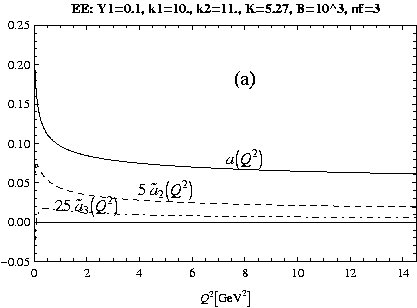
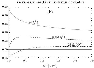
Figure 1: (a) Analytic coupling $a(Q^{2})$ (full line) at positive $0\leq Q^{2}<(3m_{c})^{2}$, in model EE; included are also higher order analytic couplings ${\widetilde{a}}_{2}(Q^{2})$ (dashed line) and ${\widetilde{a}}_{3}(Q^{2})$ (dot-dashed line) [cf. Eqs. (29)], for better visibility scaled by factors $5$ and $5^{2}$, respectively; (b) same as in (a), but at very low $Q^{2}>0$.

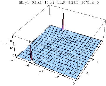
Figure 2: Absolute value of $\beta(F(z))$ in model EE as a function of $x$ and $y$ (where $z=x+iy$). The only pole is at $z_{\rm thr}=x_{\rm thr}\pm i\pi$. The physical sheet is $-\pi\leq y<\pi$.

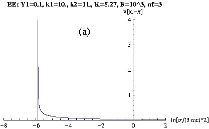
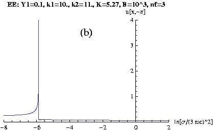
Figure 3: (a) Imaginary part ${\rm Im}F(z=x-i\pi)=v(x,-\pi)$ of the analytic coupling $F(z)=a(Q^{2})$ in model EE, as a function of $x$. Here, $v(x,-\pi)={\rm Im}a(Q^{2}=-\sigma-i\epsilon)=\rho_{1}(\sigma)$ is the usual discontinuity function of the analytic coupling, where $\sigma=\mu_{\rm in}^{2}\exp(x)$ ($\mu_{\rm in}=3m_{c}$, $m_{c}=1.27$ GeV). (b) Same for the real part ${\rm Re}F(z=x-i\pi)=u(x,-\pi)$.

All these results show that model EE is very similar to model P11, but significantly different from model P30. Further, the threshold values $x_{\rm thr}$ in models EE and P11 are similar (see Table 1): $x_{\rm thr}\approx-6.$; this corresponds to the threshold mass $Q^{2}_{\rm thr}=-M^{2}_{\rm thr}$ for the discontinuity function $\rho_{1}(\sigma)$ with values $M_{\rm thr}=(3m_{c})\exp(x_{\rm thr}/2)\approx 0.2$ GeV. On the other hand, in model P30, $x_{\rm thr}$ is much more negative: $x_{\rm thr}\approx-12.$, corresponding to $M_{\rm thr}\approx 0.01$ GeV. For all these reasons, we will consider models $EE$ and $P11$ as two viable models of analytic QCD which fulfill the conditions imposed at the outset of this letter.

In Figs. 1(a), (b) we present $a(Q^{2})$ and the higher order couplings ${\widetilde{a}}_{j}(Q^{2})$ ($j=2,3$) [cf. Eq. (29)], in model EE, as functions of $Q^{2}$ at low positive $Q^{2}\leq\mu^{2}_{\rm in}$. The Figure indicates strong hierarchy $a(Q^{2})\gg{\widetilde{a}}_{2}(Q^{2})\gg{\widetilde{a}}_{3}(Q^{2})\gg\ldots$ at all positive values of $Q^{2}$. In Fig. 2 we present the three-dimensional image of $|\beta(F(x+iy))|$ as a function of $x$ and $y$; we can see that there are no singularities of this function inside the $z$ stripe $-\pi<y(={\rm Im}(z))<+\pi$; the only singularity is at the threshold value $z_{\rm thr}=-5.8754-i\pi$ which corresponds to $Q^{2}\approx-(0.202)^{2}\ {\rm GeV}^{2}$ on the negative $Q^{2}$-axis. In Figs. 3 (a), (b) we present the behavior of the imaginary and real part of the coupling $F$ on the edge $z=x-i\pi$ [i.e., on the negative $Q^{2}$ axis: $Q^{2}=-\mu_{\rm in}^{2}\exp(x)$]. We see the threshold-type behavior at $z_{\rm thr}=x_{\rm thr}-i\pi=-5.8754-i\pi$. The fact that these latter curves have no (step-like) discontinuities at $x\not=x_{\rm thr}$ is an additional numerical indication that the function $F(z)$ has no singularities within the stripe $-\pi<{\rm Imz}<\pi$, i.e., no Landau singularities.

IV Summary

We investigated whether it is possible to construct analytic versions of QCD which obey the ITEP-OPE principle of no UV-contributions to power term corrections to pQCD $(\Lambda^{2}/Q^{2})^{n}$ and, at the same time, do not contradict the measured value of the semihadronic $\tau$ decay ratio $r_{\tau}$ (which is by far the most precisely measured low energy QCD quantity). We constructed such models by choosing specific forms for the RGE beta-function, and found that the answer is positive: such theories do exist. However, the obtained solutions came at a price, because the obtained series for $r_{\tau}$ show divergent behavior starting with the fifth term of the series. This was so because we had to introduce poles and zeros of the beta function on the imaginary axis relatively close to the origin (in the complex plane of the coupling), in order to increase the value of $r_{\tau}$. One model contained a cubic polynomial, another a simple Padé P[1/1] function, and yet another model a combination of exponential functions of the type $(\exp(-Y)-1)/Y$. The last two models show better apparent convergence behavior of $r_{\tau}$ (in the first four terms) and agree well with the (less precisely) measured values of the Bjorken polarized sum rule at low energies. The last two models appear to be numerically very similar to each other. We intend to use these two models in the future evaluations of various physical quantities with the OPE approach. This approach can be applied with the presented analytic QCD models since the latter respect the ITEP-OPE philosophy. For example, higher-twist contributions to the Bjorken polarized sume rule may be substantial. Such contributions were ignored in the numerical analysis here, but should eventually be included.

Appendix A Expansions and resummations of observables in analytic QCD

Here we refer to and summarize the approach decribed in our previous work CV2 . The massless stangeless ($\Delta S=0$) semihadronic $\tau$ decay ratio $r_{\tau}$ can be expressed in terms of the current-current correlation function $\Pi(Q^{2})$ (massless, V-V or A-A) as

$$r_{\tau}=\frac{2}{\pi}\int_{0}^{m^{2}_{\tau}}\ \frac{ds}{m^{2}_{\tau}}\left(1-\frac{s}{m^{2}_{\tau}}\right)^{2}\left(1+2\frac{s}{m^{2}_{\tau}}\right){\rm Im}\Pi(Q^{2}=-s)\ .$$ (25)

This integral can be transformed, via the use of Cauchy theorem in the $Q^{2}$-plane and the subsequent integration by parts, to the contour integral Braaten:1988hc ; Beneke:2008ad

$$r_{\tau}=\frac{1}{2\pi}\int_{-\pi}^{+\pi}d\phi\ (1+e^{i\phi})^{3}(1-e^{i\phi})\ d_{\rm Adl}(Q^{2}=m_{\tau}^{2}e^{i\phi})\ ,$$ (26)

where $d_{\rm Adl}(Q^{2})=-d\Pi(Q^{2})/d\ln Q^{2}$ is the (massless) Adler function whose perturbation expansion is

$$d_{\rm Adl.}(Q^{2}) = a+\sum_{n=1}^{\infty}d_{n}a^{n+1}$$ (27)

$$= a+\sum_{n=1}^{\infty}{\widetilde{d}}_{n}{\widetilde{a}}_{n+1}\ .$$ (28)

Here, the coupling parameter $a=a(\mu^{2};c_{2},c_{3},\ldots)$ is at a chosen RScl $\mu^{2}$ and in a chosen RSch $(c_{2},c_{3},\ldots)$ ($c_{n}\equiv\beta_{n}/\beta_{0}$), as are the coeffficients $d_{n}$ and ${\widetilde{d}}_{n}$: $d_{n}=d_{n}({\cal C};c_{2},\ldots,c_{n-1})$, ${\widetilde{d}}_{n}={\widetilde{d}}_{n}({\cal C};c_{2},\ldots,c_{n-1})$. Here, ${\cal C}$ is the dimensionless RScl parameter: ${\cal C}=\ln(\mu^{2}/Q^{2})$.

The higher order couplings ${\widetilde{a}}_{n+1}$ appearing in (28) are

$${\widetilde{a}}_{n+1}(\mu^{2})\equiv\frac{(-1)^{n}}{\beta_{0}^{n}n!}\frac{\partial^{n}a(\mu^{2})}{\partial(\ln\mu^{2})^{n}}\ ,\qquad(n=1,2,3,\ldots)\ .$$ (29)

The two expansions in (27) and (28) are in principle equivalent (not equivalent in practice, when truncation used), because of the relations

$${\widetilde{a}}_{2} = a^{2}+c_{1}a^{3}+c_{2}a^{4}+{\cal O}(a^{5})\,$$ (30)

$${\widetilde{a}}_{3} = a^{3}+(5/2)c_{1}a^{4}+{\cal O}(a^{5})\ ,\quad{\widetilde{a}}_{4}=a^{4}+{\cal O}(a^{5})\ ,\quad{\rm etc.}$$ (31)

and the consequent relations between $d_{n}$ and ${\widetilde{d}}_{m}$’s

$${\widetilde{d}}_{1} = d_{1}\ ,\quad{\widetilde{d}}_{2}=d_{2}-c_{1}d_{1}\ ,$$ (32)

$${\widetilde{d}}_{3} = d_{3}-(5/2)c_{1}d_{2}+\left[(5/2)c_{1}^{2}-c_{2}\right]d_{1}\ ,\quad{\rm etc.}$$ (33)

The leading-$\beta_{0}$ contribution (LB, in Refs. CV1 ; CV2 named leading-skeleton LS) to the massless nonstrange ratio $r_{\tau}$ was given in Ref. CV2 in Appendix C, Eqs. (C8)-(C11), using results of Refs. Neubert ; Neubert2 . It is the contour integration (26) of the LB-part $d_{\rm Adl}^{\rm(LB)}$ of Adler function expansion (28). While the LB part was written in Refs. CV1 ; CV2 in terms of the Minkowskian coupling $\mathfrak{A}_{1}$

$$r_{\tau}^{\rm(LB)}=\int_{0}^{\infty}\frac{dt}{t}\>F_{r}^{\cal{M}}(t)\>\mathfrak{A}_{1}(te^{\cal{\overline{C}}}m_{\tau}^{2})\ ,$$ (34)

where ${\cal{\overline{C}}}=-5/3$, the characteristic function $F_{r}^{\cal{M}}(t)$ is given in Eqs. (C10)-(C11) there, and the Minkowskian (time-like) coupling $\mathfrak{A}_{1}(\sigma)$ is related with the discontinuity (cut) function $\rho_{1}(\sigma)$ of the coupling parameter $a$ [$\rho_{1}(\sigma)\equiv{\rm Im}a(Q^{2}=-\sigma-i\epsilon)$] in the following way:

$$\frac{d}{d\ln\sigma}{\mathfrak{A}}_{1}(\sigma)=-\frac{1}{\pi}{\rho}_{1}(\sigma)\ .$$ (35)

Since the discontinuity function is $\rho_{1}(\sigma)={\rm Im}F(z)$ for $z=\ln(\sigma/\mu^{2}_{\rm in})-i\pi$, it is obtained as a direct byproduct of the integration of RGE (3). Thefore, it is convenient to express LB contribution (34) in terms of $\rho_{1}(\sigma)$ instead of ${\mathfrak{A}}_{1}(\sigma)$. This can be obtained from relation (34) by integration by parts and using relation (35)

$$r_{\tau}^{\rm(LB)}=\frac{1}{\pi}\int_{0}^{\infty}\frac{dt}{t}\>{\widetilde{F}}_{r}(t)\>\rho_{1}(te^{\cal{\overline{C}}}m_{\tau}^{2})\ ,$$ (36)

where

$${\widetilde{F}}_{r}(t)=\int_{0}^{t}\frac{dt^{\prime}}{t^{\prime}}\>F_{r}^{\cal{M}}(t^{\prime})\ .$$ (37)

Since $F_{r}^{\cal{M}}(t^{\prime})$ consists of powers of $t^{\prime}$ and polylogarithmic functions of $t^{\prime}$ and $1/t^{\prime}$, it turns out that integration in (37) can be performed analytically. Explicit expression for ${\widetilde{F}}_{r}(t)$ will be given in Ref. CKV . Here we only mention that ${\widetilde{F}}_{r}(t)\to 1$ when $t\to+\infty$, and that integration in (36) starts at a positive $t_{\rm thr}=(M^{2}_{\rm thr}/m_{\tau}^{2})\exp(-{\cal{\overline{C}}})$, due to the threshold behavior of $\rho_{1}(\sigma)$ in our presented models.

A systematic expansion of $r_{\tau}$ beyond the LB can then be written as $r_{\tau}^{\rm(LB)}$ plus contour integrals of ${\widetilde{a}}_{n+1}$’s ($n\geq 1$)

$$r_{\tau}=r_{\tau}^{\rm(LB)}+\sum_{n=1}^{\infty}\ T_{n}I({\widetilde{a}}_{n+1},{\cal C})\ ,$$ (38)

where

$$I({\widetilde{a}}_{n+1},{\cal C})=\frac{1}{2\pi}\int_{-\pi}^{+\pi}d\phi\ (1+e^{i\phi})^{3}(1-e^{i\phi})\ {\widetilde{a}}_{n+1}(e^{\cal C}m_{\tau}^{2}e^{i\phi})\ ,$$ (39)

${\cal C}$ is an (arbitrary) renormalization scale (RScl) parameter ($|{\cal C}|\stackrel{{\scriptstyle<}}{{\sim}}1$), and the coefficients $T_{j}$ are

$$T_{1} = {\overline{T}}_{1}={\overline{c}}_{10}^{(1)}=\frac{1}{12}\ ,$$ (40)

$$T_{2} = {\overline{T}}_{2}+2\beta_{0}{\cal C}\ {\overline{c}}_{10}^{(1)}-(c_{2}-{\overline{c}}_{2})\ ,$$ (41)

$$T_{3} = {\overline{T}}_{3}+3\beta_{0}\ {\cal C}{\overline{c}}_{10}^{(1)}(\beta_{0}{\overline{c}}_{11}^{(2)}+{\overline{c}}_{10}^{(2)})+3\ {\cal C}{\overline{c}}_{10}^{(1)}(\beta_{0}^{2}{\cal C}-\beta_{1})$$ (42)

$$+(c_{2}-{\overline{c}}_{2})\left((5/2)c_{1}-3{\overline{c}}_{10}^{(1)}-3\beta_{0}({\overline{c}}_{11}^{(1)}+{\cal C})\right)-(1/2)(c_{3}-{\overline{c}}_{3})\ .$$

The overlines indicate the corresponding quantities which appear in the ${\overline{\rm MS}}$ RSch with RScl parameter ${\cal C}=0$; coefficients $c_{ij}^{(k)}$ are determined by the $\beta_{0}$-expansions of the perturbation coefficients of the massless Adler function $d(Q^{2})$; for details see Ref. CV2 , particularly Appendix A. In particular, for $n_{f}=3$: $c_{10}^{(1)}=1/12$, $c_{11}^{(1)}=0.691772$; $c_{10}^{(2)}=-278.673$, $c_{11}^{(2)}=59.2824$. The ${\rm N}^{3}{\rm LB}$ coefficients ${\overline{T}}_{3}$ and $T_{3}$ can now be calculated exactly because the ${\rm N}^{3}{\rm LO}$ perturbative coefficient ${\overline{d}}_{3}$ of the massless Adler function is now known exactly d3 . In our case ($n_{f}=3$) it turns out that ${\overline{T}}_{2}=-12.2554$ and ${\overline{T}}_{3}=1.55291$.

Eq. (41) indicates that ${\rm N}^{3}{\rm LB}$ coefficient $T_{2}$ becomes large positive [and thus the ${\rm N}^{3}{\rm LB}$ term in expansion (38) becomes significant positive] if the beta-coefficient $c_{2}$ becomes negative: $c_{2}\ll-1$. Futhermore, if $|c_{4}|$ is large and dominant (as it is in our models), Eqs. (40)-(42) indicate that $T_{4}\approx-(1/3)c_{4}$ and thus $|T_{4}|$ is large.

If no LB-resummation is performed in $r_{\tau}$ ($\Leftrightarrow$ in $d_{\rm Adl.}$), then $r_{\tau}$ is obtained by performing contour integration (26) term-by-term for the sum (28)

$$r_{\tau}=I(a,{\cal C})+\sum_{n=1}^{\infty}\ {\widetilde{d}}_{n}I({\widetilde{a}}_{n+1},{\cal C})\ .$$ (43)

In practice, we have to truncate sums (38) and (43), by including $n_{\rm max}=3$ because only the first three coefficients $d_{n}$ ($\Leftrightarrow{\widetilde{d}}_{n}$) are known exactly d1 ; d2 ; d3 .

Bjorken polarized sum rule (BjPSR) $d_{\rm Bj}(Q^{2})$ is yet another QCD observable with measured values (although much less precisely than $r_{\tau}$) at low energies. It can be calculated in a similar way. Its perturbation expansion can be organized in two ways, like in Eqs. (27) and (28) for the Adler function. LB-resummation

$$d_{\rm Bj}(Q^{2})^{\rm(LB)}=\int_{0}^{\infty}\frac{dt}{t}\ F_{\rm Bj}(t)a(te^{\cal{\overline{C}}}Q^{2})\ ,$$ (44)

can be performed with the characteristic function obtained in Refs. CV1 ; CV2

$$F_{\rm Bj}(\tau)=\left\{\begin{array}[]{ll}\frac{8}{9}\tau\left(1-\frac{5}{8}\tau\right)&\tau\leq 1\\ \frac{4}{9\tau}\left(1-\frac{1}{4\tau}\right)&\tau\geq 1\end{array}\right\}\ .$$ (47)

Inclusion of terms beyond the LB gives

$$d_{\rm Bj}(Q^{2})=d_{\rm Bj}(Q^{2})^{\rm(LB)}+\sum_{n=1}^{\infty}(T_{\rm Bj})_{n}{\widetilde{a}}_{n+1}(e^{\cal C}Q^{2})\ ,$$ (48)

where coefficients $(T_{\rm Bj})_{n}$ are analogous to coefficients $T_{n}$ of Eqs. (40)-(42), but this time based on the BjPSR perturbation coefficients $({\widetilde{d}}_{\rm Bj})_{k}$ ($k=1,\ldots,n$) instead of ${\widetilde{d}}_{k}$ of Adler function. The perturbation coefficients $(d_{\rm Bj})_{1}$ and $(d_{\rm Bj})_{2}$ are known exactly LV , and for $(d_{\rm Bj})_{3}$ we use an estimate given in Ref. KS for $n_{f}=3$: $({\overline{d}}_{\rm Bj})_{3}\approx 130.$

If LB resummation is not performed, the resulting expression is

$$d_{\rm Bj}(Q^{2})=a(e^{\cal C}Q^{2})+\sum_{n=1}^{\infty}({\widetilde{d}}_{\rm Bj})_{n}{\widetilde{a}}_{n+1}(e^{\cal C}Q^{2})\ ,$$ (49)

where the perturbation coefficients $({\widetilde{d}}_{\rm Bj})_{n}$ are evaluated at the chosen RScl $\mu^{2}=\exp({\cal C})Q^{2}$ and in the RSch $(c_{2},c_{3},\ldots)$ dictated by $\beta$-functions of our analytic QCD models.

References

- (1) D. V. Shirkov and I. L. Solovtsov, hep-ph/9604363; Phys. Rev. Lett. 79, 1209 (1997) [hep-ph/9704333].
- (2) A. V. Nesterenko, Phys. Rev. D 62, 094028 (2000); Phys. Rev. D 64, 116009 (2001); Int. J. Mod. Phys. A 18, 5475 (2003); A. V. Nesterenko and J. Papavassiliou, Phys. Rev. D 71, 016009 (2005); A. C. Aguilar, A. V. Nesterenko and J. Papavassiliou, J. Phys. G 31, 997 (2005). J. Phys. G 32, 1025 (2006) [arXiv:hep-ph/0511215].
- (3) A. I. Alekseev, Few Body Syst. 40, 57 (2006) [arXiv:hep-ph/0503242].
- (4) Y. Srivastava, S. Pacetti, G. Pancheri and A. Widom, In the Proceedings of Physics at Intermediate Energies, SLAC, Stanford, CA, USA, 30 April - 2 May 2001, pp T19 [arXiv:hep-ph/0106005].
- (5) B. R. Webber, JHEP 9810, 012 (1998) [arXiv:hep-ph/9805484].
- (6) G. Cvetič and C. Valenzuela, J. Phys. G 32, L27 (2006) [arXiv:hep-ph/0601050];
- (7) G. Cvetič and C. Valenzuela, Phys. Rev. D 74, 114030 (2006) [arXiv:hep-ph/0608256].
- (8) G. M. Prosperi, M. Raciti and C. Simolo, Prog. Part. Nucl. Phys. 58, 387 (2007) [arXiv:hep-ph/0607209].
- (9) D. V. Shirkov and I. L. Solovtsov, Theor. Math. Phys. 150, 132 (2007) [arXiv:hep-ph/0611229].
- (10) G. Cvetič and C. Valenzuela, Braz. J. Phys. 38, 371 (2008) [arXiv:0804.0872 [hep-ph]].
- (11) G. Cvetič and C. Valenzuela, Phys. Rev. D 77, 074021 (2008) [arXiv:0710.4530 [hep-ph]].
- (12) M. A. Shifman, A. I. Vainshtein and V. I. Zakharov, Nucl. Phys. B 147, 385 (1979); Nucl. Phys. B 147, 448 (1979).
- (13) Y. L. Dokshitzer, G. Marchesini and B. R. Webber, Nucl. Phys. B 469, 93 (1996) [hep-ph/9512336].
- (14) K. A. Milton, I. L. Solovtsov and O. P. Solovtsova, Phys. Lett. B 415, 104 (1997); [hep-ph/9706409]; K. A. Milton, I. L. Solovtsov, O. P. Solovtsova and V. I. Yasnov, Eur. Phys. J. C 14, 495 (2000) [hep-ph/0003030].
- (15) B. V. Geshkenbein, B. L. Ioffe and K. N. Zyablyuk, Phys. Rev. D 64, 093009 (2001) [arXiv:hep-ph/0104048].
- (16) K. A. Milton, I. L. Solovtsov and O. P. Solovtsova, Phys. Rev. D 64, 016005 (2001) [arXiv:hep-ph/0102254].
- (17) T. A. Ryttov and F. Sannino, Phys. Rev. D 78 (2008) 065001 [arXiv:0711.3745 [hep-th]].
- (18) V. A. Novikov, M. A. Shifman, A. I. Vainshtein and V. I. Zakharov, Nucl. Phys. B 229 (1983) 381.
- (19) P. A. Ra̧czka, Nucl. Phys. Proc. Suppl. 164, 211 (2007) [arXiv:hep-ph/0512339]; hep-ph/0602085; hep-ph/0608196.
- (20) K. G. Chetyrkin, B. A. Kniehl and M. Steinhauser, Phys. Rev. Lett. 79, 2184 (1997) [arXiv:hep-ph/9706430].
- (21) W. Wetzel, Nucl. Phys. B 196, 259 (1982); W. Bernreuther and W. Wetzel, Nucl. Phys. B 197, 228 (1982) [Erratum-ibid. B 513, 758 (1998)]; W. Bernreuther, Annals Phys. 151, 127 (1983); Z. Phys. C 20, 331 (1983).
- (22) G. Rodrigo and A. Santamaria, Phys. Lett. B 313, 441 (1993) [arXiv:hep-ph/9305305].
- (23) S. A. Larin, T. van Ritbergen and J. A. M. Vermaseren, Nucl. Phys. B 438, 278 (1995) [arXiv:hep-ph/9411260].
- (24) Mathematica 7, Wolfram Co.
- (25) G. Cvetič, R. Kögerler and C. Valenzuela, in preparation.
- (26) E. Gardi, G. Grunberg and M. Karliner, JHEP 9807, 007 (1998) [arXiv:hep-ph/9806462].
- (27) A. Deur et al., Phys. Rev. Lett. 93, 212001 (2004) [hep-ex/0407007].
- (28) S. Schael et al. [ALEPH Collaboration], Phys. Rept. 421, 191 (2005) [arXiv:hep-ex/0506072].
- (29) M. Davier, A. Höcker and Z. Zhang, Rev. Mod. Phys. 78, 1043 (2006) [arXiv:hep-ph/0507078].
- (30) M. Davier, S. Descotes-Genon, A. Hocker, B. Malaescu and Z. Zhang, Eur. Phys. J. C 56, 305 (2008) [arXiv:0803.0979 [hep-ph]].
- (31) C. Amsler et al. [Particle Data Group], Phys. Lett. B 667, 1 (2008).
- (32) E. Braaten, Phys. Rev. Lett. 60, 1606 (1988); S. Narison and A. Pich, Phys. Lett. B 211, 183 (1988); E. Braaten, S. Narison, and A. Pich, Nucl. Phys. B 373, 581 (1992); A. Pich and J. Prades, JHEP9806, 013 (1998) [hep-ph/9804462].
- (33) M. Beneke and M. Jamin, JHEP 0809, 044 (2008) [arXiv:0806.3156 [hep-ph]].
- (34) M. Neubert, Phys. Rev. D 51, 5924 (1995) [hep-ph/9412265].
- (35) M. Neubert, arXiv:hep-ph/9502264.
- (36) P. A. Baikov, K. G. Chetyrkin and J. H. Kühn, Phys. Rev. Lett. 101, 012002 (2008) [arXiv:0801.1821 [hep-ph]].
- (37) K. G. Chetyrkin, A. L. Kataev and F. V. Tkachov, Phys. Lett. B 85, 277 (1979); M. Dine and J. R. Sapirstein, Phys. Rev. Lett. 43, 668 (1979); W. Celmaster and R. J. Gonsalves, Phys. Rev. Lett. 44, 560 (1980).
- (38) S. G. Gorishnii, A. L. Kataev and S. A. Larin, Phys. Lett. B 259, 144 (1991); L. R. Surguladze and M. A. Samuel, Phys. Rev. Lett. 66, 560 (1991) [Erratum-ibid. 66, 2416 (1991)].
- (39) S. G. Gorishny and S. A. Larin, Phys. Lett. B 172, 109 (1986); E. B. Zijlstra and W. Van Neerven, Phys. Lett. B 297, 377 (1992); S. A. Larin and J. A. M. Vermaseren, Phys. Lett. B 259, 345 (1991).
- (40) A. L. Kataev and V. V. Starshenko, Mod. Phys. Lett. A 10, 235 (1995) [hep-ph/9502348].