Synchrosqueezed Wavelet Transforms: a Tool for Empirical Mode Decomposition

Abstract

The EMD algorithm, first proposed in [11], made more robust as well as more versatile in [13], is a technique that aims to decompose into their building blocks functions that are the superposition of a (reasonably) small number of components, well separated in the time-frequency plane, each of which can be viewed as approximately harmonic locally, with slowly varying amplitudes and frequencies. The EMD has already shown its usefulness in a wide range of applications including meteorology, structural stability analysis, medical studies – see, e.g. [12]. On the other hand, the EMD algorithm contains heuristic and ad-hoc elements that make it hard to analyze mathematically.

In this paper we describe a method that captures the flavor and philosophy of the EMD approach, albeit using a different approach in constructing the components. We introduce a precise mathematical definition for a class of functions that can be viewed as a superposition of a reasonably small number of approximately harmonic components, and we prove that our method does indeed succeed in decomposing arbitrary functions in this class. We provide several examples, for simulated as well as real data.

1 Introduction

Time-frequency representations provide a powerful tool for the analysis of time dependent signals. They can give insight into the complex structure of a “multi-layered” signal consisting of several components, such as the different phonemes in a speech utterance, or a sonar signal and its delayed echo. There exist many types of time-frequency (TF) analysis algorithms; the overwhelming majority belong to either “linear” or “quadratic” methods.

In “linear” methods, the signal to be analyzed is characterized by its inner products with (or correlations with) a pre-assigned family of templates, generated from one (or a few) basic template by simple operations. Examples are the windowed Fourier transform, where the family of templates is generated by translating and modulating a basic window function, or the wavelet transform, where the templates are obtained by translating and dilating the basic (or “mother”) wavelet. Many linear methods, including the windowed Fourier transform and the wavelet transform, make it possible to reconstruct the signal from the inner products with templates; this reconstruction can be for the whole signal, or for parts of the signal; in the latter case, one typically restricts the reconstruction procedure to a subset of the TF plane. However, in all these methods, the family of template functions used in the method unavoidably “colors” the representation, and can influence the interpretation given on “reading” the TF representation in order to deduce properties of the signal. Moreover, the Heisenberg uncertainty principle limits the resolution that can be attained in the TF plane; different trade-offs can be achieved by the choice of the linear transform or the generator(s) for the family of templates, but none is ideal, as illustrated in Figure 1.

 

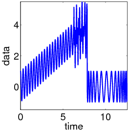
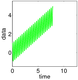
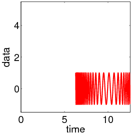
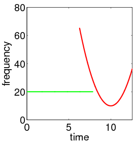
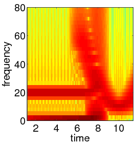
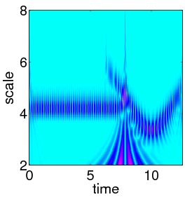
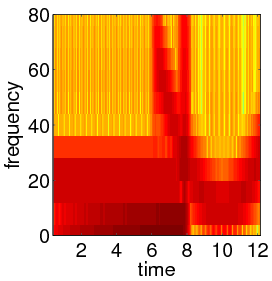
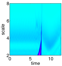
Figure 1: Examples of linear time-frequency representations.                                                      Top row: the signal $s(t)=s_{1}(t)+s_{2}(t)$ (top left) defined by $s_{1}(t)=.5t+\cos(20t)$ for $0\leq t\leq 5\pi/2$, (top middle) and $s_{2}(t)=\cos\left(\frac{4}{3}\,[(t-10)^{3}-(2\pi-10)^{3}]+10(t-2\pi)\right)$ for $2\pi\leq t\leq 4\pi$ (top right); Next row: Left:the instantaneous frequency for its two components(left) $\omega(t)=20$ for $0\leq(t-10)^{2}\leq 5\pi/2$, and $\omega(t)=4t^{2}+10$ for $2\pi\leq t\leq 4\pi$; Middle: two examples of (the absolute value of) a continuous windowed Fourier transform of $s(t)$, with a wide window (top) and a narrow window (bottom) [these are plotted with Matlab, with the ‘jet’ colormap]; Right: two examples of a continuous wavelet transform of $s(t)$, with a Morlet wavelet (top) and a Haar wavelet (bottom) [plotted with ‘hsv’ colormap in Matlab]. The instantaneous frequency profile can be clearly recognized in each of these linear TF representations, but it is “blurred” in each case, in different ways that depend on the choice of the transform.

In “quadratic” methods to build a TF representation, one can avoid introducing a family of templates with which the signal is “compared” or “measured”. As a result, some features can have a crisper, “more focused” representation in the TF plane with quadratic methods (see Figure 2).

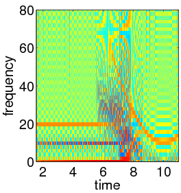
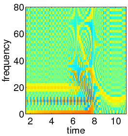
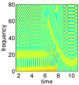
Figure 2: Examples of quadratic time-frequency representations. Left: the Wigner-Ville transform of $s(t)$, in which interference causes the typical Moiré patterns; Middle and Right: two pseudo-Wigner-Ville transforms of $s(t)$, obtained by blurring the Wigner-Ville transform slightly (middle) and somehwat more (right). [All three graphs plotted with ‘jet’ colormap in Matlab, calibrated identically.] The blurring removes the interference patterns, at the cost of precise location in the time-frequency localization.

However, in this case, “reading” the TF representation of a multi-component signal is rendered more complicated by the presence of interference terms between the TF representations of the individual components; these interference effects also cause the “time-frequency density” to be negative in some parts of the TF plane. These negative parts can be removed by some further processing of the representation [8], at the cost of reintroducing some blur in the TF plane again. Reconstruction of the signal, or part of the signal, is much less straightforward for quadratic than for linear TF representations.

In many practical applications, in a wide range of fields (including, e.g., medicine and engineering) one is faced with signals that have several components, all reasonably well localized in TF space, at different locations. The components are often also called “non-stationary”, in the sense that they can present jumps or changes in behavior, which it may be important to capture as accurately as possible. For such signals both the linear and quadratic methods come up short. Quadratic methods obscure the TF representation with interference terms; even if these could be dealt with, reconstruction of the individual components would still be an additional problem. Linear methods are too rigid, or provide too blurred a picture. Figures 1, 2 show the artifacts that can arise in linear or quadratic TF representations when one of the components suddenly stops or starts. Figure 3 shows examples of components that are non harmonic, but otherwise perfectly reasonable as candidates for a single-component-signal, yet not well represented by standard TF methods, as illustrated by the lack of concentration in the time-frequency plane of the transforms of these signals.

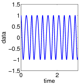
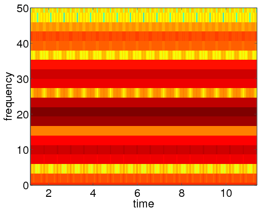
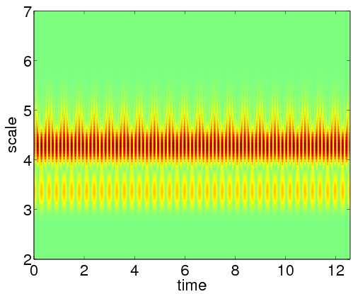
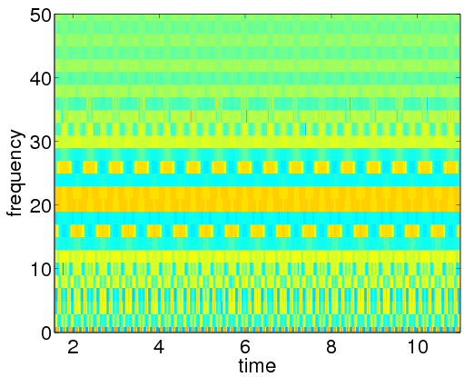
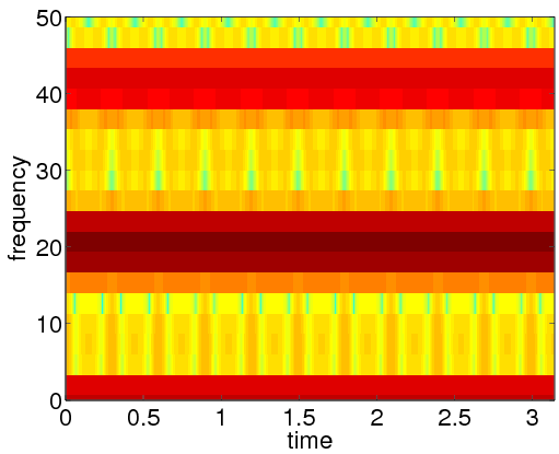
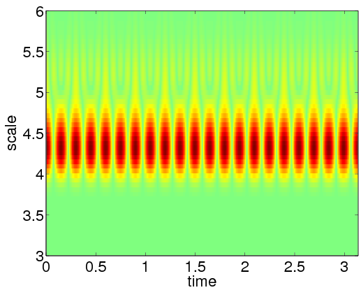
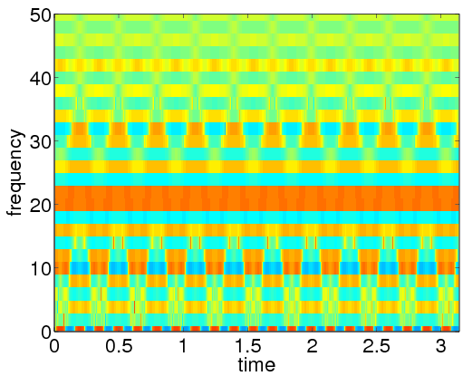
Figure 3: Two examples of wave functions of the type $\cos[\phi(t)]$, with slowly varying $A(t)$ and $\phi^{\prime}(t)$, for which standard TF representations are not very well localized in the time-frequence plane. Left: signal, Middle left: windowed Fourier transform; Middle Right: Morlet wavelet transform; Right: Wigner-Ville function. [All TF representations plotted with ‘jet’ colormap in Matlab.]

The Empirical Mode Decomposition (EMD) method was proposed by Norden Huang [11] as an algorithm that would allow time-frequency analysis of such multicomponent signals, without the weaknesses sketched above, overcoming in particular artificial spectrum spread caused by sudden changes. Given a signal $s(t)$, the method decomposes it into several instrinsic mode functions (IMF):

$$s(t)\,=\,\sum_{k=1}^{K}s_{k}(t),$$ (1.1)

where each IMF is basically a function oscillating around 0, albeit not necessarily with constant frequency:

$$s_{k}(t)\,=\,A_{k}(t)\,\cos(\phi_{k}(t))~{},~{}\mbox{ with }A_{k}(t),\,\phi^{\prime}_{k}(t)>0~{}\forall t~{}.$$ (1.2)

Essentially, each IMF is an amplitude modulated-frequency modulated (AM-FM) signal; typically, the change in time of $A_{k}(t),\,\phi^{\prime}_{k}(t)$ is much slower than the change of $\phi_{k}(t)$ itself, which means that locally (i.e. in a time interval $[t-\delta,t+\delta]$, with $\delta\approx 2\pi[\phi^{\prime}_{k}(t)]^{-1}$) the component $s_{k}(t)$ can be regarded as a harmonic signal with amplitude $A_{k}(t)$ and frequency $\phi_{k}^{\prime}(t)$. (In [11], the conditions on an IMF are phrased as follows: (1) in the whole data set, the number of extrema and the number of zero crossings of $s_{k}(t)$ must either be equal or differ at most by one; and (2) at any $t$, the value of a smooth envelope defined by the local minima of the IMF is the negative of the corresponding envelope defined by the local maxima.) After the decomposition of $s(t)$ into its IMF components, the EMD algorithm proceeds to the computation of the “instantaneous frequency” of each component. Theoretically, this is given by $\omega_{k}(t)\,:=\,\phi^{\prime}_{k}(t)$; in practice, rather than a (very unstable) differentiation of the estimated $\phi_{k}(t)$, the originally proposed EMD method used the Hilbert transform of the $s_{k}(t)$ [11]; more recently, this has been replaced by other methods [13].

It is obvious that every function can be written in the form (1.1) with each component as in (1.2). If $s(t)$ is supported (or observed) in $[-T,T]$, then the Fourier series on $[-T,T]$ of $s(t)$ is actually such a decomposition. It is also easy to see that such a decomposition is far from unique. This is simply illustrated by considering the following signal:

$$s(t)\,=\,.25\,\cos([\Omega-\gamma]t)\,+\,2.5\,\cos(\Omega t)\,+\,.25\,\cos([\Omega+\gamma]t)\,=\,\left(\,2\,+\,\cos^{2}\left[\,\frac{\gamma}{2}\,t\,\right]\,\right)\,\cos(\,\Omega t)~{},$$ (1.3)

where $\Omega\gg\gamma$, so that one can set $A(t)\,:=\,2\,+\,\cos^{2}\left[\,\frac{\gamma}{2}\,t\,\right]\,,$ which varies much more slowly than $\cos[\phi(t)]\,=\,\cos[\Omega\,t]$.

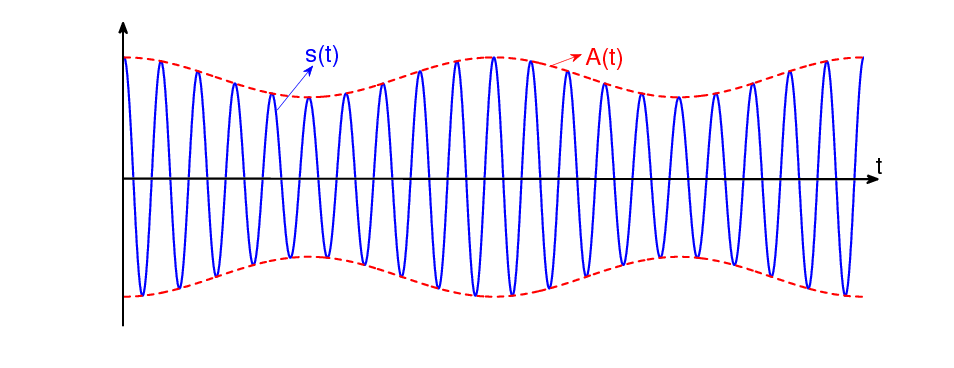
Figure 4: Ṉon-uniqueness for decomposition into IMT. This function can be considered as a single component, of the type $A(t)\cos[\Omega t]$, with slowly varying amplitude, or as the sum of three components. (See text.)

The interpretation of this signal is not unique: It can be regarded either as a summation of three cosines with frequencies $\Omega-\gamma$, $\Omega$ and $\Omega+\gamma$ respectively, or as a single component with frequency $\Omega$ which has an amplitude $A(t)$ that is slowly modulated. Depending on the circumstances, either interpretation can be the “best”. In the EMD’s framework, the second interpretation (single component, with slowly varying amplitude) is preferred when $\Omega\gg\gamma$; the EMD is typically applied when it is more “physically meaningful” to decompose a signal into fewer components if this can be achieved by mild variations in frequency and amplitude; in those circumstances, this preference is sensible. The (toy) example illustrates that we should not expect a universal solution to all TF decomposition problems. For certain classes of functions, consisting of a (reasonably) small number of components, well separated in the TF plane, each of which can be viewed as approximately harmonic locally, with slowly varying amplitdes and frequencies, it is clear, however, that a technique that identifies these components accurately, even in the presence of noise, has great potential for a wide range of applications. Such a decomposition should be able to accommodate such mild variations within the building blocks of the decomposition.

The EMD algorithm, first proposed in [11], made more robust as well as more versatile in [13] (an extension to higher dimensions is now possible), is such a technique. It has already shown its usefulness in a wide range of applications including meteorology, structural stability analysis, medical studies – see, e.g. [5, 6, 11]; a recent review is given in [12]. On the other hand, the EMD algorithm contains a number of heuristic and ad-hoc elements that make it hard to analyze mathematically its guarantees of accuracy or the limitations of its applicability. For instance, the EMD algorithm, uses a sifting process to construct the decomposition of type (1.1). In each step in this sifting process, two smooth interpolating functions are constructed (using cubic splines), one of the local maxima ($\bar{s}(t)$), and one of the local minima ($\underline{s}(t)$). From these interpolates, a mean curve of the signal is defined as $m(t)=(\bar{s}(t)+\underline{s}(t))/2$, which is then subtracted from the signal: $r_{1}(t)=s(t)-m(t)$. In most cases, $r_{1}$ is not yet a satisfactory IMF; the process is then repeated on $r_{1}$ again, etc $\ldots$; this repeated process is called “sifting”. Sifting is done for either a fixed number of times, or until a certain stopping criterium is satisfied; the final remainder $r_{n}(t)$ is taken as the first IMF, $s_{1}:=r_{n}$. The algorithm continues with the difference between the original signal and the first IMF to extract the second IMF (which is the first IMF obtained from the “new starting signal” $s(t)-s_{1}(t)$) and so on. (Examples of the decomposition will be given in Section 5.) Because the sifting process relies heavly on interpolates of maxima and minima, the end result has some stability problems in the presence of noise, as illustrated in [18]. The solution proposed in [18] addresses these issues in practice, but poses new challenges to our mathematical understanding.

Attempts at a mathematical understanding of the approach and the results produced by the EMD method have been mostly exploratory. A systematic investigation of the performance of EMD acting on white noise was carried out in [9, 17]; it suggests that in some limit, EMD on signals that don’t have structure (like white noise) produces a result akin to wavelet analysis. The decomposition of signals that are superpositions of a few cosines was studied in [16], with interesting results. A first different type of study, more aimed at building a mathematical framework, is given in [14, 10], which analyzes mathematically the limit of an infinite number of “sifting” operations, showing it defines a bounded operator on $\ell_{\infty}$, and studies its mathematical properties.

In summary, the EMD algorithm has shown its usefulness in various applications, yet our mathematical understanding of it is still very sketchy. In this paper we discuss a method that captures the flavor and philosophy of the EMD approach, without necessarily using the same approach in constructing the components. We hope this approach will provide new light in understanding of what makes EMD work, when it can be expected to work (and when not) and what type of precision we can expect.

2 Synchrosqueezing Wavelet Transforms

Synchrosqueezing was introduced in the context of analyzing auditory signals [7]; it is a special case of reallocation methods [1, 3, 4], which aim to “sharpen” a time-frequency representation $\mathcal{R}(t,\omega)$ by “allocating” its value to a different point $(t^{\prime},\omega^{\prime})$ in the time-frequency plane, determined by the local behavior of $\mathcal{R}(t,\omega)$ around $(t,\omega)$. In the case of synchrosqueezing, one reallocates the coefficients resulting from a continuous wavelet transform to get a concentrated time-frequency picture, from which instantaneous frequency lines can be extracted.

To motivate the idea, let us start with a purely harmonic signal,

$$s(t)=A\cos(\omega t).$$

Take a wavelet $\psi$ that is concentrated on the positive frequency axis: $\hat{\psi}(\xi)=0$ for $\xi<0$. Denote by $W_{s}(a,b)$ the continuous wavelet transform of $s$ defined by this choice of $\psi$. We have

$$\begin{split}W_{s}(a,b)&=\int s(t)\,a^{-1/2}\,\overline{\psi\bigl{(}\frac{t-b}{a}\bigr{)}}\,\mathrm{d}t\\ &=\frac{1}{2\pi}\int\hat{s}(\xi)\,a^{1/2}\,\overline{\hat{\psi}(a\xi)}\,e^{ib\xi}\,\mathrm{d}\xi\\ &=\frac{A}{4\pi}\int[\delta(\xi-\omega)+\delta(\xi+\omega)]\,a^{1/2}\,\overline{\hat{\psi}(a\xi)}\,e^{ib\xi}\,\mathrm{d}\xi\\ &=\frac{A}{4\pi}\,a^{1/2}\,\overline{\hat{\psi}(a\omega)}\,e^{ib\omega}.\end{split}$$ (2.1)

If $\hat{\psi}(\xi)$ is concentrated around $\xi=\omega_{0}$, then $W_{s}(a,b)$ will be concentrated around $a=\omega_{0}/\omega$. However, the wavelet transform $W_{s}(a,b)$ will be spread out over a region around the horizontal line $a=\omega_{0}/\omega$ on the time-scale plane. The observation made in [7] is that although $W_{s}(a,b)$ is spread out in $a$, its oscillatory behavior in $b$ points to the original frequency $\omega$, regardless of the value of $a$.

This led to the suggestion to compute, for any $(a,b)$ for which $W_{s}(a,b)\neq 0$, a candidate instantaneous frequency $\omega(a,b)$ by

$$\omega(a,b)=-i(W_{s}(a,b))^{-1}\frac{\partial}{\partial b}W_{s}(a,b).$$ (2.2)

For the purely harmonic signal $s(t)=A\cos(\omega t)$, one obtains $\omega(a,b)=\omega$, as desired; this is illustrated in Figure 5

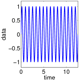
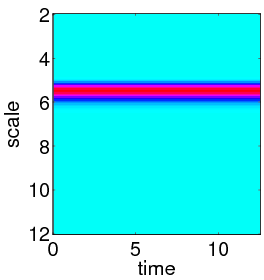
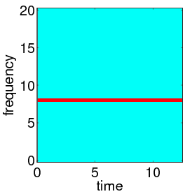
Figure 5: Left: the harmonic signal $f(t)=\sin(8t)$; Middle: the continuous wavelet transform of $f$; Right: synchrosqueezed transform of $f$.

In a next step, the information from the time-scale plane is transferred to the time-frequency plane, according to the map $(b,a)\longrightarrow(b,\omega(a,b))$, in an operation dubbed synchrosqueezing. In [7], the frequency variable $\omega$ and the scale variable $a$ were “binned”, i.e. $W_{s}(a,b)$ was computed only at discrete values $a_{k}$, with $a_{k}-a_{k-1}=(\Delta a)_{k}$, and its synchrosqueezed transform $T_{s}(\omega,b)$ was likewise determined only at the centers $\omega_{\ell}$ of the successive bins $\left[\omega_{\ell}-\frac{1}{2}\Delta\omega,\omega_{\ell}+\frac{1}{2}\Delta\omega\right]$, with $\omega_{\ell}-\omega_{\ell-1}=\Delta\omega$, by summing different contributions:

$$T_{s}(\omega_{\ell},b)=(\Delta\omega)^{-1}\sum_{a_{k}:\lvert\omega(a_{k},b)-\omega_{l}\rvert\leq\Delta\omega/2}W_{s}(a_{k},b)\,a_{k}^{-3/2}\,(\Delta a)_{k}.$$ (2.3)

The following argument shows that the signal can still be reconstructed after the synchrosqueezing. We have

$$\begin{split}\int_{0}^{\infty}W_{s}(a,b)\,a^{-3/2}\,\mathrm{d}a&=\frac{1}{2\pi}\int_{-\infty}^{\infty}\int_{0}^{\infty}\hat{s}(\xi)\,\overline{\hat{\psi}(a\xi)}\,e^{ib\xi}\,a^{-1}\,\mathrm{d}a\,\mathrm{d}\xi\\ &=\frac{1}{2\pi}\int_{0}^{\infty}\int_{0}^{\infty}\hat{s}(\xi)\,\overline{\hat{\psi}(a\xi)}\,e^{ib\xi}\,a^{-1}\,\mathrm{d}a\,\mathrm{d}\xi\\ &=\int_{0}^{\infty}\overline{\hat{\psi}(\xi)}\,\frac{\,\mathrm{d}\xi}{\xi}\cdot\frac{1}{2\pi}\int_{0}^{\infty}\hat{s}(\zeta)\,e^{ib\zeta}\,\mathrm{d}\zeta.\end{split}$$ (2.4)

Setting $C_{\psi}\,=\,2\int_{0}^{\infty}\overline{\hat{\psi}(\xi)}\,\frac{\,\mathrm{d}\xi}{\xi}$, we then obtain (assuming that $s$ is real, so that $\hat{s}(\xi)=\overline{\hat{s}(-\xi)}$, hence $s(b)=(4\pi)^{-1}\mathfrak{Re}\left[\int_{0}^{\infty}\hat{s}(\xi)\,e^{ib\xi}\,\mathrm{d}\xi\,\right]\,$)

$$s(b)=\mathfrak{Re}\left[C_{\psi}^{-1}\,\int_{0}^{\infty}W_{s}(a,b)\,a^{-3/2}\,\mathrm{d}a\,\right].$$ (2.5)

In the piecewise constant approximation corresponding to the binning in $a$, this becomes

$$s(b)\approx\mathfrak{Re}\left[C_{\psi}^{-1}\,\sum_{k}W_{s}(a_{k},b)\,a_{k}^{-3/2}\,(\Delta a)_{k}\,\right]\,=\,\mathfrak{Re}\left[C_{\psi}^{-1}\,\sum_{\ell}T_{s}(\omega_{\ell},b)\,(\Delta\omega)\right].$$ (2.6)

Remark.

As defined above, (2.3) implicitly assumes a linear scale discretization of $\omega$. If instead logarithmic discretization is used, the $\Delta\omega$ has to be made dependent on $\ell$; alternatively, one can also change the exponent of $a$ from $-3/2$ to $-1/2$.

If one chooses (as we shall do here) to continue to treat $a$ and $\omega$ as continuous variables, without discretization, the analog of (2.3) is

$$\mathcal{T}_{s}(\omega,b)=\int_{A(b)}W_{s}(a,b)\,a^{-3/2}\,\delta(\,\omega(a,b)-\omega\,)\,\mathrm{d}a,$$ (2.7)

where $A(b)=\{\,a\,;\,W_{s}(a,b)\neq 0\,\}$, and $\omega(a,b)$ is as defined in (2.2) above, for $(a,b)$ such that $a\in\,A(b)$.

Remark.

In practice, the determination of those $(a,b)$-pairs for which $W_{s}(a,b)=0$ is rather unstable, when $s$ has been contaminated by noise. For this reason, it is often useful to consider a threshold for $\lvert W_{s}(a,b)\rvert$, below which $\omega(a,b)$ is not defined; this amounts to replacing $A(b)$ by the smaller region $A_{\epsilon}(b):=\{a\,;\,\lvert W_{s}(a,b)\rvert\geq\epsilon\,\}$.

One can also view synchrosqueezing as follows. For sufficiently “nice” $s$ and $\psi$, we have, for $a\in A(b)$,

$$\omega(a,b) =-i(W_{s}(a,b))^{-1}\frac{\partial}{\partial b}W_{s}(a,b)$$ (2.8)

$$=\frac{\int\xi\,\hat{s}(\xi)\,\overline{\hat{\psi}(a\xi)}\,e^{ib\xi}\,\mathrm{d}\xi}{\int\hat{s}(\xi)\,\overline{\hat{\psi}(a\xi)}\,e^{ib\xi}\,\mathrm{d}\xi}$$ (2.9)

$$=\frac{\int-is^{\prime}(t)\,a^{-1/2}\,\overline{\psi\bigl{(}\frac{t-b}{a}\bigr{)}}\,\mathrm{d}t}{\int s(t)\,a^{-1/2}\,\overline{\psi\bigl{(}\frac{t-b}{a}\bigr{)}}\,\mathrm{d}t}$$ (2.10)

$$=\frac{\int-i\,(s+iHs)^{\prime}(t)\,a^{-1/2}\,\overline{\psi\bigl{(}\frac{t-b}{a}\bigr{)}}\,\mathrm{d}t}{\int(s+iHs)(t)\,a^{-1/2}\,\overline{\psi\bigl{(}\frac{t-b}{a}\bigr{)}}\,\mathrm{d}t},$$ (2.11)

where $Hs$ denotes the Hilbert transform of $s$; the last equality uses that $\hat{\psi}$ is supported on the positive frequencies only. If now $s$ is a so-called “asymptotic signal”, i.e., if

$$s(t)=a(t)\cos(\phi(t)),$$ (2.12)

with $a^{\prime}(t)\ll 1$ and $\phi^{\prime\prime}(t)\ll\phi^{\prime}(t)$, then the Hilbert transform of $s$ is (approximately) given by

$$Hs(t)\sim a(t)\sin(\phi(t)).$$ (2.13)

Therefore, using the above expression of $\omega(a,b)$, we have approximately

$$\omega(a,b) \sim\frac{\int a(t)\,\phi^{\prime}(t)\,e^{i\phi(t)}\,a^{-1/2}\,\overline{\psi\bigl{(}\frac{t-b}{a}\bigr{)}}\,\mathrm{d}t}{\int a(t)\,e^{i\phi(t)}\,a^{-1/2}\,\overline{\psi\bigl{(}\frac{t-b}{a}\bigr{)}}\,\mathrm{d}t}\sim\phi^{\prime}(b),$$ (2.14)

where, in the first approximation, we have omitted the term containing $a^{\prime}(t)$ as $a^{\prime}(t)\ll\phi^{\prime}(t)$, and in the second approximation, we have used that $\psi$ is localized around $0$.

This heuristic argument suggests that, for asymptotic signals, synchrosqueezing an appropriate wavelet transform will indeed give a single line on the time-frequency plane, at the value of the “instantaneous frequency” of a (putative) IMF.

3 Main Result

We define a class of functions, containing intrinsic mode type components that are well-separated, and show that they can be identified and characterized by means of synchrosqueezing.

We start with the following definitions:

Definition 3.1.

[Intrinsic Mode Type Function]
A function $f:\mathbb{R}\rightarrow\mathbb{C}$ is said to be intrinsic-mode-type (IMT) with accuracy $\epsilon\,>\,0$ if $f$ and $A\,:=\,|f|$ have the following properties:

$$f(t)\,= \,A(t)\,e^{i\phi(t)}~{}~{}~{}~{}~{}\mbox{ where } A\in C^{1}(\mathbb{R}),\,\phi\in C^{2}(\mathbb{R})$$

$$\inf_{t\in\mathbb{R}}\phi^{\prime}(t)\,>\,0~{}~{},$$

$$|A^{\prime}(t)|,\,|\phi^{\prime\prime}(t)|\leq\epsilon\,|\phi^{\prime}(t)|\,,\,\forall t\in\mathbb{R}$$

$$M^{\prime\prime}\,:=\,\sup_{t\in\mathbb{R}}|\phi^{\prime\prime}(t)|<\infty~{}.$$

Definition 3.2.

[Superposition of Well-Separated Intrinsic Mode Components]
A function $f:\mathbb{R}\rightarrow\mathbb{C}$ is said to be a superposition of, or to consist of, well-separated Intrinsic Mode Components, up to accuracy $\epsilon$, and with separation $d$ if it can be written as

$$f(t)\,=\,\sum_{k=1}^{K}\,f_{k}(t)\,$$

where all the $f_{k}$ are IMT, and where moreover their respective phase functions $\phi_{k}$ satisfy

$$\phi^{\prime}_{k}(t)>\phi^{\prime}_{k-1}(t)\,,~{}~{}\mbox{ and }~{}~{}~{}|\phi^{\prime}_{k}(t)\,-\,\phi^{\prime}_{k-1}(t)|\geq d[\phi^{\prime}_{k}(t)\,+\,\phi^{\prime}_{k-1}(t)]\,,\quad\forall t\in\mathbb{R}\,.$$

Remark.

It is not really necessary for the components $f_{k}$ to be defined on all of $\mathbb{R}$. One can also suppose that they are supported on intervals, $\operatorname{supp}(f_{k})\,=\,\operatorname{supp}(A_{k})\subset[-T_{k},T_{k}]$, where the different $T_{k}$ need not be identical. In this case the various inequalities governing the definition of an IMT function or a superposition of well-separated IMT components must simply be restricted to the relevant intervals. For the inequality above on the $\phi^{\prime}_{k}(t),\,\phi^{\prime}_{k-1}(t)$, it may happen that some $t$ are covered by (say) $[-T_{k},T_{k}]$ but not by $[-T_{k-1},T_{k-1}]$; one should then replace $k-1$ by the largest $\ell<k$ for which $t\in[-T_{\ell},T_{\ell}]$; other, similar, changes would have to be made if $t\in[-T_{k-1},T_{k-1}]\setminus[-T_{k},T_{k}]$.
We omit this extra wrinkle for the sake of keeping notations manageable.

Notation.

[Class $\mathcal{A}_{\epsilon,d}$]
We denote by $\mathcal{A}_{\epsilon,d}$ the set of all superpositions of well-separated IMT, up to accuracy $\epsilon$ and with separation $d$.

Our main result is then the following:

Theorem 3.3.

[Main result]
Let $f$ be a function in $\mathcal{A}_{\epsilon,d}$, and set $\widetilde{\epsilon}:=\epsilon^{1/3}$. Pick a wavelet $\psi$ such that its Fourier transform $\widehat{\psi}$ is supported in $[1-\Delta,1+\Delta]$, with $\Delta<d/(1+d)$, and set $\mathcal{R}_{\psi}\,=\,\sqrt{2\pi}\,\int\,\widehat{\psi}(\zeta)\,\zeta^{-1}\,d\zeta\,$. Consider the continuous wavelet transform $W_{f}(a,b)$ of $f$ with respect to this wavelet, as well as the function $S_{f,\sigma}(b,\omega)$ obtained by synchrosqueezing $W_{f}$, with threshold $\widetilde{\epsilon}$, i.e.

$$S_{f,\widetilde{\epsilon}}(b,\omega)\,:=\,\int_{A_{\widetilde{\epsilon},f}(b)}\,W_{f}(a,b)\,\delta(\omega-\omega_{f}(a,b))\,a^{-3/2}\,da~{},$$

where $A_{\widetilde{\epsilon},f}(b)\,:=\,\{a\in\mathbb{R}_{+}\,;\,|W_{f}(a,b)|\,>\,\widetilde{\epsilon}\,\}~{}.$
Then, provided $\epsilon$ (and thus also $\widetilde{\epsilon}$) is sufficiently small, the following hold:
 
$\bullet\,|W_{f}(a,b)|\,>\,\widetilde{\epsilon}$ only when, for some $k\in\{1,\ldots,K\}~{}$, $(a,b)\in Z_{k}\,:=\,$ $\{(a,b)\,;\,|\,a\,\!\phi^{\prime}_{k}(b)\,-\,1\,|\,<\,\Delta\}\,$.
 
$\bullet$ For each $k\in\{1,\ldots,K\}$, and for each pair $(a,b)\in Z_{k}$ for which $|W_{f}(a,b)|\,>\,\widetilde{\epsilon}$, we have

$$|\omega_{f}(a,b)\,-\,\phi^{\prime}_{k}(b)\,|\,\leq\,\widetilde{\epsilon}~{}.$$

$\bullet$ Moreover, for each $k\in\{1,\ldots,K\}$, there exists a constant $C$ such that, for any $b\in\mathbb{R}$,

$$\left|\,\left(\,\mathcal{R}_{\psi}^{-1}\int_{|\omega-\phi^{\prime}_{k}(b)|<\widetilde{\epsilon}}\,S_{f,\widetilde{\epsilon}}(b,\omega)\,d\omega\,\right)\,-\,A_{k}(b)\,e^{i\,\phi_{k}(b)}\,\right|\,\leq\,C\,\widetilde{\epsilon}~{}.$$

This theorem basically tells us that, for $f\in\mathcal{A}_{\epsilon,d}$, the synchrosqueezed version $S_{f,\widetilde{\epsilon}}$ of the wavelet transform $W_{f}$ is completely concentrated, in the $(t,\omega)$-plane, in narrow bands around the curves $\omega\,=\,\phi^{\prime}_{k}(t)$, and that the restriction of $S_{f,\widetilde{\epsilon}}$ to the $k$-th narrow band suffices to reconstruct, with high precision, the $k$-th IMT component of $f$. Synchrosqueezing (an appropriate) wavelet transform thus provides the adaptive time-frequency decomposition that is the goal of Empirical Mode Decomposition.

The proof of Theorem 3.3 relies on a number of estimates, which we demonstrate one by one, at the same time providing more details about what it means for $\epsilon$ to be “sufficiently small”. In the statement and proof of all the estimates in this section, we shall always assume that all the conditions of Theorem 3.3 are satisfied (without repeating them), unless stated otherwise.

The first estimate bounds the growth of the $A_{k}$, $\phi^{\prime}_{k}$ in the neighborhood of $t$, in terms of the value of $|\phi^{\prime}_{k}(t)|$.

Estimate 3.4.

For each $k\in\{1,\ldots,K\}$, we have

$$|A_{k}(t+s)\,-\,A_{k}(t)|\,\leq\,\epsilon\,|s|\,\left(\,|\phi^{\prime}_{k}(t)|\,+\,\frac{1}{2}\,M^{\prime\prime}_{k}\,|s|\,\right)~{}~{}\mbox{ and }~{}~{}|\phi^{\prime}_{k}(t+s)\,-\,\phi^{\prime}_{k}(t)|\,\leq\,\epsilon\,|s|\,\left(\,|\phi^{\prime}_{k}(t)|\,+\,\frac{1}{2}\,M^{\prime\prime}_{k}\,|s|\,\right)~{}.$$

Proof.

$$\left|\,A_{k}(t+s)\,-\,A_{k}(t)\,\right|\, = \,\left|\,\int_{0}^{s}\,A^{\prime}_{k}(t+u)\,du\,\right|$$

$$\leq \,\int_{0}^{s}\,\left|\,A^{\prime}_{k}(t+u)\right|\,du\,\leq\,\epsilon\,\int_{0}^{s}\,\left|\,\phi^{\prime}_{k}(t+u)\right|\,du~{}.$$

$$= \,\epsilon\,\int_{0}^{s}\,\left|\,\phi^{\prime}_{k}(t)\,+\,\int_{0}^{u}\,\phi^{\prime\prime}_{k}(t+u)\,du\,\right|\,dt\,\leq\,\epsilon\,\left(\,\left|\phi^{\prime}_{k}(t)\right|\,|s|\,+\,\frac{1}{2}\,M^{\prime\prime}_{k}\,|s|^{2}\,\right)~{}.$$

The other bound is analogous. ∎

The next estimate shows that, for $f$and $\psi$ as given in the statement of Theorem 3.3, the wavelet transform $W_{f}(a,b)$ is concentrated near the regions where, for some $k\in\{1,2,\ldots,K\}$, $~{}a\,\!\phi^{\prime}_{k}(b)~{}$ is close to 1.

Estimate 3.5.

$$\left|\,W_{f}(a,b)\,-\,\sqrt{2\pi}\,\sum_{k=1}^{K}\,A_{k}(b)\,e^{i\phi_{k}(b)}\,\sqrt{a}\,\widehat{\psi}\left(a\,\phi^{\prime}_{k}(b)\right)\,\right|\,\leq\,\epsilon\,a^{3/2}\,\Gamma_{1}~{},$$

where

$$\Gamma_{1}\,:=\,I_{1}\sum_{k=1}^{K}\,|\phi_{k}^{\prime}(b)|\,+\,\frac{1}{2}\,I_{2}\,a\,\sum_{k=1}^{K}\,\left[\,M^{\prime\prime}_{k}\,+\,|A_{k}(b)|\,|\phi_{k}^{\prime}(b)|\,\right]\,+\,\frac{1}{6}\,I_{3}\,a^{2}\,\sum_{k=1}^{K}\,M^{\prime\prime}_{k}\,|A_{k}(b)|~{},$$

with $I_{n}\,:=\,\int\,|u|^{n}\,|\psi(u)|\,du~{}$.

Proof.

We have

$$W_{f}(a,b)\, = \,\sum_{k=1}^{K}\,\int\,A_{k}(t)\,e^{i\phi_{k}(t)}\,a^{-1/2}\,\psi\left(\frac{t-b}{a}\right)\,dt$$

$$= \,\sum_{k=1}^{K}\,A_{k}(b)\,\int\,e^{i[\phi_{k}(b)\,+\,\phi_{k}^{\prime}(b)\,(t-b)\,+\,\int_{0}^{t-b}[\phi_{k}^{\prime}(b+u)-\phi_{k}^{\prime}(b)]du]}\,a^{-1/2}\,\psi\left(\frac{t-b}{a}\right)\,dt$$

$$~{}~{}~{}~{}~{}~{}~{}~{}~{}\,+\,\sum_{k=1}^{K}\,[A_{k}(t)\,-\,A_{k}(b)]\,e^{i\phi_{k}(t)}\,a^{-1/2}\,\psi\left(\frac{t-b}{a}\right)\,dt~{}.$$

It follows that

$$\left|\,W_{f}(a,b)\,-\,\sqrt{2\pi}\,\sum_{k=1}^{K}\,A_{k}(b)\,e^{i\phi_{k}(b)}\,\sqrt{a}\,\widehat{\psi}\left(a\,\phi^{\prime}_{k}(b)\right)\,\right|\,$$

$$\quad\leq\,\sum_{k=1}^{K}\,\int\,\left|A_{k}(t)\,-\,A_{k}(b)\right|\,a^{-1/2}\,\left|\psi\left(\frac{t-b}{a}\right)\right|\,dt$$

$$\quad\quad\quad\quad\,+\,\sum_{k=1}^{K}\,|A_{k}(b)|\,\int\,\left|e^{i\int_{0}^{t-b}[\phi^{\prime}_{k}(b+u)-\phi^{\prime}_{k}(b)]du}\,-\,1\right|\,a^{-1/2}\,\left|\psi\left(\frac{t-b}{a}\right)\right|\,dt$$

$$\quad\leq\,\sum_{k=1}^{K}\,\int\,\epsilon\,|t-b|\left(|\phi^{\prime}_{k}(b)|+\frac{1}{2}\,M_{k}^{\prime\prime}\,|t-b|\right)\,a^{-1/2}\,\left|\psi\left(\frac{t-b}{a}\right)\right|\,dt$$

$$\quad\quad\quad\quad\,+\,\sum_{k=1}^{K}\,|A_{k}(b)|\,\int\,\left|\int_{0}^{t-b}[\phi^{\prime}_{k}(b+u)-\phi^{\prime}_{k}(b)]du\right|\,a^{-1/2}\,\left|\psi\left(\frac{t-b}{a}\right)\right|\,dt$$

$$\quad\leq\,\epsilon\sum_{k=1}^{K}\,\left[\,a^{3/2}\,|\phi_{k}^{\prime}(b)|\,\int\,|u|\,|\psi(u)|\,du\,+\,a^{5/2}\,\frac{1}{2}\,M^{\prime\prime}_{k}\,\int\,|u|^{2}\,|\psi(u)|\,du\,\right]$$

$$\quad\quad\quad\quad\,+\,\sum_{k=1}^{K}\,|A_{k}(b)|\,\epsilon\,\int\,\left[\,\frac{1}{2}\,|t-b|^{2}\,|\phi^{\prime}_{k}(b)|\,+\,\frac{1}{6}\,|t-b|^{3}\,M^{\prime\prime}_{k}\right]\,a^{-1/2}\,\left|\psi\left(\frac{t-b}{a}\right)\right|\,dt$$

$$\quad\leq\epsilon\,a^{3/2}\,\left\{I_{1}\sum_{k=1}^{K}\,|\phi_{k}^{\prime}(b)|\,+\,\frac{1}{2}\,I_{2}\,a\,\sum_{k=1}^{K}\,\left[\,M^{\prime\prime}_{k}\,+\,|A_{k}(b)|\,|\phi_{k}^{\prime}(b)|\,\right]\,+\,\frac{1}{6}\,I_{3}\,a^{2}\,\sum_{k=1}^{K}\,M^{\prime\prime}_{k}\,|A_{k}(b)|\,\right\}$$

∎

The wavelet $\psi$ satisfies $\widehat{\psi}(\xi)\neq 0$ only for $1-\Delta<\xi<1+\Delta$; it follows that $|W_{f}(a,b)|\,\leq\,\epsilon\,a^{3/2}\,\Gamma_{1}$ whenever $|\,a\,\phi^{\prime}_{k}(b)\,-\,1\,|\,>\,\Delta$ for all $k\in\{1,\ldots,K\}$. On the other hand, we also have the following lemma:

Lemma 3.6.

For any pair $(a,b)$ under consideration, there can be at most one $k\in\{1,\ldots,K\}$ for which $|\,a\,\phi^{\prime}_{k}(b)\,-\,1\,|\,<\,\Delta$.

Proof.

Suppose that $k,\,\ell\in\{1,\ldots,K\}$ both satisfy the condition, i.e. that $|\,a\,\phi^{\prime}_{k}(b)\,-\,1\,|\,<\,\Delta$ and $|\,a\,\phi^{\prime}_{\ell}(b)\,-\,1\,|\,<\,\Delta$, with $k\neq\ell$. For the sake of definiteness, assume $k>\ell$. Since $f\in\mathcal{A}_{\epsilon,d}$, we have

$$\phi^{\prime}_{k}(b)-\phi^{\prime}_{\ell}(b)\,\geq\,\phi^{\prime}_{k}(b)-\phi^{\prime}_{k-1}(b)\,\geq\,\ d\,[\phi^{\prime}_{k}(b)+\phi^{\prime}_{k-1}(b)]\,\geq\,\ d\,[\phi^{\prime}_{k}(b)+\phi^{\prime}_{\ell}(b)]~{}.$$

Combined with

$$\phi^{\prime}_{k}(b)-\phi^{\prime}_{\ell}(b) \leq\,a^{-1}\,[\,(1+\Delta)\,-\,(1-\Delta)\,]\,=\,2\,a^{-1}\,\Delta~{},$$

$$\phi^{\prime}_{k}(b)+\phi^{\prime}_{\ell}(b) \geq\,a^{-1}\,[\,(1-\Delta)\,-\,(1-\Delta)\,]\,=\,2\,a^{-1}\,(1-\Delta)~{},$$

this gives

$$\,\Delta\,\geq\,d\,(1-\Delta)~{},$$

which contradicts the condition $\Delta\,<\,d/(1+d)$ from Theorem 3.3. ∎

It follows that the $a,b$-plane contains $K$ non-touching “zones”, corresponding to $|\,a\,\phi^{\prime}_{k}(b)\,-\,1\,|\,<\,\Delta$, $k\in\{1,\ldots,K\}$, separated by a “no-man’s land” where $|W_{f}(a,b)|$ is small. We shall assume (see below) that $\epsilon$ is sufficiently small, i.e., that for all $(a,b)$ under consideration,

$$\epsilon\,<\,a^{-9/4}\,\Gamma_{1}^{-3/2}~{},$$ (3.1)

so that $\epsilon\,a^{3/2}\,\Gamma_{1}\,<\,\epsilon^{1/3}\,=\,\widetilde{\epsilon}$. The upper bound in the intermediate region between the $K$ special zones is then below the threshold allowed $\widetilde{\epsilon}$ for the computation of $\omega_{f}(a,b)$ used in $S_{f,\widetilde{\epsilon}}$ (see the formulation of Theorem 3.3). It follows that we will compute $\omega_{f}(a,b)$ only in the special zones themselves. We thus need to estimate $\partial_{b}W_{f}(a,b)$ in each of these zones.

Estimate 3.7.

For $k\in\{1,\ldots,K\}$, and $(a,b)\in\mathbb{R}_{+}\times\mathbb{R}$ such that $|\,a\,\phi^{\prime}_{k}(b)\,-\,1\,|\,<\,\Delta$, we have

$$\left|\,-i\,\partial_{b}\,W_{f}(a,b)\,-\,\sqrt{2\pi}\,A_{k}(b)\,e^{i\phi_{k}(b)}\,\sqrt{a}\,\phi^{\prime}_{k}(b)\,\widehat{\psi}\left(a\,\phi^{\prime}_{k}(b)\right)\,\right|\,\leq\,\epsilon\,a^{1/2}\,\Gamma_{2}~{},$$

where

$$\Gamma_{2}\,:=\,I^{\prime}_{1}\sum_{k=1}^{K}\,|\phi_{k}^{\prime}(b)|\,+\,\frac{1}{2}\,I^{\prime}_{2}\,a\,\sum_{k=1}^{K}\,\left[\,M^{\prime\prime}_{k}\,+\,|A_{k}(b)|\,|\phi_{k}^{\prime}(b)|\,\right]\,+\,\frac{1}{6}\,I^{\prime}_{3}\,a^{2}\,\sum_{k=1}^{K}\,M^{\prime\prime}_{k}\,|A_{k}(b)|~{},$$

with $I^{\prime}_{n}\,:=\,\int\,|u|^{n}\,|\psi^{\prime}(u)|\,du~{}$.

Proof.

The proof follows the same lines as that for Estimate 3.5. We have

$$\partial_{b}\,W_{f}(a,b) =\,\partial_{b}\,\left(\,\sum_{\ell=1}^{K}\,\int\,A_{\ell}(t)\,e^{i\phi_{\ell}(t)}\,a^{-1/2}\,\psi\left(\frac{t-b}{a}\right)\,dt\,\right)$$

$$=\,-\,a^{-3/2}\,\sum_{\ell=1}^{K}\,\int\,A_{\ell}(t)\,e^{i\phi_{\ell}(t)}\,\,\psi^{\prime}\left(\frac{t-b}{a}\right)\,dt\,$$

$$=\,-\,\sum_{\ell=1}^{K}\,A_{\ell}(b)\,\int\,e^{i[\phi_{\ell}(b)\,+\,\phi_{\ell}^{\prime}(b)\,(t-b)\,+\,\int_{0}^{t-b}[\phi_{\ell}^{\prime}(b+u)-\phi_{\ell}^{\prime}(b)]du]}\,a^{-3/2}\,\psi^{\prime}\left(\frac{t-b}{a}\right)\,dt$$

$$\quad\quad\quad\,-\,\sum_{\ell=1}^{K}\,[A_{\ell}(t)\,-\,A_{\ell}(b)]\,e^{i\phi_{\ell}(t)}\,a^{-3/2}\,\psi^{\prime}\left(\frac{t-b}{a}\right)\,dt~{}.$$

By Lemma 3.6, only the term for $\ell=k$ survives in the sum for $(a,b)$ such that $|\,a\,\phi^{\prime}_{k}(b)\,-\,1\,|\,<\,\Delta$, and we obtain

$$\,\left|\partial_{b}\,W_{f}(a,b)\,-\,i\,\sqrt{2\pi}\,A_{k}(b)\,e^{i\phi_{k}(b)}\,\sqrt{a}\,\phi^{\prime}_{k}(b)\widehat{\psi}\left(a\,\phi^{\prime}_{k}(b)\right)\,\right|$$

$$\quad\,=\,\left|\partial_{b}\,W_{f}(a,b)\,-\,\sqrt{2\pi}\,A_{k}(b)\,e^{i\phi_{k}(b)}\,\frac{1}{\sqrt{a}}\,\widehat{\psi^{\prime}}\left(a\,\phi^{\prime}_{k}(b)\right)\,\right|\,$$

$$\quad\leq\,\int\,\epsilon\,|t-b|\left(|\phi^{\prime}_{k}(b)|+\frac{1}{2}\,M^{\prime\prime}\,|t-b|\right)\,a^{-3/2}\,\left|\psi^{\prime}\left(\frac{t-b}{a}\right)\right|\,dt$$

$$\quad\quad\quad\quad\,+\,|A_{k}(b)|\,\int\,\left|e^{i\int_{0}^{t-b}[\phi^{\prime}_{k}(b+u)-\phi^{\prime}_{k}(b)]du}\,-\,1\right|\,a^{-3/2}\,\left|\psi^{\prime}\left(\frac{t-b}{a}\right)\right|\,dt$$

$$\quad\leq\,\epsilon\,\left[\,a^{1/2}\,|\phi_{k}^{\prime}(b)|\,\int\,|u|\,|\psi^{\prime}(u)|\,du\,+\,a^{3/2}\,\frac{1}{2}\,M^{\prime\prime}_{k}\,\int\,|u|^{2}\,|\psi^{\prime}(u)|\,du\,\right]$$

$$\quad\quad\quad\quad\,+\,|A_{k}(b)|\,\epsilon\,\int\,\left[\,\frac{1}{2}\,|t-b|^{2}\,|\phi^{\prime}_{k}(b)|\,+\,\frac{1}{6}\,|t-b|^{3}\,M^{\prime\prime}_{k}\right]\,a^{-3/2}\,\left|\psi^{\prime}\left(\frac{t-b}{a}\right)\right|\,dt$$

$$\quad\leq\epsilon\,a^{1/2}\,\left\{I^{\prime}_{1}\,|\phi_{k}^{\prime}(b)|\,+\,\frac{1}{2}\,I^{\prime}_{2}\,a\,\left[\,M^{\prime\prime}_{k}\,+\,|A_{k}(b)|\,|\phi_{k}^{\prime}(b)|\,\right]\,+\,\frac{1}{6}\,I^{\prime}_{3}\,a^{2}\,M^{\prime\prime}_{k}\,|A_{k}(b)|\,\right\}$$

∎

Combining Estimates 3.5 and 3.7, we find

Estimate 3.8.

Suppose that (3.1) is satisfied. For $k\in\{1,\ldots,K\}$, and $(a,b)\in\mathbb{R}_{+}\times\mathbb{R}$ such that both $|\,a\,\phi^{\prime}_{k}(b)\,-\,1\,|\,<\,\Delta$ and $W_{f}(a,b)\geq\widetilde{\epsilon}$ are satisfied, we have

$$\left|\,\omega_{f}(a,b)\,-\,\phi^{\prime}_{k}(b)\,\right|\,\leq\,\sqrt{a}\,\left(\,\Gamma_{2}\,+\,a\,\Gamma_{1}\,\phi^{\prime}_{k}(b)\,\right)\,\epsilon^{2/3}~{}.$$

Proof.

By definition,

$$\omega_{f}(a,b)\,=\,\frac{-i\partial_{b}W_{f}(a,b)}{W_{f}(a,b)}~{}.$$

For convenience, let us, for this proof only, denote $\sqrt{2\pi}\,A_{k}(b)\,e^{i\phi_{k}(b)}\,\sqrt{a}\,\widehat{\psi}\left(a\,\phi^{\prime}_{k}(b)\right)$ by B. For the $(a,b)$-pairs under consideration, we have then

$$|\,-i\,\partial_{b}W_{f}(a,b)\,-\,\phi^{\prime}_{k}(b)\,B\,|\,\leq\,\epsilon\,a^{1/2}\,\Gamma_{2}\quad\mbox{and}\quad|W_{f}(a,b)-\,B\,|\,\leq\,\epsilon\,a^{3/2}\,\Gamma_{1}~{}.$$

Using $\widetilde{\epsilon}\,=\,\epsilon^{1/3}$, it follows that

$$\omega_{f}(a,b)\,-\,\phi^{\prime}_{k}(b)\,=\,\frac{-i\partial_{b}W_{f}(a,b)\,-\,\phi^{\prime}_{k}(b)\,B}{W_{f}(a,b)}\,+\,\frac{[B\,-\,W_{f}(a,b)]\,\phi^{\prime}_{k}(b)}{W_{f}(a,b)}~{},$$

so that

$$\left|\,\omega_{f}(a,b)\,-\,\phi^{\prime}_{k}(b)\,\right|\,\leq\,\frac{\epsilon\,a^{1/2}\,\Gamma_{2}\,+\,\epsilon\,a^{3/2}\,\phi^{\prime}_{k}(b)\,\Gamma_{1}}{W_{f}(a,b)}\,\leq\,\sqrt{a}\,\left(\,\Gamma_{2}\,+\,a\,\Gamma_{1}\,\phi^{\prime}_{k}(b)\,\right)\,\epsilon^{2/3}~{}.$$

∎

If (see below) we impose an extra restriction on $\epsilon$, namely that, for all $(a,b)$ under consideration, and all $k\in\{1,\ldots,K\}\,$,

$$\epsilon\,\leq\,a^{-3/2}\,\left[\,\Gamma_{2}\,+\,a\,\phi^{\prime}_{k}(b)\,\Gamma_{1}\,\right]^{-3}~{},$$ (3.2)

then this last estimate can be simplified to

$$\left|\,\omega_{f}(a,b)\,-\,\phi^{\prime}_{k}(b)\,\right|\,\leq\,\widetilde{\epsilon}~{}.$$ (3.3)

Next is our final estimate:

Estimate 3.9.

Suppose that both (3.1) and (3.2) are satisfied, and that, in addition, for all $b$ under consideration,

$$\epsilon\,\leq\,1/8\,d^{3}\,[\,\phi^{\prime}_{1}(b)\,+\,\phi^{\prime}_{2}(b)\,]^{3}~{}.$$ (3.4)

Let $S_{f,\widetilde{\epsilon}}$ be the synchrosqueezed wavelet transform of $f$,

$$S_{f,\widetilde{\epsilon}}(b,\omega)\,:=\,\int_{A_{\widetilde{\epsilon},f}(b)}\,W_{f}(a,b)\,\delta(\omega-\omega_{f}(a,b))\,a^{-3/2}\,da~{}.$$

Then we have, for all $b\in\mathbb{R}$, and all $k\in\{1,\ldots,K\}$

$$\left|\,\mathcal{R}_{\psi}^{-1}\int_{|\omega-\phi^{\prime}_{k}(b)|<\widetilde{\epsilon}}\,S_{f,\sigma}(b,\omega)\,d\omega\,-\,A_{k}(b)\,e^{i\phi_{k}(b)}\,\right|\,\leq\,C\widetilde{\epsilon}~{}.$$

Proof.

For later use, note first that (3.4) implies that, for all $k,\,\ell\in\{1,\ldots,K\}$,

$$d\,[\,\phi^{\prime}_{k}(b)\,+\,\phi^{\prime}_{\ell}(b)\,]\,>\,2\,\widetilde{\epsilon}~{}.$$ (3.5)

We have

$$\int_{|\omega-\phi^{\prime}_{k}(b)|<\widetilde{\epsilon}}\,S_{f,\sigma}(b,\omega)\,d\omega =\,\int_{|\omega-\phi^{\prime}_{k}(b)|<\widetilde{\epsilon}}\,\int_{A_{\widetilde{\epsilon},f}(b)}\,W_{f}(a,b)\,\delta(\omega\,-\,\omega_{f}(a,b))\,a^{-3/2}\,da\,d\omega$$

$$=\,\int_{A_{\widetilde{\epsilon},f}(b)\cap\{|\omega_{f}(a,b)-\phi_{k}^{\prime}(b)|<\widetilde{\epsilon}\}}\,W_{f}(a,b)\,a^{-3/2}\,da~{}.$$

From Estimate 3.5 and (3.1) we know that $|W_{f}(a,b)|>\widetilde{\epsilon}$ only when $|a\phi_{\ell}^{\prime}(b)-1|<\Delta$ for some $\ell\in\{1,\ldots,K\}$. For $\ell\neq k$, we have (use (3.5))

$$|\omega_{f}(a,b)-\phi^{\prime}_{\ell}(b)| \geq\,|\phi^{\prime}_{\ell}(b)-\phi^{\prime}_{k}(b)|\,-\,|\omega_{f}(a,b)-\phi^{\prime}_{k}(b)|$$

$$\geq\,d\,[\,\phi^{\prime}_{\ell}(b)+\phi^{\prime}_{k}(b)\,]\,-\,\widetilde{\epsilon}\,>\,\widetilde{\epsilon}~{},$$

which, by Estimate 3.8, implies that $|a\phi_{\ell}^{\prime}(b)-1|\geq\Delta$. Hence

$$\int_{|\omega-\phi^{\prime}_{k}(b)|<\widetilde{\epsilon}}\,S_{f,\sigma}(b,\omega)\,d\omega =\,\int_{A_{\widetilde{\epsilon},f}(b)\cap\{|a\phi_{k}^{\prime}(b)-1|<\Delta\}}\,W_{f}(a,t)\,a^{-3/2}\,da$$

$$=\,\left(\int_{|a\phi_{k}^{\prime}(b)-1|<\Delta}\,W_{f}(a,b)\,a^{-3/2}\,da\right)\,$$

$$\quad\quad\quad\quad-\,\left(\int_{\{|a\phi_{k}^{\prime}(b)-1|<\Delta\}\backslash A_{\widetilde{\epsilon},f}(b)}\,W_{f}(a,b)\,a^{-3/2}\,da\,\right)~{}.$$

From Estimate 3.5 we then obtain

$$\left|\,\mathcal{R}_{\psi}^{-1}\,\int_{|\omega-\phi^{\prime}_{k}(b)|<\widetilde{\epsilon}}\,S_{f,\sigma}(b,\omega)\,d\omega\,-\,\,A_{k}(b)\,e^{i\phi_{k}(b)}\,\right|\,$$

$$\quad\quad\leq\,\left|\,\mathcal{R}_{\psi}^{-1}\,\left(\int_{|a\phi_{k}^{\prime}(b)-1|<\Delta}\,W_{f}(a,b)\,a^{-3/2}\,da\right)\,-\,A_{k}(b)\,e^{i\phi_{k}(b)}\,\right|\,$$

$$\quad\quad\quad\quad\quad\quad+\,\mathcal{R}_{\psi}^{-1}\,\left|\int_{\{|a\phi_{k}^{\prime}(b)-1|<\Delta\}\backslash A_{\widetilde{\epsilon},f}(b)}\,W_{f}(a,b)\,a^{-3/2}\,da\right|$$

$$\quad\quad\leq\,\left|\,\mathcal{R}_{\psi}^{-1}\,\sqrt{2\pi}\,A_{k}(b)\,e^{i\phi_{k}(b)}\,\left(\int_{|a\phi^{\prime}_{k}(b)-1|<\Delta)}\,\sqrt{a}\,\widehat{\psi}(a\phi^{\prime}_{k}(b))\,a^{-3/2}\,da\,\right)\,-\,A_{k}(b)\,e^{i\phi_{k}(b)}\,\right|$$

$$\quad\quad\quad\quad\quad\quad+\,\mathcal{R}_{\psi}^{-1}\,\int_{|a\phi^{\prime}_{k}(b)-1|<\Delta)}\,\left[\,\widetilde{\epsilon}\,+\,\widetilde{\epsilon}\,a^{-3/2}\,\right]\,da~{}.$$

For the first term on the right hand side, since

$$\mathcal{R}_{\psi}^{-1}\,\sqrt{2\pi}\,A_{k}(b)\,e^{i\phi_{k}(b)}\,\int_{|a\phi^{\prime}_{k}(b)-1|<\Delta}\,\widehat{\psi}(a\phi^{\prime}_{k}(b))\,a^{-1}\,da\\ =\,\mathcal{R}_{\psi}^{-1}\,\sqrt{2\pi}\,A_{k}(b)\,e^{i\phi_{k}(b)}\,\int_{|\zeta-1|<\Delta}\,\widehat{\psi}(\zeta)\,\zeta^{-1}\,d\zeta\ \,=\,A_{k}(b)\,e^{i\phi_{k}(b)}~{},$$

by the definition of $\mathcal{R}_{\psi}$, and hence the first term vanishes. We thus obtain

$$\left|\,\mathcal{R}_{\psi}^{-1}\,\int_{|\omega-\phi^{\prime}_{k}(b)|<\widetilde{\epsilon}}\,S_{f,\sigma}(t,\omega)\,d\omega\,-\,\,A_{k}(b)\,e^{i\phi_{k}(b)}\,\right|\,\leq\,2\,\widetilde{\epsilon}\,\mathcal{R}_{\psi}^{-1}\,\left[\,\frac{\Delta}{\phi^{\prime}_{k}(b)}\,+\,\left(\frac{\phi^{\prime}_{k}(b)}{1-\Delta}\right)^{1/2}\,-\,\left(\frac{\phi^{\prime}_{k}(b)}{1+\Delta}\right)^{1/2}\right]$$

∎

It is now easy to see that all the Estimates together provide a complete proof for Theorem 3.3.

Remark.

We have three different conditions on $\epsilon$, namely (3.1), (3.2) and (3.4). The auxiliary quantities in these inequalities depend on $a$ and $b$, and the conditions should be satisfied for all $(a,b)$-pairs under consideration. This is not really a problem: the dependence on $b$ is via the quantities $A_{k}(b)$ and $\phi^{\prime}_{k}(b)$, and it is reasonable to assume these are uniformly bounded above and below (away from zero); because the bounds on the $\phi^{\prime}_{k}(b)$ translate into bounds on $a$, we can likewise safely assume that $a$ is bounded above as well as below (away from zero). Note that the different terms can be traded off in many other ways than what is done here; no effort has been made to optimize the bounds, and they can surely be improved. The focus here was not on optimizing the constants, but on proving that, if the rate of change (in time) of the $A_{k}(b)$ and the $\phi^{\prime}_{k}(b)$ is small, compared with the rate of change of the $\phi_{k}(b)$ themselves, then synchrosqueezing will identify both the “instantaneous frequencies” and their amplitudes.
In the statement of Theorem 3.3, we required the wavelet $\psi$ to have a compactly supported Fourier transform. This is not absolutely necessary; it was done here for convenience in the proof. If $\widehat{\psi}$ is not compactly supported, then extra terms occur in many of the estimates, taking into account the decay of $\widehat{\psi}(\zeta)$ as $\zeta\rightarrow\infty$ or $\zeta\rightarrow 0$; these can be handled in ways similar to what we saw above, at the cost of significantly lengthening the computations without making a conceptual difference.

4 A Variational Approach

The construction and estimates in the previous section can also be interpreted in a variational framework.

Let us go back to the notion of “instantaneous frequency.” Consider a signal $s(t)$ that is a sum of IMT components $s_{i}(t)$:

$$s(t)=\sum_{i=1}^{N}s_{i}(t)=\sum_{i=1}^{N}A_{i}(t)\,\cos(\phi_{i}(t)),$$ (4.1)

with the additional constraints that $\phi_{i}^{\prime}(t)$ and $\phi_{j}^{\prime}(t)$ for $i\not=j$ are “well separated”, so that it is reasonable to consider the $s_{i}$ as individual components. According to the philosophy of EMD, the instantaneous frequency at time $t$, for the $i$-th component, is then given by $\omega_{i}(t)=\phi_{i}^{\prime}(t)$.

How could we use this to build a time-frequency representation for $s$? If we restrict ourselves to a small window in time around $T$, of the type $[T-\Delta t,T+\Delta t]$, with $\Delta t\approx 2\pi/\phi_{i}^{\prime}(T)$, then (by its IMT nature) the $i$-th component can be written (approximately) as

$$\left.s_{i}(t)_{\!{}_{\,}}\right|_{[T-\Delta t,T+\Delta t]}\approx A_{i}(T)\,\cos\left[\phi_{i}(T)+\phi_{i}^{\prime}(T)\,(t-T)\right],$$

which is essentially a truncated Taylor expansion in which terms of size $O(A^{\prime}_{i}(T))$, $O(\phi^{\prime\prime}_{i}(T))$ have been neglected. Introducing $\omega_{i}(T)=\phi_{i}^{\prime}(T)$, and the phase $\varphi_{i}(T):=\phi_{i}(T)-\omega_{i}(T)T$ we can rewrite this as

$$\left.s_{i}(t)_{\!{}_{\,}}\right|_{[T-\Delta t,T+\Delta t]}\approx A_{i}(T)\,\cos\left[\omega_{i}(T)t+\varphi_{i}(T)\right].$$

This signal has a time-frequency representation, as a bivariate “function” of time and frequency, given by (for $t\in[T-\Delta t,T+\Delta t]$)

$$F_{i}(t,\omega)=A_{i}(T)\,\cos[\omega t+\varphi_{i}(T)]\,\delta(\omega-\omega_{i}(T)),$$ (4.2)

where $\delta$ is the Dirac-delta measure. The time-frequency representation for the full signal $s=\sum_{i=1}^{N}s_{i}$, still in the neighborhood of $t=T$, would then be

$$F(t,\omega)=\sum_{i=1}^{N}A_{i}(T)\,\cos[\omega t+\varphi_{i}(T)]\,\delta(\omega-\omega_{i}(T)).$$ (4.3)

Integrating over $\omega$, in the neighborhood of $t=T$, leads to $s(t)\approx\int F(t,\omega)\,\mathrm{d}\omega$.

All this becomes even simpler if we introduce the “complex form” of the time-frequency representation: for $t$ near $T$, we have $\widetilde{F}(t,\omega)=\sum_{j=1}^{N}\widetilde{A}_{j}(T)\,\exp(i\omega t)\,\delta(\omega-\phi^{\prime}_{j}(T))$, with $\widetilde{A}_{j}(T)=A_{j}(T)\,\exp[i\varphi_{j}(T)]$; integration over $\omega$ now leads to

$$\mathfrak{Re}\left[\int\widetilde{F}(t,\omega)\,\mathrm{d}\omega\right]=\mathfrak{Re}\left[\sum_{j=1}^{N}A_{j}(T)\,\exp[i\omega_{j}(T)t+i\varphi_{j}(T)]\,\right]\approx s(t).$$ (4.4)

Note that, because of the presence of the $\delta$-measure, and under the assumption that the components remain separated, the time-frequency function $F(t,\omega)$ satisfies the equation

$$\partial_{t}\widetilde{F}(t,\omega)=i\omega\widetilde{F}(t,\omega).$$ (4.5)

To get a representation over a longer time-interval, the small pieces described above have to be knitted together. One way of doing this is to set $\widetilde{F}(t,\omega)=\sum_{j=1}^{N}\widetilde{A}_{j}(t)\,\exp(i\omega t)\,\delta(\omega-\omega_{j}(t))$. This more globally defined $\widetilde{F}(t,\omega)$ is still supported on the $N$ curves given by $\omega=\omega_{j}(t)$, corresponding to the instantaneous frequency “profile” of the different components. The complex “amplitudes” $\widetilde{A}_{j}(t)$ are given by $\widetilde{A}_{j}(t)={A}_{j}(t)\exp[i\varphi_{j}(t)]$, where, to determine the phases $\exp[i\varphi_{j}(t)]$, it suffices to know them at one time $t_{0}$. We have indeed

$$\frac{\,\mathrm{d}\varphi_{j}(t)}{\,\mathrm{d}t}=\frac{\,\mathrm{d}}{\,\mathrm{d}t}\,[\phi_{j}(t)-\omega_{j}(t)t]=\phi^{\prime}_{j}(t)-\omega_{j}(t)-\omega^{\prime}_{j}(t)t=-\omega^{\prime}_{j}(t)t;$$

since the $\omega_{j}(t)$ are known (they are encoded in the support of $\widetilde{F}$), we can compute the $\varphi_{j}(t)$ by using

$$\varphi_{j}(t)=\int_{t_{0}}^{t}\omega^{\prime}_{j}(\tau)\tau\,\mathrm{d}\tau\,+\,\varphi_{j}(t_{0}).$$

Moreover, (4.5) still holds (in the sense of distributions) up to terms of size $\mbox{O}(A^{\prime}_{i}(T)),\,\mbox{O}(\phi^{\prime\prime}_{i}(T))$, since

$$\partial_{t}\widetilde{F}(t,\omega) = \sum_{j=1}^{N}\left\{\left[A^{\prime}_{j}(t)-i\omega^{\prime}_{j}(t)tA_{j}(t)+i\omega A_{j}(t)\right]\right.\left.\,e^{i\omega t}\,\delta(\omega-\omega_{j}(t))+A_{j}(t)\,e^{i\omega t}\,\omega^{\prime}_{j}(t)\,\delta^{\prime}(\omega-\omega_{j}(t))\right\}$$

$$= i\omega\sum_{j=1}^{N}A_{j}(t)\,e^{i\omega t}\,\delta(\omega-\omega_{j}(t))\,+\,\mbox{O}(A^{\prime}_{i}(T),\,\phi^{\prime\prime}_{i}(T))$$

$$= i\omega\,\widetilde{F}(t,\omega)\,+\,\mbox{O}(A^{\prime}_{i}(T),\,\phi^{\prime\prime}_{i}(T)).$$

This suggests modeling the adaptive time-frequency decomposition as a variational problem in which one seeks to minimize

$$\int\left|\mathfrak{Re}\left[\int F(t,\omega)d\omega\right]-s(t)\right|^{2}\,\mathrm{d}t+\mu\iint\left|\partial_{t}F(t,\omega)-i\omega F(t,\omega)\right|^{2}\,\mathrm{d}t\,\mathrm{d}\omega$$ (4.6)

to which extra terms could be added, such as, $\gamma\iint|F(t,\omega)|^{2}\,\mathrm{d}t\,\mathrm{d}\omega$ (corresponding to the constraint that $F\in L^{2}(\mathbb{R}^{2})$), or $\lambda\int\left[[\int|F(t,\omega)|\,\mathrm{d}\omega\,\right]^{2}\,\mathrm{d}t$ (corresponding to a sparsity constraint in $\omega$ for each value of $t$). Using estimates similar to those in Section 3, one can prove that if $s\in\mathcal{A}_{\epsilon,d}$, then its synchrosqueezed wavelet transform $S_{s,\widetilde{\epsilon}}(b,\omega)$ is close to the minimizer of (4.6). Because the estimates and techniques of proof are essentially the same as in Section 3, we don’t give the details of this analysis here.

Note that wavelets or wavelet transforms play no role in the variational functional – this fits with our numerical observation that although the wavelet transform itself of $s$ is definitely influenced by the choice of $\psi$, the dependence on $\psi$ is (almost) completely removed when one considers the synchrosqueezed wavelet transform, at least for signals in $\mathcal{A}_{\epsilon,d}$.

5 Numerical Results

In this section we illustrate the effectiveness of synchrosqueezed wavelet transforms on several examples. For all the examples in this Section, synchrosqueezing was carried out starting from a Morlet Wavelet transform; other wavelets that are well localized in frequency give similar results.

5.1 Instantaneous Frequency Profiles for Synthesized data

We start by revisiting the toy signal of Figures 1 and 2 in the Introduction. Figure 6 shows the result of synchrosqueezing the wavelet transform of this toy signal.

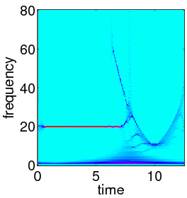
Figure 6: Revisiting the toy example from the Introduction. Left: the toy signal used for Figures 1 and 2; Middle: its instantaneous frequency; Right: the result of synchrosqueezing for this signal. The “extra” component at very low frequency is due to the signal’s not being centered around 0.

We next explore the tolerance to noise of synchrosqueezed wavelet transforms. We denote by $X(t)$ a white noise with zero mean and variance $\sigma^{2}=1$. The Signal-to-Noise Ratio (SNR) (measured in dB), will be defined (as usual) by

$$\text{SNR [dB]}=10\log_{10}\left(\frac{\operatorname{Var}f}{\sigma^{2}}\right),$$

where $f$ is the noiseless signal.

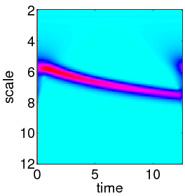
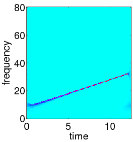
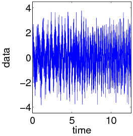
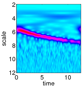
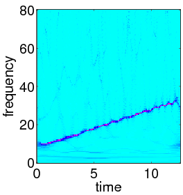
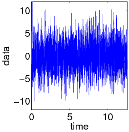
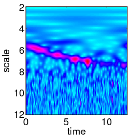
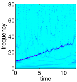
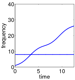
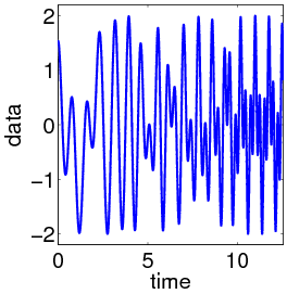
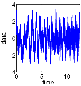
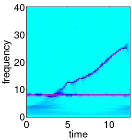
Figure 7: Top row: left: single chirp signal without noise; middle: its continuous wavelet transform, and right: the synchrosqueezed transform. Middle row: same, after white noise with SNR of $-3.00$ dB was added to the chirp signal.Lower row: same, now with white noise with SNR of $-12.55$ dB.

Figure 8: Far left: the instantaneous frequencies, $\omega(t)=2t+1-\sin(t)$ and $8$, of the the two IMT components of the crossover signal $f(t)=\cos[t^{2}+t+\cos(t)]+\cos(8t)$; Middle left: plot of $f(t)$ with no noise added; Middle: Synchrosqueezed wavelet transforms of noiseless $f(t)$; Middle right: $f(t)+$noise (corresponding to SNR of $6.45$ dB); Far right: synchrosqueezed wavelet transforms of $f(t)+$noise.

Figure 8 shows the results of applying our algorithm to a signal consisting of one single chirp function $f(t)=\cos(8t+t^{2})$, without noise (i.e. the signal is just $f$), with some noise (the signal is $f+X$, SNR$=-3.00$ dB), and with more noise($f+3X$, SNR$=-12.55$dB). Despite the high noise levels, the synchrosqueezing algorithm identifies the component with reasonable accuracy. Figure 10 below shows the instantaneous frequency curve extracted from these synchrosqueezed transforms, for the three cases.

Finally we try out a “crossover signal”, that is, a signal composed of two components with instantaneous frequency trajectories that intersect; in our example $f(t)=\cos(t^{2}+t+\cos(t))+\cos(8t)$. Figure 8 shows the signals $f(t)$ and $f(t)+0.5X(t)$, together with their synchrosqueezed wavelet transforms, as well as the “ideal” frequency profile given by the instantaneous frequencies of the two components of $f$.

5.2 Extracting Individual Components from Synthesized data

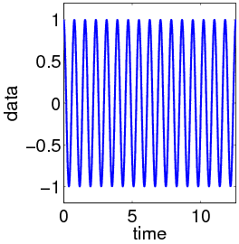
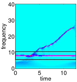
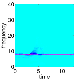
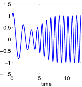
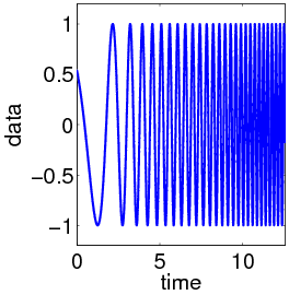
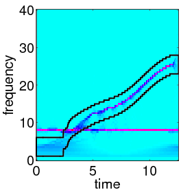
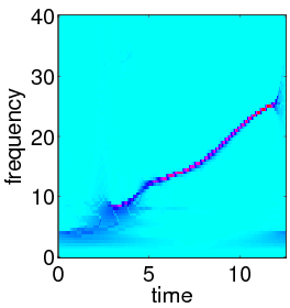
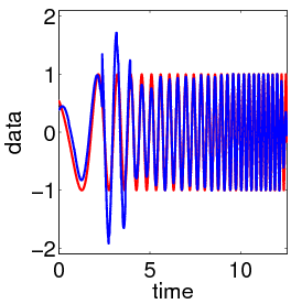
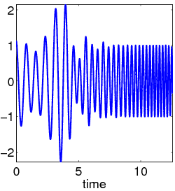
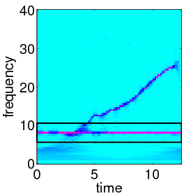
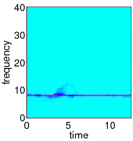
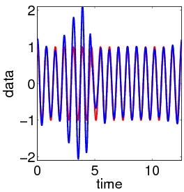
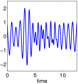
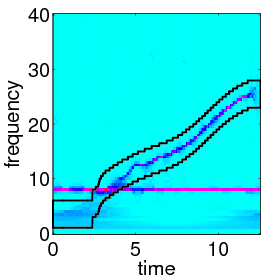
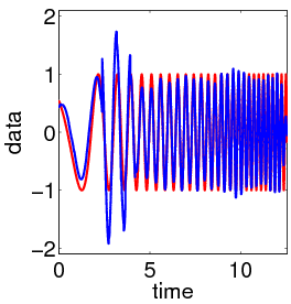
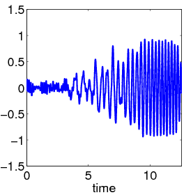
Figure 9: Comparing the decomposition into components $s_{1}(t)$ and $s_{2}(t)$ of the crossover signal $s(t)=s_{1}(t)+s_{2}(t)=\cos(8t)+\cos[t^{2}+t+\cos(t)]$ Rows: Noise-free situation in the first two rows; in the last two rows noise with SNR = $6.45$ dB was added to the mixed signal. In each case, $s_{1}$ is in the top row, and $s_{2}$ underneath. Columns: Far left: true $s_{j}(t)$ $j=1,2$; Middle left: Zone marked on the synchrosqueezed transform for reconstruction of the component; Center: part of the synchrosqueezed transform singled out for the reconstruction of a putative $s_{j}$; Middle Right: the corresponding candidate $s_{j}(t)$ according to the synchrosqueezed transform (plotted in blue over the original $s_{j}$, in red); Far right: candidate $s_{j}$ according to EMD in the noiseless case, EEMD in the noisy case.

In many applications listed in [5, 6, 11, 12, 18], the desired end goal is the instantaneous frequency trajectory or profile for the different components. When this is the case, the result of the synchrosqueezed wavelet transform, as illustrated in the preceding subsection, provides a solution.

In other applications, however, one may wish to consider the individual components themselves. These are obtained as an intermediary result, before extracting instantaneous frequency profiles, in the EMD and EEMD approaches. With synchrosqueezing, they can be obtained in an additional step after the frequency profiles have been determined.

Recall that, like most linear TF representations, the wavelet transform comes equipped with reconstruction formulas,

$$f(t) = C_{\psi}\,\int_{-\infty}^{\infty}\int_{0}^{\infty}W_{f}(a,b)\,a^{-5/2}\,\psi\left(\frac{t-b}{a}\right)\,\,\mathrm{d}a\,\mathrm{d}b~{},$$ (5.1)

$$\mbox{as well as }f(t) = C^{\prime}_{\psi}\,\int_{0}^{\infty}W_{f}(a,t)\,a^{-3/2}\,\,\mathrm{d}a=C^{\prime}_{\psi}\,\mathfrak{Re}\left[\,\int_{0}^{\infty}T_{f}(t,\omega)\,\mathrm{d}\omega\,\right],$$ (5.2)

where $C_{\psi},\,C^{\prime}_{\psi}$ are constants depending only on $\psi$. For the signals of interest to us here, the synchrosqueezed representation has, as illustrated in the preceding subsection, well localized zones of concentration. One can use these to select the zone corresponding to one component, and then integrate, in the reconstruction formulas, over the corresponding subregion of the integration domain. In practice, it turns out that the best results are obtained by using the reconstruction formula (5.1).

We illustrate this with the crossover example from the previous subsection: Figure 9 shows the zones selected in the synchrosqueezed transform plane as well as the corresponding reconstructed components. This figure also shows the components obtained for these signals by EMD for the clean case, and by EEMD (more robust to noise than EMD) for the noisy case; for this type of signal, the synchrosqueezed transform proposed here seems to give a more easily interpretable result.

Once the individual components are extracted, one can use them to get a numerical estimate for the variation in time of the instantaneous frequencies of the different components. To illustrate this, we revisit the chirp signal from the previous subsection. Figure 10 shows the frequency curves obtained by the synchrosqueezing approach; they are fairly robust with respect to noise.

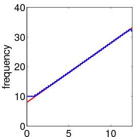
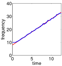
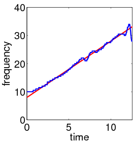
Figure 10: Instantaneous frequency curves extracted from the synchrosqueezed representation Left: the instantaneous frequency of the clean single chirp signal estimated by synchrosqueezing; Middle: the instantaneous frequency of the fairly noisy single chirp signal (SNR=$-3.00$dB) estimated by synchrosqueezing. Right:the instantaneous frequency of the noisy single chirp signal (SNR=$-12.55$dB) estimated by synchrosqueezing.

5.3 Applying the synchrosqueezed transform to some real data

So far, all the examples shown concerned toy models or synthesized data. In the subsection we illustrate the result on some real data sets, of medical origin.

5.3.A  Surface Electromyography Data

In this application, we “clean up” surface electromyography (sEMG) data acquired from a healthy young female with a portable system (QuickAmp). The sEMG electrodes, with sensors of high-purity sintered Ag/AgCl, were placed on the triceps. The signal was measured for 608 seconds, sampled at 500Hz. During the data acquisition, the subject flexed/extended her elbow, according to a protocol in which instructions to flex the right or left elbow were given to the subject at not completely regular time intervals; the subject did not know prior to each instruction which elbow she would be told to flex, and the sequence of left/right choices was random. The raw sEMG data $s_{l}(t)$ and $s_{r}(t)$ are shown in the left column in Figure 11.

    

 

 

 

 

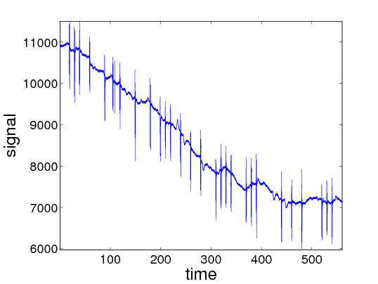
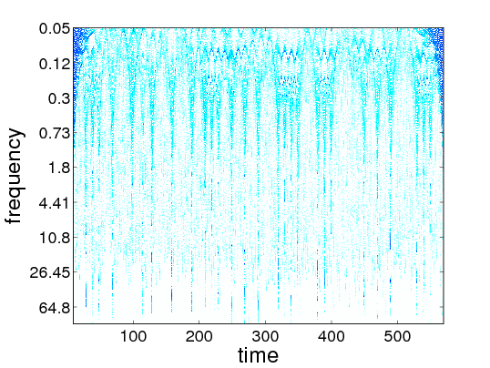
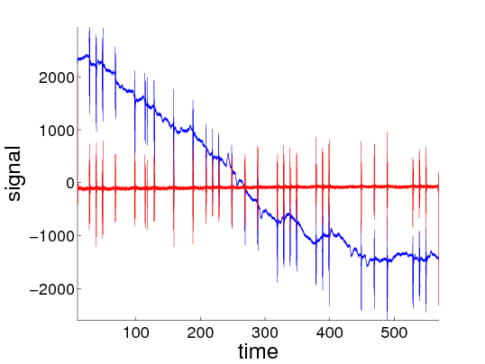
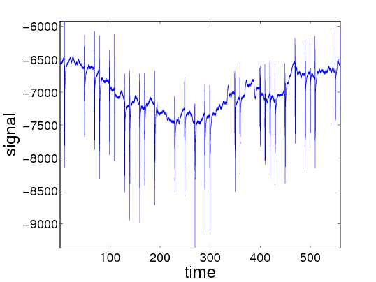
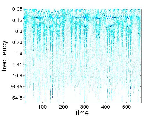
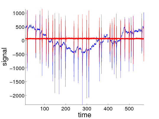
Figure 11: Left column: The surface electromyography data described in the text. The erratic (and different) drifts present in these signals are pretty typical. The very short-lived peaks correspond to the elbow-flexes by the subject. Note that the peaks have, on average, the same amplitudes for the left and right triceps; they look larger for the right triceps only because of a difference in scale. Middle column: The synchrosqueezing transforms of the surface electromyography signals. Coarse scales are near the top of these diagrams, finer scales are shown lower. The peaks are clearly marked over a range of fine scales. Right column: The red curve give the signals “sans drift”, reconstructed by deleting the low frequency region in the synchrosqueezed transforms; comparison with the original sEMG signals (in blue) shows the R peaks are as sharp as in the original signals, and at precisely the same location.

The middle column in Figure 11 shows the results $\mathcal{W}s_{\ell}(t,\omega)$, $\mathcal{W}s_{r}(t,\omega)$ of our synchrosqueezing algorithm applied to the two sEMG data sets. We used an implementation in which each dyadic scale interval ($a\in[2^{k},2^{k+1}]$) was divided into 32 equi-log-spaced bins.

The original surface electromyography signals show an erratic drift, which medical researchers wish to remove without losing any sharpness in the peaks. To achieve this, we identified the low frequency components (i.e. the dominant components at frequencies below 1 Hz) in the signal, and removed them before reconstruction. More, precisely, we defined $\widetilde{s}_{i}(t)=\sum_{\xi\geq\xi_{i,\mbox{\tiny{cut-off}}}}\mathcal{T}s_{i}(t,\xi)$, with frequency cut-off $\xi_{i,\mbox{\footnotesize{cut-off}}}(t)=\omega_{i}(t)+\omega_{0}$, where $\omega_{i}(t)$ was the dominant component for signal $i$ ($i=\ell$ or $r$) near 1 Hz with the highest frequency, and $\omega_{0}$ a small constant offset. The right column in Figure 11 shows the results; the erratic drift has disappeared and the peaks are well preserved. Note that a similar result can also be obtained straightforwardly from a wavelet transform without any synchrosqueezing.

5.3.B. Electrocardiogram Data

In this application we use synchrosqueezing to extract the heart rate variability (HRV) from a real electrocardiogram (ECG) signal. The data was acquired from a resting healthy male with a portable ECG machine at sampling rate $1000$Hz for $600$ seconds. The samples were quantized at $12$ bits across $\pm 10$ mV. The raw ECG data $e(t)$ are (partially) shown in the left half of Figure 12; the right half of the figure shows a blow-up of 20 seconds of the same signal.

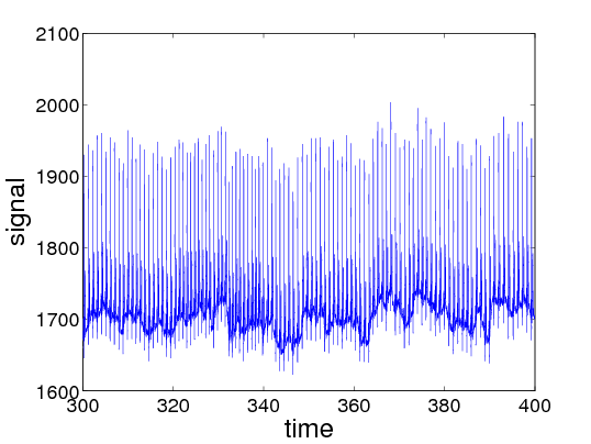
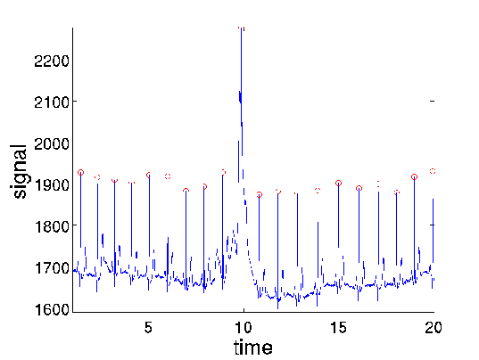
Figure 12: The raw electrocardiogram data Left: portion between 300 and 400 sec; Right: blow-up of the stretch between 320 and 340 sec, with the R peaks marked.

The strong, fairly regular spikes in the ECG are called the R peaks; the heart rate variability (HRV) time series is defined as the sequence of time differences between consecutive R peaks. (The interval between two consecutive R peaks is also called the RR interval.) The HRV is important for both clinical and basic research; it reflects the physiological dynamics and state of health of the subject. (See, e.g., [15] for clinical guidelines pertaining to the HRV, and [2] recent advances made in research.) The HRV can be viewed as a succession of snapshots of an averaged version of the instantaneous heart rate.

The left half of Figure 13 shows the synchrosqueezed transform $T_{e}(\omega,t)$ of $e(t)$; in this case we used an implementation in which each dyadic scale interval ($a\in[2^{k},2^{k+1}]$) was divided into $128$ equi-log-spaced bins. The synchrosqueezed transform $T_{e}(\omega,t)$ has a dominant line $c(t)$ near $1.2$Hz, the support of which can be parametrized as $\{(t,\omega_{c}(t));\,t\in[0,80\mbox{sec}]\,\}$. The right half of Figure 13 tracks the dependence on $t$ of $\omega_{c}(t)$. This figure also plot a (piecewise constant) function $f(t)$ that tracks the HRV time series and that is computed as follows: if $t$ lies between $t-i$ and $t_{i+1}$, the locations in time for the $i$-th and $(i+1)$-st R peaks, then $f(t)=[t_{i+1}-t_{i}]^{-1}$. The plot for $\omega(t)$ and $f(t)$ are clearly highly correlated.

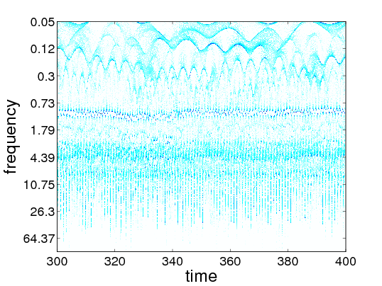
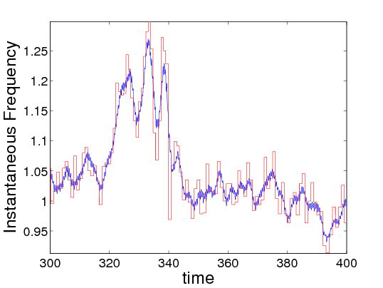
Figure 13: Left: The synchrosqueezing transforms of the electrocardiogram signals given in Fig. 12. Right: The blue curve shows the “instantaneous heart rate” $\omega(t)$ computed by tracking the support of the dominant curve in the synchrosqueezed transform $T_{e}$; the red curve is the (piecewise constant) inverse of the successive $\mbox{RR}_{i}$

6 Acknowledgments

The authors are grateful to the Federal Highway Administration, which supported this research via FHWA grant DTFH61-08-C-00028. They also thank Prof. Norden Huang and Prof. Zhaohua Wu for many stimulating discussions and their generosity in sharing their code and insights. They also thank MD. Shu-Shya Hseu and Prof. Yu-Te Wu for providing the real medical signal.

References

• [1] F. Auger and P. Flandrin, Improving the readability of time-frequency and time-scale representations by the reassignment method, IEEE Trans. Signal Process. 43 (1995), no. 5, 1068–1089.
• [2] S. Cerutti, A.L. Goldberger, and Y. Yamamoto, Recent advances in heart rate variability signal processing and interpretation, Biomedical Engineering, IEEE Transactions on 53 (2006), no. 1, 1–3.
• [3] E. Chassande-Mottin, F. Auger, and P. Flandrin, Time-frequency/time-scale reassignment, Wavelets and signal processing, Appl. Numer. Harmon. Anal., Birkhäuser Boston, Boston, MA, 2003, pp. 233–267.
• [4] E. Chassande-Mottin, I. Daubechies, F. Auger, and P. Flandrin, Differential reassignment, Signal Processing Letters, IEEE 4 (1997), no. 10, 293–294.
• [5] M. Costa, A. A. Priplata, L. A. Lipsitz, Z. Wu, N. E. Huang, A. L. Goldberger, and C.-K. Peng, Noise and poise: Enhancement of postural complexity in the elderly with a stochastic-resonance-based therapy, Europhys. Lett. 77 (2007), 68008.
• [6] D. A. Cummings, R. A. Irizarry, N. E. Huang, T. P. Endy, A. Nisalak, K. Ungchusak, and D. S. Burke, Travelling waves in the occurrence of dengue haemorrhagic fever in Thailand, Nature 427 (2004), 344–347.
• [7] I. Daubechies and S. Maes, A nonlinear squeezing of the continuous wavelet transform based on auditory nerve models, Wavelets in Medicine and Biology (A. Aldroubi and M. Unser, eds.), CRC Press, 1996, pp. 527–546.
• [8] P. Flandrin, Time-frequency/time-scale analysis, Wavelet Analysis and its Applications, vol. 10, Academic Press Inc., San Diego, CA, 1999, With a preface by Yves Meyer, Translated from the French by Joachim Stöckler.
• [9] P. Flandrin, G. Rilling, and P. Goncalves, Empirical mode decomposition as a filter bank, IEEE Signal Process. Lett. 11 (2004), no. 2, 112–114.
• [10] C. Huang, L. Yang, and Y. Wang, Convergence of a convolution-filtering-based algorithm for empirical mode decomposition, Advances in Adaptive Data Analysis 1 (2009), 560–571.
• [11] N. E. Huang, Z. Shen, S. R. Long, M. C. Wu, H. H. Shih, Q. Zheng, N.-C. Yen, C. C. Tung, and H. H. Liu, The empirical mode decomposition and the hilbert spectrum for nonlinear and non-stationary time series analysis, Proc. R. Soc. A 454 (1998), 903–995.
• [12] N. E. Huang and Z. Wu, A review on hilbert-huang transform: Method and its applications to geophysical studies, Rev. Geophys. 46 (2008), RG2006.
• [13] N. E. Huang, Z. Wu, S. R. Long, K. C. Arnold, K. Blank, and T. W. Liu, On instantaneous frequency, Advances in Adaptive Data Analysis 1 (2009), 177–229.
• [14] L. Lin, Y. Wang, and H. Zhou, Iterative filtering as an alternative algorithm for empirical mode decomposition, Advances in Adaptive Data Analysis 1 (2009), 543–560.
• [15] M. Malik and A. J. Camm, Dynamic electrocardiography, Wiley, 2004.
• [16] G. Rilling and P. Flandrin, One or two frequencies? the empirical mode decomposition answers, IEEE Trans. Signal Process. 56 (2008), no. 1, 85–95.
• [17] Z. Wu and N. E. Huang, A study of the characteristics of white noise using the empirical mode decomposition method, Proc. R. Soc. A 460 (2004), 1597–1611.
• [18]  , Ensemble empirical mode decomposition: A noise-assisted data analysis method, Advances in Adaptive Data Analysis 1 (2009), 1–41.