Extended Self Similarity works for the Burgers equation and why

Abstract

Extended Self-Similarity (ESS), a procedure that remarkably extends the range of scaling for structure functions in Navier–Stokes turbulence and thus allows improved determination of intermittency exponents, has never been fully explained. We show that ESS applies to Burgers turbulence at high Reynolds numbers and we give the theoretical explanation of the numerically observed improved scaling at both the infrared and ultraviolet end, in total a gain of about three quarters of a decade: there is a reduction of subdominant contributions to scaling when going from the standard structure function representation to the ESS representation. We conjecture that a similar situation holds for three-dimensional incompressible turbulence and suggest ways of capturing subdominant contributions to scaling.

1 Introduction

Extended Self-Similarity (ESS), discovered by Benzi et al. (1993), is the empirical observation that in fully developed turbulence, when plotting structure functions of order $p$ vs, say, the structure function of order three, rather than the traditional way where they are plotted vs the separation, then the range over which clean power-law scaling is observed can be substantially increased. This has allowed a much better determination of the scaling exponents $\zeta_{p}$ of the structure functions of order $p$ — or at least of ratios of such exponents — and has been key to confirming that three-dimensional high Reynolds number incompressible turbulence does not follow the Kolmogorov (1941) scaling laws $\zeta_{p}=p/3$, but instead has anomalous scaling, whose exponents cannot be obtained solely through dimensional arguments.

In spite of several attempts to explain the success of ESS (see, e.g. Bhattacharjee & Sain, 1999; Sain & Bhattacharjee, 1999; Fujisaka & Grossmann, 2001; Segel et al., 1996; Yakhot, 2001, and Section 5), the latter is still not fully understood and we do not know how much we can trust scaling exponents derived by ESS. It would be nice to have at least one instance for which ESS not only works, but does so for reasons we can rationally understand. A very natural candidate might be the one-dimensional Burgers equation. Early attempts to test ESS on the Burgers equation did not show any appreciable increase in the quality of scaling through the use of ESS. As we shall see in Section 3, the conclusion that “ESS does not work for the Burgers equation” Benzi et al. (1995) was just reflecting the computational limitations of the early nineties.

In Section 2 we recall some basic facts and notation for ESS in three-dimensional Navier–Stokes turbulence. Then in Section 3 we turn to the Burgers equation and present new numerical evidence that ESS works for Burgers, provided high enough spatial resolution is used. In Section 4 we use asymptotic theory to explain in detail why ESS works for the Burgers case. Finally, in Section 5 we examine the possible lessons from our Burgers ESS study for three-dimensional Navier–Stokes turbulence.

2 ESS in a nutshell

Consider the three-dimensional Navier–Stokes (3DNS) equation

$$\partial_{t}{\bf v}+{\bf v}\cdot\nabla{\bf v}=-\nabla p+\nu\nabla^{2}{\bf v},\qquad\nabla\cdot{\bf v}=0.$$ (1)

For the case of homogeneous isotropic turbulence, (longitudinal) structure functions of integer order $p$ are defined as

$$S_{p}(r)\equiv\left\langle\left(\delta v_{\parallel}({\bf r})\right)^{p}\right\rangle,$$ (2)

in terms of the longitudinal velocity increments

$$\delta v_{\parallel}({\bf r})\equiv[{\bf v}({\bf x}+{\bf r})-{\bf v}({\bf x})]\cdot\frac{{\bf r}}{r}\,,$$ (3)

where $r\equiv|{\bf r}|$ and the angular brackets denote averaging. There is experimental and numerical evidence that, at high Reynolds numbers, structure functions follow scaling laws (see. e.g. Monin & Yaglom, 1971; Frisch, 1995)

$$S_{p}(r)\propto r^{\zeta_{p}}$$ (4)

over some range of separations (the inertial range) $L\gg r\gg\eta_{p}$. Here $L$ is the integral scale and $\eta_{p}$ the dissipation scale. The latter may depend on the order $p$ (see e.g. Paladin & Vulpiani, 1987; Frisch & Vergassola, 1991).

Of course, the dominant-order behaviour given by (4) is accompanied by subdominant corrections involving the two small parameters characteristic of inertial-range intermediate asymptotics, namely $r/L$ and $\eta_{p}/r$. The simplest would be to have

$$S_{p}(r)=C_{p}r^{\zeta_{p}}\left(1+D_{p}^{\rm IR}(r/L)^{g_{p}^{\scriptscriptstyle\rm IR}}+D_{p}^{\rm UV}(\eta_{p}/r)^{g_{p}^{\scriptscriptstyle\rm UV}}\right)+{\rm h.o.t.}\,,$$ (5)

where h.o.t. stands for “higher-order terms” and where $g_{p}^{\rm IR}>0$ and $g_{p}^{\rm UV}>0$ are the infrared (IR) and ultraviolet (UV) gaps, respectively. For a given Reynolds number and thus a given ratio $L/\eta_{p}$, the smaller the gaps and the constants $D_{p}^{\rm IR}$ and $D_{p}^{\rm UV}$, the larger the range of separations over which subdominant corrections remain small.

The ESS is an operational procedure that effectively enlarges the range of separations over which dominant-order scaling is a good approximation. In its simplest formulation, one considers two integer orders $n$ and $m$ and plots $|S_{n}(r)|$ vs $|S_{m}(r)|$ and finds empirically that the scaling relations

$$|S_{n}(r)|\approx|S_{m}(r)|^{\alpha(n,m)}\,,$$ (6)

with suitable exponents $\alpha(n,m)$, hold much better than (4). One particularly interesting instance of this procedure is when $m=3$. We then know from Kolmogorov (1941) that, to dominant order, we have the four-fifths law (see, also Frisch, 1995)

$$S_{3}(r)=-\frac{4}{5}\varepsilon r\,,$$ (7)

where $\varepsilon$ is the mean energy dissipation per unit mass. Thus, the third-order structure function (divided by $-(4/5)\varepsilon$) may be viewed as a deputy of the separation $r$. A variant of the ESS, which frequently gives even better scaling, is to use alternative structure functions, defined with the absolute values of the longitudinal velocity increments, namely

$$F_{p}(r)\equiv\left\langle\left|\delta v_{\parallel}({\bf r})\right|^{p}\right\rangle\,.$$ (8)

It is then found empirically that

$$F_{n}(r)\approx F_{m}(r)^{\beta(n,m)}\,,$$ (9)

with suitable scaling exponents $\beta(n,m)$. Whatever its empirical merits, the variant procedure has the drawback that there is no equivalent to the four-fifths law for the third-order structure function with the absolute value of the longitudinal velocity increment. Thus we cannot safely use $F_{3}(r)$ as a deputy of $r$. We shall come back to this in Section 5.

3 ESS revisited for the Burgers equation

The one-dimensional Burgers equation

$$\partial_{t}u+u\partial_{x}u=\nu\partial_{x}^{2}u;\quad u(x,0)=u_{0}(x),$$ (10)

which was introduced originally as a kind of poor man’s Navier–Stokes equation (see, e.g., Burgers, 1974), has some dramatic differences with three-dimensional Navier–Stokes (3DNS) turbulence, foremost that it is integrable Hopf (1950); Cole (1951) and — as a consequence — does not display self-generated chaotic behaviour. Nevertheless it does display anomalous scaling in the following sense: superficially, the Kolmogorov (1941) theory is applicable to the Burgers equation as much as it is to 3DNS. However, when starting with smooth initial data $u_{0}(x)$, the evolved solution in the limit of vanishing viscosity $\nu$ will display shocks. Thus $\zeta_{p}=1$ for $p\geq 1$. When the Reynolds number is finite, structure functions will display scaling only over a limited range of separations $r$. Therefore, the Burgers equation may be a good testing ground for ESS and also perhaps for understanding why and when it works. Such considerations did not escape the creators of the ESS technique. Unfortunately, no clean scaling for structure functions is observed with the Burgers equation, either in the standard representation or in ESS, as long as simulations are done with the spatial resolution easily available in the early nineties, namely a few thousand collocation points. Scaling emerges only at much higher spatial resolutions with 128K ($128\times 1024$) Fourier modes and becomes fully manifest with 256K modes, which is now also the highest resolution achievable numerically within a time span of a few week.

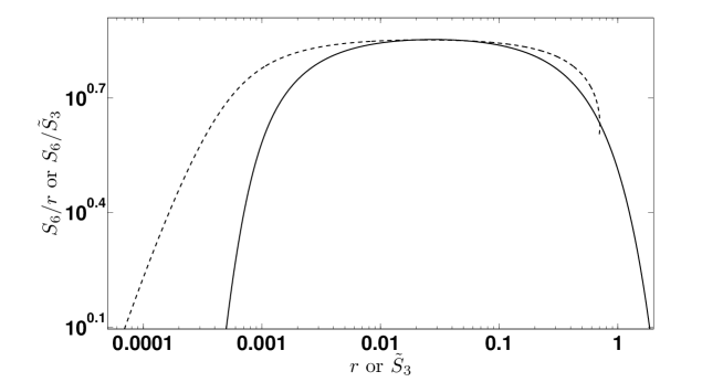
Figure 1: Compensated sixth-order structure function in standard (continuous line) and ESS (dashed line) representations.

Let us now explain our numerical strategy for studying ESS with the Burgers equation. Our goal in doing preliminary numerical experiments is to understand ESS in a rational way, starting from the basic equations. For this it is advisable to keep the formulation minimally complex, avoiding too many “realistic trappings”. For example, there is no need at first to assume random initial conditions: we can just take an $L$-periodic initial condition and define the structure functions by integrating over the period:

$$S_{p}(r)\equiv(1/L)\int_{0}^{L}dx\,[u(x+r,t)-u(x,t)]^{p}.$$ (11)

We shall mostly work with a very simple single-mode model for which the initial condition is $2\pi$-periodic deterministic and has a single Fourier mode

$$u_{0}=\sin x.$$ (12)

As we shall see in Section 4, it is easy to extend the theory from the deterministic to the random case.

We integrated the Burgers equation (10) with the initial condition (12) using a pseudo-spectral method with $N$ collocation points and a two-thirds alias-removal rule. Time stepping was done in double precision by a 4th order Runge–Kutta scheme with constant time step $\delta t$. The viscous term was handled by the slaving technique known as ETDRK4 described in Cox & Matthews (2002), which allows taking a time step about ten times larger than would be permitted with a direct handling of the viscous term. (It was pointed out by Kassam & Trefethen (2005) that ETDRK4 can produce numerically ill-conditioned cancellations; following a suggestion of J.Z. Zhu (private communication), we handled these by performing Taylor expansions to suitable order rather then by the complex-plane method proposed by Kassam & Trefethen (2005).) Slaving results not only in considerable speed-up but in much less accumulation of rounding noise.

The parameters of the run were $N=256K$ and $\delta t=10^{-5}$. Output was processed at $t=2$, well beyond the time of appearance of the first shock at $t=t_{\star}=1$ .

Fig. 1 shows the compensated structure function — that is divided by the theoretically predicted inertial-range dominant term — of order six in both the standard representation and in a variant of the ESS representation. Our variant uses

$$\tilde{S}_{3}(r)\equiv\frac{S_{3}(r)}{-12\varepsilon},$$ (13)

where $\varepsilon\equiv-(1/L)(d/dt)\int_{0}^{L}dx\,u^{2}/2$ is the mean energy dissipation. It is easy to show that the Burgers counterpart of the four-fifth low is a “minus twelve” law (cf. Gurbatov et al., 1997) which makes $\tilde{S}_{3}$ the appropriate deputy of the separation $r$. In our opinion it is important to chose the constant in the definition of $\tilde{S}_{3}$ in such a way that it becomes $r$ with a unit factor (to dominant order). Otherwise an ESS plot in log-log coordinates may show an overall improvement in quality of scaling, without our being able to disentangle the small-separation (UV) improvement from the large-separation (IR) improvement. As we shall see, both are in general present and have quite different origins.

Fig. 1 shows a substantial improvement in scaling for ESS, that is a wider horizontal plateau in the compensated structure function; and this at both the IR and UV ends. This is the first evidence that “ESS works for Burgers”. Next we shall understand why it works.

4 Asymptotic theory of ESS for the Burgers equation

We now give the theory for improved ESS scaling when $p\geq 3$, first for the single mode case and then upgrade it for the case of random solutions.

To handle the infrared (IR) contributions to the structure functions we can work with an infinitely sharp shock, taking $\nu\to 0$. The dominant contribution to structure functions of integer order comes clearly from intervals $[x,\,x+r]$ which straddle the shock location $x_{\scriptscriptstyle\rm S}$ (in this Section the time variable is written explicitly only when needed). It is also easily shown that for $p\geq 3$ the first-order subdominant contributions comes from the small changes of the velocity, immediately to the left and the right of the shock, which are expressible by Taylor expanding the velocity to first order in these two regions (see Section 4.2.2 of Bec et al., 2000):

$$u(x)=u_{-}+(x-x_{\scriptscriptstyle\rm S})s_{-}+\textrm{h.o.t.},\quad u(x)=u_{+}+(x-x_{\scriptscriptstyle\rm S})s_{+}+\textrm{h.o.t.},$$ (14)

where $u_{-}$ and $u_{+}$ are the velocities immediately to the left and to the right of the shock and $s_{-}$ and $s_{+}$ their respective gradients. Starting from (11) and limiting the integration domain to the interval $[x_{\scriptscriptstyle\rm S}-r,\,x_{\scriptscriptstyle\rm S}]$, which corresponds to the straddling condition, we obtain, using (14)

$$LS_{p}(r)=(-1)^{p}\left(\Delta^{p}r-\Delta^{p-1}(s_{+}+s_{-})\frac{p}{2}r^{2}\right)+\textrm{h.o.t.},$$ (15)

where

$$\Delta\equiv u_{-}-u_{+}>0$$ (16)

is the amplitude of the shock and $L=2\pi$ is the spatial period. Specialising to the third-order structure function and to its rescaled version the separation deputy $\tilde{S}_{3}(r)\equiv S_{3}(r)/(-12\varepsilon)$, we obtain

$$LS_{3}(r) = -\Delta^{3}r+\left(\frac{3}{2}\right)\Delta^{2}(s_{-}+s_{+})r^{2}+\textrm{h.o.t.}$$ (17)

$$\tilde{S}_{3}(r) = r-\left(\frac{3}{2\Delta}\right)(s_{-}+s_{+})r^{2}+\textrm{h.o.t.},$$ (18)

where we have used the relation

$$\varepsilon=\frac{\Delta^{3}}{12L}$$ (19)

between the energy dissipation and the shock strength.

We now eliminate $r$ between (18) and (15), so a to rewrite the structure function of order $p$ as an expansion in the separation deputy :

$$LS_{p}=(-1)^{p}\left(\Delta^{p}\tilde{S}_{3}-\Delta^{p-1}\left(\frac{p-3}{2}\right)(s_{-}+s_{+})\tilde{S}_{3}^{2}\right)+\textrm{h.o.t.}$$ (20)

Comparison of the “standard” expansion (15) of the structure function and its ESS expansion (20), shows that they have the same dominant terms and that their first subdominant corrections differ only by a numerical coefficient: $p/2$ for the standard case and $(p-3)/2$ for ESS. Hence the subdominant correction has been decreased by a factor $p/(p-3)$. For the case of the sixth-order structure function, considered in Fig. 1, this is a reduction by a factor two. Hence, the ESS inertial-range scaling extends by a factor $2$ further into the IR direction before a same level of degradation is achieved as for the standard case. Note that for large $p$s the gain in scaling range becomes smaller.

Next we turn to the ultraviolet (UV) contributions which now require a finite viscosity $\nu$ that broadens the shock. Standard boundary layer analysis for the shock in the frame where the shock is at rest (which basically amounts to dropping the time derivative term in the Burgers equation) gives the following well-known tanh structure :

$$u(x)\approx-\frac{\Delta}{2}\tanh\frac{x\Delta}{4\nu}.$$ (21)

Hence the UV structure functions are given by

$$LS_{p}(r)=\left(\frac{\Delta}{2}\right)^{p}\int_{-\infty}^{\infty}dx\left[\tanh\frac{x\Delta}{4\nu}-\tanh\frac{(x+r)\Delta}{4\nu}\right]^{p}.$$ (22)

We are interested in the expansion of these structure functions for $r$ much larger than the typical width $4\nu/\Delta$ of the shock. For this, we first established the following expansion (for large $\tilde{r}$)

$$\int_{-\infty}^{\infty}d\tilde{x}\,[\tanh(\tilde{x})-\tanh(\tilde{x}+\tilde{r})]^{p}=(-2)^{p}(\tilde{r}-H_{p-1})+\textrm{t.s.t.}$$ (23)

where “t.s.t.” stands for “transcendentally small terms” such as $\exp(-\tilde{r})$ and
$H_{p}\equiv 1+1/2+1/3+...+1/p$ is the Harmonic function, which behaves as $\ln p$ for large $p$. Using (24) in (22), we obtain

$$LS_{p}(r)=(-1)^{p}\left(\Delta^{p}r-4\nu H_{p-1}\Delta^{p-1}\right)+\textrm{t.s.t.}$$ (24)

Specialising to $p=3$, we have

$$LS_{3}=-\Delta^{3}r+6\nu\Delta^{2}+\textrm{t.s.t.},\quad\tilde{S}_{3}(r)=r-6\frac{\nu}{\Delta}+\textrm{t.s.t.}.$$ (25)

Proceeding as in the IR case, we re-expand $S_{p}$ in terms of the deputy separation $\tilde{S}_{3}$:

$$LS_{p}(r)=(-1)^{p}\left(\tilde{S}_{3}\Delta^{p}-4\nu\left(H_{p-1}-\frac{3}{2}\right)\Delta^{p-1}\right)+\textrm{t.s.t.}$$ (26)

Thus, we see that with ESS the subdominant UV term for the structure function of order $p$ is reduced by a factor $2H_{p-1}/(2H_{p-1}-3)$ and, again, the range of scaling is extended by the same factor. For $p=6$ the extension factor is $137/47\approx 2.91$. Combining the UV and the IR gains, we see that the scaling for $S_{6}$ is extended by a factor $5.92$, that is about three quarters of a decade.

Next we upgrade the arguments to the case of the Burgers equation with smooth random initial conditions and forcing, defined on the whole real line. We assume that the forces and the initial conditions are (statistical) homogeneous and have rapidly decreasing spatial correlations (mixing). We can then use ergodicity to obtain the following representation of structure functions:

$$S_{p}(r)\equiv\langle\left(u(x+r)-u(x)\right)^{p}\rangle=\lim_{L\to\infty}\frac{1}{L}\int_{0}^{L}dx\,\left(u(x+r)-u(x)\right)^{p},$$ (27)

where the limit is in the almost sure sense. In the present context we have typically an infinite number of shocks on the whole line, but a finite number per unit length. The shock amplitudes $\Delta$ and the left and right velocity gradients $s_{-}$ and $s_{+}$ become random variables. Revisiting the arguments given above for the deterministic single-mode case, we find that in both the IR and UV expansions we now have to add the contributions stemming from the various shocks. Using ergodicity we obtain, in the UV domain

$$S_{p}(r)=(-1)^{p}\left(\langle\Delta^{p}\rangle\,r-4\nu H_{p-1}\langle\Delta^{p-1}\rangle\right)+\textrm{t.s.t.}$$ (28)

and, in the IR domain

$$S_{p}(r) = (-1)^{p}\left(\langle\Delta^{p}\rangle\,r-\langle\Delta^{p-1}(s_{+}+s_{-})\rangle\,\frac{p}{2}r^{2}\right)+\textrm{h.o.t.}$$ (29)

In the UV case we now make use of the inequality ${\langle\Delta^{p}\rangle}/{\langle\Delta^{p-1}\rangle}\geq{\langle\Delta^{3}\rangle}/{\langle\Delta^{2}\rangle}$, which follows, for $p\geq 3$, from the log-convexity of the moment function $q\mapsto\ln\langle\Delta^{q}\rangle$ for a positive random variable $\Delta$. We can then finish the analysis of the depletion of subdominant contributions essentially as done above (in the UV) case and conclude that ESS extends the UV scaling by at least a factor $2H_{p-1}/(2H_{p-1}-3)$. In the IR domain, the presence of the random quantity $s_{+}+s_{-}$ prevents us from reaching similar conclusions and it is thus not clear that there is a general result regarding improved ESS scaling in the IR regime. This can however be circumvented, if we assume (i) that the Burgers turbulence is freely decaying (no forcing) and (ii) we limit ourselves to times large compared to the typical turnover time of the initial condition. The solution degenerates then into a set of ramps of slope exactly $1/t$, separated by shocks. Hence $s_{+}+s_{-}\approx 2/t$, which is deterministic. Thus, using the same log-convexity inequality as above we infer that ESS extends the IR scaling by at least a factor $p/(p-3)$.

5 Back to three-dimensional Navier–Stokes turbulence

Here, we have explained the success of ESS by a depletion of subdominant IR and UV contributions. How does this relate to various explanations given over the past one and half decade for 3DNS turbulence? Let us mention a few. Sain and Bhattacharjee (see, Bhattacharjee & Sain, 1999; Sain & Bhattacharjee, 1999) resorted to phenomenology in proposing cross-over functions from the dissipation- to the inertial-range for the structure functions defined in Fourier space. They inferred that in the UV regime, the linear scaling in log-log plots of structure function deteriorate at lower values of wavenumbers than in the corresponding ESS plots. Fujisaka & Grossmann (2001) — again phenomenologically — introduced a scaling variable to include crossovers between various subranges of scaling behaviour for the magnitude of longitudinal velocity differences and thereby showed that the scaling improves at the IR end when ESS is used. In the spirit of our formulation of a theory for ESS, the work of Segel et al. (1996) comes closest. In this paper they have correctly identified the mechanism of increased scaling range at the UV end: a reduced coefficient in the subdominant diffusive correction. Note that their work on ESS was in the context of intermittency and anomalous scaling for passive scalar dynamics. They used the model of Kraichnan (1968, 1994) and supplemented it by a closure relation suggested by Kraichnan (1994), which was later shown not to be fully consistent with the original model (see e.g., Falkovich et al., 2001). Benzi (private communication) also made a similar observation using a passive scalar shell model.

How much of our findings for the Burgers equation carry over to 3DNS? It is important to realize that the improved scaling can be both at the IR and the UV end of the scaling regime. In order to avoid mixing up the two types of improvements one should correctly calibrate the choice of the deputy for the separation $r$, by using the four-fifths law for 3DNS:

$$\tilde{S}_{3}(r)\equiv-\frac{S_{3}}{(4/5)\varepsilon}.$$ (30)

If a given turbulent flow shows a gain in scaling when using ESS, either in the IR or the UV domain or both, we can then use (5) to interpret the gain in terms of subdominant corrections. It is best to handle the IR and UV cases separately. Following the same procedure as in Section 4 it is easily shown that ESS gives just a modification of the coefficient of the first subdominant contribution provided the gap $g_{p}$ between dominant and first subdominant exponent is independent of the order $p$. The fact that ESS works so nicely for 3DNS suggests that this independence may actually hold. If so, it is immediately seen that the reduction in the subdominant coefficient is equal to the gain in scaling raised to the gap value.

We begin to see here ESS as a way to obtain information on subdominant corrections. This is of interest for several reasons. For example, subdominant corrections can give rise to spurious multifractal scaling (see e.g., Aurell et al., 1992; Mitra et al., 2005). Furthermore, consideration of subdominant corrections is needed to explain the absence of logarithms in the third-order structure function (cf. Frisch et al., 2005). Also, the multifractal description of turbulence is quite heuristic and arbitrary and would be much more strongly constrained if we had information on subdominant terms and on gap values.

This may be the right place to discuss the issue of the best deputy of separation in the ESS procedure. Should one use $S_{3}(r)$ or the function $F_{3}(r)$ that is defined with the third moment of the absolute value of the longitudinal velocity increment and which is easier to extract from experimental data because it involves only positive contributions? It is not clear to what extent the two procedures are equivalent. For the case of the Burgers turbulence it is easy to show that $-S_{3}(r)$ and $F_{3}(r)$ have the same dominant and first-order subdominant terms: they differ only in subsubdominant contributions. For 3DNS longitudinal velocity increments are somewhat more likely to be negative than positive but they have no reason to have exactly the same scaling behaviour although the scaling exponents are found to be nearly equal Vainshtein & Sreenivasan (1994). There has also been some amount of discussion regarding the scaling of longitudinal and transverse structure functions (see e.g., Benzi et al., 2009). It may well be that they differ only by the relative strength of subdominant terms.

We finally address the issue of appropriate strategies to systematically obtain subdominant corrections from experimental or simulation data. The most straightforward method is to determine the dominant-order contribution using ESS and then to subtract it from the the data. The result can then be analysed either in the standard way or in the ESS fashion. However it is known that when subdominant terms are rather sizeable it is better to determine them at the same time as the dominant ones. One instance is the simultaneous determination of dominant-order isotropic scaling and subdominant anisotropic corrections for weakly anisotropic turbulence (see e.g., Arad et al., 1998; Biferale & Procaccia, 2005, and references therein).

The determination of both dominant and subdominant terms can be much improved when higher precision is available, such as is frequently the case in double-precision spectral simulations. Indeed it was recently pointed out by van der Hoeven (2009) that, when trying to extract the asymptotic expansion of a function $f(x)$ as $x\to\infty$ from data sampled at a large number of values of discrete $x$-values, it not advisable to first try to obtain the dominant order and only then to look for subdominant terms: without the knowledge of subdominant corrections, the parameters appearing in the dominant term will be very poorly conditioned. It is better to completely subvert the dominant-order-first strategy by introducing the method of asymptotic interpolation, which relies on a series of transformations, recursively, peeling off the dominant and subdominant terms in the asymptotic expansion without any need to know their detailed functional form. These transformations can, in principle, be carried out till either the rounding noise becomes significant or asymptoticity is lost. At the end of the process, the newly transformed data admit a simple interpolation to — usually — a constant. Then by undoing the peeling-off transformations, one can determine very accurately the asymptotic expansion of the data up to a certain number of subdominant terms, which depends on the precision available on the original data. This method has been applied to various nonlinear problems and shown to give very accurate expression of the asymptotic expansion when the data have enough precision (see e.g., Pauls & Frisch, 2007; Bardos et al., 2009).