Representation of the three-body Coulomb Green’s function in parabolic coordinates: paths of integration

Abstract

The possibility is discussed of using straight-line paths of integration in computing the integral representation of the three-body Coulomb Green’s function. In our numerical examples two different integration contours are considered. It is demonstrated that only one of these straight-line paths provides that the integral representation is valid.

I Introduction

In two previous papers JP1 ; JP2 the method was introduced as a new approach for solution of the three-body continuum problem using infinite set of $L^{2}$ parabolic Sturmian basis functions for the wave function of the system. The goal of these papers has been the construction of exact analytic matrix elements of the three-body Coulomb Green’s function. The corresponding six-dimensional resolvent operator has been expressed as a convolution integral of three two-dimensional Green’s function. In this paper we wish to learn how to choose appropriate straight-line paths of integration which provide that the integral representation is valid.

Below we outline how the Schrödinger equation for a three-body Coulomb system is transformed into a Lippmann-Schwinger equation in terms of generalized parabolic coordinates.

The Schrödinger equation for three particles with masses $m_{1}$, $m_{1}$, $m_{3}$ and charges $Z_{1}$, $Z_{2}$, $Z_{3}$ is

$$\left[-\frac{1}{2\mu_{12}}\Delta_{\bf R}-\frac{1}{2\mu_{3}}\Delta_{\bf r}+\frac{Z_{1}Z_{2}}{r_{12}}+\frac{Z_{2}Z_{3}}{r_{23}}+\frac{Z_{1}Z_{3}}{r_{13}}\right]\Psi=E\Psi,$$ (1)

where ${\bf R}$ and ${\bf r}$ are the Jacobi vectors

$${\bf R}={\bf r}_{1}-{\bf r}_{2},\quad{\bf r}={\bf r}_{3}-\frac{m_{1}{\bf r}_{1}+m_{2}{\bf r}_{2}}{m_{1}+m_{2}},$$ (2)

${\bf r}_{ls}={\bf r}_{l}-{\bf r}_{s}$, $r_{ls}=\left|{\bf r}_{ls}\right|$, $\mu_{12}$ and $\mu_{3}$ are the reduced masses

$$\mu_{12}=\frac{m_{1}m_{2}}{m_{1}+m_{2}},\quad\mu_{3}=\frac{m_{3}\left(m_{1}+m_{2}\right)}{m_{1}+m_{2}+m_{3}}.$$ (3)

The ansatz

$$\Psi=e^{i({\bf K}\cdot{\bf R}+{\bf k}\cdot{\bf r})}\overline{\Psi}$$ (4)

removes the eigenenergy $E=\frac{1}{2\mu_{12}}\,{\bf K}^{2}+\frac{1}{2\mu_{3}}\,{\bf k}^{2}$ giving the equation for $\overline{\Psi}$

$$\left[-\frac{1}{2\mu_{12}}\,\Delta_{\bf R}-\frac{1}{2\mu_{3}}\,\Delta_{\bf r}-\frac{i}{\mu_{12}}\,{\bf K}\cdot\nabla_{\bf R}-\frac{i}{\mu_{3}}\,{\bf k}\cdot\nabla_{\bf r}+\frac{Z_{1}Z_{2}}{r_{12}}+\frac{Z_{2}Z_{3}}{r_{23}}+\frac{Z_{1}Z_{3}}{r_{13}}\right]\overline{\Psi}=0.$$ (5)

Then, the operator in the square braces is expressed in terms of the generalized parabolic coordinates Klar

$$\begin{array}[]{c}\xi_{1}=r_{23}+\hat{\bf k}_{23}\cdot{\bf r}_{23},\quad\eta_{1}=r_{23}-\hat{\bf k}_{23}\cdot{\bf r}_{23},\\ \xi_{2}=r_{13}+\hat{\bf k}_{13}\cdot{\bf r}_{13},\quad\eta_{2}=r_{13}-\hat{\bf k}_{13}\cdot{\bf r}_{13},\\ \xi_{3}=r_{12}+\hat{\bf k}_{12}\cdot{\bf r}_{12},\quad\eta_{3}=r_{12}-\hat{\bf k}_{12}\cdot{\bf r}_{12},\\ \end{array}$$ (6)

where ${\bf k}_{ls}=\frac{{\bf k}_{l}m_{s}-{\bf k}_{s}m_{l}}{m_{l}+m_{s}}$ is the relative momentum, $\hat{\bf k}_{ls}=\frac{{\bf k}_{ls}}{k_{ls}}$, $k_{ls}=\left|{\bf k}_{ls}\right|$. In the resulting equation

$$\left[\hat{D}_{0}+\hat{D}_{1}\right]\overline{\Psi}=0$$ (7)

the first operator is given by

$$\hat{D}_{0}=\sum\limits_{j=1}^{3}\frac{1}{\mu_{ls}\left(\xi_{j}+\eta_{j}\right)}\left[\hat{h}_{\xi_{j}}+\hat{h}_{\eta_{j}}+2k_{ls}t_{ls}\right],$$ (8)

for $j\neq l,\,s$ and $l<s$. Here $t_{ls}=\frac{Z_{l}Z_{s}\mu_{ls}}{k_{ls}}$, $\mu_{ls}=\frac{m_{l}m_{s}}{m_{l}+m_{s}}$; the one-dimensional operators $\hat{h}_{\xi_{j}}$ and $\hat{h}_{\eta_{j}}$ are

$$\hat{h}_{\xi_{j}}=-2\left(\frac{\partial}{\partial\xi_{j}}\xi_{j}\frac{\partial}{\partial\xi_{j}}+ik_{ls}\xi_{j}\frac{\partial}{\partial\xi_{j}}\right),\quad\hat{h}_{\eta_{j}}=-2\left(\frac{\partial}{\partial\eta_{j}}\eta_{j}\frac{\partial}{\partial\eta_{j}}-ik_{ls}\eta_{j}\frac{\partial}{\partial\eta_{j}}\right).$$ (9)

$\hat{D}_{0}$ is the leading term which provides a three-body continuum wave function that satisfies exact asymptotic boundary conditions for Coulomb systems, when the three particles are far away from each other Klar . In turn, the operator $\hat{D}_{1}$ (which contains the non-orthogonal part of the kinetic energy operator) is regarded as a small perturbation which does not violate the boundary conditions.

The best known approximate solution to the equation (7), the so-called C3 model Klar ; C31 ; C32 ; C33 , is obtained by neglecting of $\hat{D}_{1}$. Many improvements to the C3 model have been developed by considering in some approximate way of the neglected terms of the kinetic energy (see, e. g., C3mod and references therein). In our approach the wave function $\overline{\Psi}$ is obtained by solving an equivalent Lippman-Schwinger integral equation. We multiply (7) by $\prod\limits_{j=1}^{3}\mu_{ls}\left(\xi_{j}+\eta_{j}\right)$ from the left before the transformation of (7) into an integral equation. Thus, in the resulting equation

$$\overline{\Psi}=\overline{\Psi}^{(0)}-\hat{\mathfrak{G}}\hat{V}\overline{\Psi}$$ (10)

$\hat{\mathfrak{G}}$ plays the role of Green’s function operator which is formally inverse to the six-dimensional operator $\hat{\mathfrak{h}}$ given by

$$\begin{array}[]{c}\hat{\mathfrak{h}}\equiv\prod\limits_{j=1}^{3}\mu_{ls}\left(\xi_{j}+\eta_{j}\right)\hat{D}_{0}=\mu_{13}\left(\xi_{2}+\eta_{2}\right)\mu_{12}\left(\xi_{3}+\eta_{3}\right)\hat{\mathfrak{h}}_{1}\\[8.53581pt] +\mu_{23}\left(\xi_{1}+\eta_{1}\right)\mu_{12}\left(\xi_{3}+\eta_{3}\right)\hat{\mathfrak{h}}_{2}+\mu_{23}\left(\xi_{1}+\eta_{1}\right)\mu_{13}\left(\xi_{2}+\eta_{2}\right)\hat{\mathfrak{h}}_{3},\\ \end{array}$$ (11)

$$\hat{\mathfrak{h}}_{j}=\hat{h}_{\xi_{j}}+\hat{h}_{\eta_{j}}+2k_{ls}t_{ls}.$$ (12)

The “potential” $\hat{V}$ is defined as

$$\hat{V}=\prod\limits_{j=1}^{3}\mu_{ls}\left(\xi_{j}+\eta_{j}\right)\hat{D}_{1}.$$ (13)

The inhomogeneous term $\overline{\Psi}^{(0)}$ of Eq. (10) can be taken as the wave function of the C3 model, i. e. expressed in terms of a product of three Coulomb waves.

It has been suggested in JP1 ; JP2 to treat the equation within the context of $L^{2}$ parabolic Sturmian basis set Ojha1

$$\left|\mathfrak{N}\right>=\prod\limits_{j=1}^{3}\phi_{n_{j}\,m_{j}}\left(\xi_{j},\,\eta_{j}\right),$$ (14)

$$\phi_{n_{j}\,m_{j}}\left(\xi_{j},\,\eta_{j}\right)=\psi_{n_{j}}\left(\xi_{j}\right)\psi_{m_{j}}\left(\eta_{j}\right),$$ (15)

$$\psi_{n}\left(x\right)=\sqrt{2b}e^{-bx}L_{n}(2bx),$$ (16)

where $b$ is the scaling parameter. A solution $\overline{\Psi}$ of the Lippman-Schwinger equation (10) is expanded in basis (14) as

$$\overline{\Psi}=\sum\limits_{\mathfrak{N}}a_{\mathfrak{N}}\left|\mathfrak{N}\right>.$$ (17)

The discrete analog of the Lippman-Schwinger equation is obtained by putting (10) in the basis set $(\ref{B6})$. This yields

$$\underline{a}=\underline{a}^{(0)}-\underline{\mathfrak{G}}\,\underline{V}\,\underline{a},$$ (18)

where $\underline{\mathfrak{G}}$ and $\underline{V}$ are the operators $\hat{\mathfrak{G}}$ and $\hat{V}$ matrix representations in basis (14), $\underline{a}$ and $\underline{a}^{(0)}$ are the coefficient vectors of $\overline{\Psi}$ and $\overline{\Psi}^{(0)}$ respectively.

It has been shown in our previous paper JP2 that the matrix $\underline{\mathfrak{G}}$ can be represented in the form of a convolution integral

$$\begin{array}[]{c}\underline{\mathfrak{G}}^{(\pm)}=\frac{\aleph}{(2\pi i)^{2}}\int\limits_{\mathcal{C}^{(1)}}\int\limits_{\mathcal{C}^{(2)}}\frac{d\mathcal{E}_{1}}{\mu_{23}}\frac{d\mathcal{E}_{2}}{\mu_{13}}\,{\bf G}^{(\pm)}\left(t_{23};\;\mathcal{E}_{1}\right)\otimes{\bf G}^{(\pm)}\left(t_{13};\;\mathcal{E}_{2}\right)\\[8.53581pt] \otimes{\bf G}^{(\pm)}\left(t_{12};\;\mathcal{E}_{3}=\frac{k_{12}^{2}}{2}+\frac{\mu_{12}}{\mu_{23}}\left(\frac{k_{23}^{2}}{2}-\mathcal{E}_{1}\right)+\frac{\mu_{12}}{\mu_{13}}\left(\frac{k_{13}^{2}}{2}-\mathcal{E}_{2}\right)\right).\\ \end{array}$$ (19)

Here ${\bf G}^{(\pm)}\left(t_{ls},\,\mathcal{E}_{j}\right)$ is the matrix which is inverse of the two-dimensional operator $\left[\hat{\mathfrak{h}}_{j}+\left(\frac{k_{ls}^{2}}{2}-\mathcal{E}_{j}\right)\left(\xi_{j}+\eta_{j}\right)\right]$ matrix representation in the basis (15), i. e.

$$\left[{\bf h}_{j}+\left(\frac{k_{ls}^{2}}{2}-\mathcal{E}_{j}\right){\bf Q}_{j}\right]{\bf G}^{(\pm)}\left(t_{ls},\,\mathcal{E}_{j}\right)={\bf I}_{j}.$$ (20)

Here the matrix ${\bf h}_{j}$ of the operator $\hat{\mathfrak{h}}_{j}$ (12) is expressed in terms of the one-dimensional operators (9) matrices:

$${\bf h}_{j}={\bf h}_{\xi_{j}}\otimes{\bf I}_{\eta_{j}}+{\bf I}_{\xi_{j}}\otimes{\bf h}_{\eta_{j}}+2k_{ls}t_{ls}{\bf I}_{j}.$$ (21)

In Eqs. (20) and (21) ${\bf I}_{\xi_{j}}$, ${\bf I}_{\eta_{j}}$ and ${\bf I}_{j}={\bf I}_{\xi_{j}}\otimes{\bf I}_{\eta_{j}}$ are the unit matrices. ${\bf Q}_{j}={\bf Q}_{\xi_{j}}\otimes{\bf I}_{\eta_{j}}+{\bf I}_{\xi_{j}}\otimes{\bf Q}_{\eta_{j}}$, where ${\bf Q}_{\xi_{j}}$ and ${\bf Q}_{\eta_{j}}$ are the matrices of $\xi_{j}$ and $\eta_{j}$ in basis (16), respectively.

In this paper we make use of matrices ${\bf G}^{(\pm)}\left(t,\,\mathcal{E}\right)$ (70) which are more symmetric (in $\xi$ and $\eta$) than that obtained in our previous work JP2 . For simplicity of the notation, we omit indices for a while. The new matrix, e. g., ${\bf G}^{(+)}\left(t,\,\mathcal{E}\right)$ also obeys the completeness relation

$$\frac{1}{2\pi i}\int\limits_{\mathcal{C}}d\mathcal{E}\,{\bf G}^{(+)}(t;\;\mathcal{E})=\left[{\bf Q}_{\xi}\otimes{\bf I}_{\eta}+{\bf I}_{\xi}\otimes{\bf Q}_{\eta}\right]^{-1},$$ (22)

established in JP2 . Here $\mathcal{C}$ is a contour originating at $\mathcal{E}=\infty$, below the positive real axis rounding the lowest bound state $\mathcal{E}_{1}=-\frac{\left(kt\right)^{2}}{2}$ for $t<0$ (or the origin for $t>0$), and then heading back to $\mathcal{E}=\infty$ — this time staying above the cut (see Fig. 1). The integration contours of the convolution integral (19) $\mathcal{C}^{(1,2)}$ are similar to the contour $\mathcal{C}$ (see e. g. Faddeev ). However, despite the known paths of integration the representation (19) poses several difficulties in practical applications, the most serious of which is that one cannot trace crossing the cut along the positive real axis in $\mathcal{E}_{3}$-plane during integration over $\mathcal{E}_{1,2}$. The (numerical) evaluation of the integral (19) can be simplified considerably by using straight lines as paths of integration. In this paper we wish to learn how to choose appropriate straight-line paths $\mathcal{C}^{(1)}$ and $\mathcal{C}^{(2)}$ for which the integral representation (19) is valid. Unfortunately, the contour integrals of interest cannot be treated analytically, so we must resort to numerical experiments.

The numerical examples presented in Section III show that the contour $\mathcal{C}$ in (22) could be deformed so that it becomes the disconnected pair of straight lines. The value of the integral over each of these straight-line paths is half the value of the contour integral (22). In this section we consider two kinds of straight-line paths. In Section IV based upon the numerical results obtained for double integrals which arise from the matrix product $\underline{\mathfrak{h}}\,\underline{\mathfrak{G}}^{(+)}$, we find the straight-line contours $\mathcal{C}^{(1,\,2)}$ providing a non-zero integral representation (19). Section V contains a brief discussion of the overall results. For completeness we review briefly the results of our previous works JP1 ; JP2 in the Appendix.

II Preliminaries

We assume that the relationships between contour integrals obtained in this work result from the Green’s functions properties and are independent of the base function (14) numbers (that specify indices of the matrix elements of the operators). Thus in all our numerical examples (except for the case where the inverse relationship between $\underline{\mathfrak{h}}$ and $\underline{\mathfrak{G}}$ is demonstrated) we only use the element $G^{(+)}_{0,\,0;\;0,\,0}\left(t_{ls};\;\mathcal{E}_{j}\right)\equiv G^{(+)}_{0}\left(t_{ls};\;\mathcal{E}_{j}\right)$ of the matrices ${\bf G}^{(+)}\left(t_{ls};\;\mathcal{E}_{j}\right)$. Notice that the completeness relation (22) for $G^{(+)}_{0}(t;\;\mathcal{E})$ takes the form

$$\frac{1}{2\pi i}\int\limits_{\mathcal{C}}d\mathcal{E}\,G^{(+)}_{0}(t;\;\mathcal{E})=2b.$$ (23)

We consider two electrons in the Coulomb field of $\mbox{He}^{++}$, i. e. $Z_{1}=Z_{2}=-1$ and $Z_{3}=2$ (we use atomic units hereafter). Infinite mass $m_{3}$ for the nucleus is adopted. Let the two electrons move in opposite directions with equal energies $E_{1}=E_{2}$, i. e. ${\bf k}_{13}={\bf k}$ and ${\bf k}_{23}=-{\bf k}$. Note that in this case ${\bf k}_{12}=\frac{1}{2}\left({\bf k}_{13}-{\bf k}_{23}\right)={\bf k}$ (so that matrix elements of the “potential” operator $\hat{V}$ (13) could be evaluated analytically). Further we set the electron energies $E_{1}=E_{2}=25/\mbox{Ry}$ and the scaling parameter $b=1$.

III Straight-line paths

Clearly, the contour $\mathcal{C}$ can be deformed by moving its left edge toward minus infinity so that it becomes the disconnected pair of straight lines ($\mathcal{C}_{1}$ and $\mathcal{C}_{2}$ in Fig. 1) parallel to the real axis. This deformation does not alter the value of the integral

$$v_{n\,m;\;n^{\prime}\,m^{\prime}}=\frac{1}{2\pi i}\int\limits_{\mathcal{C}}d\mathcal{E}\,G^{(+)}_{n\,m;\;n^{\prime}\,m^{\prime}}\left(t;\;\mathcal{E}\right).$$ (24)

Hence $v_{n\,m;\;n^{\prime}\,m^{\prime}}$ is divided into two contributions:

$$v_{n\,m;\;n^{\prime}\,m^{\prime}}=v^{(1)}_{n\,m;\;n^{\prime}\,m^{\prime}}+v^{(2)}_{n\,m;\;n^{\prime}\,m^{\prime}},$$ (25)

where

$$v^{(1)}_{n\,m;\;n^{\prime}\,m^{\prime}}=\frac{1}{2\pi i}\int\limits_{\mathcal{C}_{1}}d\mathcal{E}\,G^{(+)}_{n\,m;\;n^{\prime}\,m^{\prime}}\left(t;\;\mathcal{E}\right),$$ (26)

$$v^{(2)}_{n\,m;\;n^{\prime}\,m^{\prime}}=\frac{1}{2\pi i}\int\limits_{\mathcal{C}_{2}}d\mathcal{E}\,G^{(+)}_{n\,m;\;n^{\prime}\,m^{\prime}}\left(t;\;\mathcal{E}\right).$$ (27)

Consider the integral (26). Notice that the energy $\mathcal{E}$ is parametrized by $\mathcal{E}=iy_{0}+x$ on the contour $\mathcal{C}_{1}$. Obviously, the value of $v^{(1)}_{n\,m;\;n^{\prime}\,m^{\prime}}$ is independent of the parameter $y_{0}$ which specifies the position of $\mathcal{C}_{1}$ with respect to the real axis (see Fig. 1). The numerical results for the integrals

$$v^{(1)}_{0}=\int\limits_{-\infty}^{\infty}dx\,\frac{1}{2\pi i}\,G^{(+)}_{0}\left(-\frac{2}{k};\;iy_{0}+x\right)$$ (28)

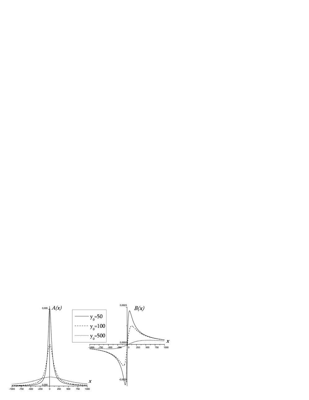
Figure 2: The real $A(x)$ and imaginary $B(x)$ parts of $\frac{1}{2\pi i}\,G^{(+)}_{0}\left(-\frac{2}{k};\;\mathcal{E}\right)$ for $\mathcal{E}=x+iy_{0}$ with different $y_{0}$.

with different $y_{0}$ are presented in Table 1. Note that the integrand in (28) involves hypergeometric functions ${{}_{2}F_{1}(a,\,b;\;a+b;\;z)}$. We found that the Gauss continued fraction Erdelyi (rather than the infinite sum (15.3.10) in Abramowitz ) provides an efficient approximation for the hypergeometric functions. The integrals are computed using IMSL FORTRAN Library routines. The real and imaginary parts of the integrand identified as $A(x)$ and $B(x)$ are displayed in Fig. 2 for different $y_{0}$. It is seen in Fig. 2 that $B(x)$ tends to zero as the parameter $y_{0}$ increases uniformly with respect to $x$. This property of $B(x)$ is consistent with the negligible imaginary parts of the integrals in Table 1. Using this observation, and (23), we conclude that

$$v^{(1)}_{0}=v^{(2)}_{0}=1=\frac{1}{2}\,v_{0}.$$ (29)

Moreover, our numerical computations show that

$$v^{(1)}_{n\,m;\;n^{\prime}\,m^{\prime}}=v^{(2)}_{n\,m;\;n^{\prime}\,m^{\prime}}=\frac{1}{2}\,v_{n\,m;\;n^{\prime}\,m^{\prime}}$$ (30)

holds for arbitrary $n,\,m,\,n^{\prime},\,m^{\prime}$.

Another straight-line path is obtained by rotating the contour $\mathcal{C}_{1}$ about some point $x_{0}$ on the positive real axis through an angle $\varphi$ in the range $-\pi<\varphi<0$ Shakeshaft ; JP2 . For definiteness, we choose $x_{0}=\frac{k}{2}$ and $\varphi=-\frac{\pi}{2}$, i. e. $\mathcal{E}=\frac{k}{2}+iy$ on the resulting contour $\mathcal{C}_{3}$, shown in Fig. 3. The path $\mathcal{C}_{3}$ crosses the cut so that its lower part (depicted in Fig. 3 by the dashed line) descends into the “unphysical” sheet ($-2\pi<\arg(\mathcal{E})<0$). To analytically continue matrix elements of ${\bf g}^{\xi(+)}$ and ${\bf g}^{\eta(+)}$ in (70) onto the unphysical sheet we use the formulae (66) and (67). Note that the numerical result for the integral

$$v^{(3)}_{0}=\frac{1}{2\pi}\,\int\limits_{\infty}^{-\infty}dy\,G^{(+)}_{0}\left(-\frac{2}{k};\;\frac{k^{2}}{2}+iy\right)$$ (31)

presented in Table 1 also satisfies

$$v^{(3)}_{0}=\frac{1}{2}\,v_{0}.$$ (32)

Thus, we find another straight-line path $\mathcal{C}_{3}$ for which

$$v^{(3)}_{n\,m;\;n^{\prime}\,m^{\prime}}=\frac{1}{2\pi i}\int\limits_{\mathcal{C}_{3}}d\mathcal{E}\,G^{(+)}_{n\,m;\;n^{\prime}\,m^{\prime}}\left(t;\;\mathcal{E}\right)=\frac{1}{2}\,v_{n\,m;\;n^{\prime}\,m^{\prime}}.$$ (33)

IV Double integrals

Now that we have the relationships (30) and (33) between the integrals along the contour $\mathcal{C}$ and the integrals over the straight-line paths, we can use $\mathcal{C}_{1}$ and $\mathcal{C}_{3}$ in the integral representation (19) of the Green’s function operator. Before proceeding, we consider the matrix product $\underline{\mathfrak{h}}\,\underline{\mathfrak{G}}^{(+)}$ to determine the normalizing factors $\aleph$ corresponding to the paths $\mathcal{C}_{1}$ and $\mathcal{C}_{3}$. Using the six-dimensional operator $\hat{\mathfrak{h}}$ (11) matrix representation

$$\underline{\mathfrak{h}}=\mu_{13}\mu_{12}{\bf h}_{1}\otimes{\bf Q}_{2}\otimes{\bf Q}_{3}+\mu_{23}\mu_{12}{\bf Q}_{1}\otimes{\bf h}_{2}\otimes{\bf Q}_{3}+\mu_{23}\mu_{13}{\bf Q}_{1}\otimes{\bf Q}_{2}\otimes{\bf h}_{3},$$ (34)

(19) and (20), we have

$$\underline{\mathfrak{h}}\,\underline{\mathfrak{G}}^{(+)}=\aleph\left\{{\bf W}_{1}+{\bf W}_{2}+{\bf W}_{3}\right\},$$ (35)

where

$$\begin{array}[]{c}{\bf W}_{1}=\frac{1}{(2\pi i)^{2}}\frac{\mu_{12}}{\mu_{23}}\int\limits_{\mathcal{C}^{(1)}}\int\limits_{\mathcal{C}^{(2)}}d\mathcal{E}_{1}d\mathcal{E}_{2}\;{\bf I}_{1}\otimes\left[{\bf Q}_{2}{\bf G}^{(+)}\left(t_{13};\;\mathcal{E}_{2}\right)\right]\\[8.53581pt] \otimes\left[{\bf Q}_{3}{\bf G}^{(+)}\left(t_{12};\;\frac{k_{12}^{2}}{2}+\frac{\mu_{12}}{\mu_{23}}\left(\frac{k_{23}^{2}}{2}-\mathcal{E}_{1}\right)+\frac{\mu_{12}}{\mu_{13}}\left(\frac{k_{13}^{2}}{2}-\mathcal{E}_{2}\right)\right)\right],\\ \end{array}$$ (36)

$$\begin{array}[]{c}{\bf W}_{2}=\frac{1}{(2\pi i)^{2}}\frac{\mu_{12}}{\mu_{13}}\int\limits_{\mathcal{C}^{(1)}}\int\limits_{\mathcal{C}^{(2)}}d\mathcal{E}_{1}d\mathcal{E}_{2}\;\left[{\bf Q}_{1}{\bf G}^{(+)}\left(t_{23};\;\mathcal{E}_{1}\right)\right]\otimes{\bf I}_{2}\\[8.53581pt] \otimes\left[{\bf Q}_{3}{\bf G}^{(+)}\left(t_{12};\;\frac{k_{12}^{2}}{2}+\frac{\mu_{12}}{\mu_{23}}\left(\frac{k_{23}^{2}}{2}-\mathcal{E}_{1}\right)+\frac{\mu_{12}}{\mu_{13}}\left(\frac{k_{13}^{2}}{2}-\mathcal{E}_{2}\right)\right)\right],\\ \end{array}$$ (37)

$${\bf W}_{3}=\frac{1}{(2\pi i)^{2}}\int\limits_{\mathcal{C}^{(1)}}\int\limits_{\mathcal{C}^{(2)}}d\mathcal{E}_{1}d\mathcal{E}_{2}\;\left[{\bf Q}_{1}{\bf G}^{(+)}\left(t_{23};\;\mathcal{E}_{1}\right)\right]\otimes\left[{\bf Q}_{2}{\bf G}^{(+)}\left(t_{13};\;\mathcal{E}_{2}\right)\right]\otimes{\bf I}_{3}.$$ (38)

The matrices $\underline{\mathfrak{h}}$ and $\underline{\mathfrak{G}}^{(+)}$ must be inverses of each other. Therefore, the normalizing factor $\aleph$ and the matrices ${\bf W}_{j}$, $j=\overline{1,\,3}$ satisfy the condition

$$\aleph\left\{{\bf W}_{1}+{\bf W}_{2}+{\bf W}_{3}\right\}={\bf I}.$$ (39)

If we choose $\mathcal{C}^{(1)}=\mathcal{C}_{1}$ and $\mathcal{C}^{(2)}=\mathcal{C}_{1}$ (or $\mathcal{C}^{(1)}=\mathcal{C}^{(2)}=\mathcal{C}_{3}$), then it follows from (22) and (30) (or (33)) that

$${\bf W}_{3}=\frac{1}{4}\,{\bf I}_{1}\otimes{\bf I}_{2}\otimes{\bf I}_{3}=\frac{1}{4}\,{\bf I}.$$ (40)

Further, we assume that

$${\bf W}_{1}=\frac{\alpha}{4}\,{\bf I},\quad{\bf W}_{2}=\frac{\beta}{4}\,{\bf I},$$ (41)

so that the sum $\left\{{\bf W}_{1}+{\bf W}_{2}+{\bf W}_{3}\right\}$ is proportional to the unit matrix ${\bf I}$. In turn, the constants $\alpha$ and $\beta$ can be determined by, e. g., the ratios

$$\alpha=\frac{w_{1}}{w_{3}},\qquad\beta=\frac{w_{2}}{w_{3}},$$ (42)

where

$$\begin{array}[]{c}w_{1}=\frac{1}{(2\pi i)^{2}}\frac{\mu_{12}}{\mu_{23}}\int\limits_{\mathcal{C}^{(1)}}\int\limits_{\mathcal{C}^{(2)}}d\mathcal{E}_{1}d\mathcal{E}_{2}\,G^{(+)}_{0}\left(t_{13};\;\mathcal{E}_{2}\right)\\[11.38109pt] \times G^{(+)}_{0}\left(t_{12};\;\frac{k_{12}^{2}}{2}+\frac{\mu_{12}}{\mu_{23}}\left(\frac{k_{23}^{2}}{2}-\mathcal{E}_{1}\right)+\frac{\mu_{12}}{\mu_{13}}\left(\frac{k_{13}^{2}}{2}-\mathcal{E}_{2}\right)\right),\\[11.38109pt] w_{2}=\frac{1}{(2\pi i)^{2}}\frac{\mu_{12}}{\mu_{13}}\int\limits_{\mathcal{C}^{(1)}}\int\limits_{\mathcal{C}^{(2)}}d\mathcal{E}_{1}d\mathcal{E}_{2}\,G^{(+)}_{0}\left(t_{23};\;\mathcal{E}_{1}\right)\\[11.38109pt] \times G^{(+)}_{0}\left(t_{12};\;\frac{k_{12}^{2}}{2}+\frac{\mu_{12}}{\mu_{23}}\left(\frac{k_{23}^{2}}{2}-\mathcal{E}_{1}\right)+\frac{\mu_{12}}{\mu_{13}}\left(\frac{k_{13}^{2}}{2}-\mathcal{E}_{2}\right)\right),\\[11.38109pt] w_{3}=\frac{1}{(2\pi i)^{2}}\int\limits_{\mathcal{C}^{(1)}}\int\limits_{\mathcal{C}^{(2)}}d\mathcal{E}_{1}d\mathcal{E}_{2}\,G^{(+)}_{0}\left(t_{23};\;\mathcal{E}_{1}\right)G^{(+)}_{0}\left(t_{13};\;\mathcal{E}_{2}\right).\\ \end{array}$$ (43)

Thereafter, the normalizing factor $\aleph$ is expressed as

$$\aleph=\frac{4}{1+\alpha+\beta}.$$ (44)

First we consider the path $\mathcal{C}_{1}$.

a) $\mathcal{C}^{(1)}=\mathcal{C}^{(2)}=\mathcal{C}_{1}$

In this case the energies $\mathcal{E}_{1}$ and $\mathcal{E}_{2}$ are parametrized by $\mathcal{E}_{1}=iy_{0}+x_{1}$ and $\mathcal{E}_{2}=iy_{0}+x_{2}$ with $y_{0}=100$. Assuming that the energy $\mathcal{E}_{3}=k^{2}-iy_{0}-\frac{1}{2}\left(x_{1}+x_{2}\right)$ lies on the “physical” sheet i. e. $0<\arg(\mathcal{E}_{3})<2\pi$, in view of (26)-(29), we obtain that

$$\begin{array}[]{c}\frac{1}{2\pi i}\int\limits_{-\infty}^{\infty}dx\,G^{(+)}_{0}\left(\frac{1}{2k};\;k^{2}-iy_{0}-\frac{1}{2}x\right)=2\frac{1}{2\pi i}\int\limits_{-\infty}^{\infty}dx\,G^{(+)}_{0}\left(\frac{1}{2k};\;k^{2}-iy_{0}+x\right)\\[11.38109pt] =-2\frac{1}{2\pi i}\int\limits_{\mathcal{C}_{2}}d\mathcal{E}\,G^{(+)}_{0}\left(\frac{1}{2k};\;\mathcal{E}\right)=-2v^{(2)}_{0}=-2v^{(1)}_{0}.\\ \end{array}$$ (45)

Hence, one might expect that the constants $\alpha$ and $\beta$ (42) are negative. Note that in our case the integrals $w_{j}$ (43) take the forms

$$\begin{array}[]{c}w_{1}=-\frac{1}{(2\pi)^{2}}\frac{1}{2}\mathop{\int\int}\limits_{-\infty}^{\infty}dx_{1}dx_{2}\,G^{(+)}_{0}\left(-\frac{2}{k};\;iy_{0}+x_{2}\right)\,G^{(+)}_{0}\left(\frac{1}{2k};\;k^{2}-iy_{0}-\frac{1}{2}\left(x_{1}+x_{2}\right)\right),\\[11.38109pt] w_{2}=-\frac{1}{(2\pi)^{2}}\frac{1}{2}\mathop{\int\int}\limits_{-\infty}^{\infty}dx_{1}dx_{2}\,G^{(+)}_{0}\left(-\frac{2}{k};\;iy_{0}+x_{1}\right)\,G^{(+)}_{0}\left(\frac{1}{2k};\;k^{2}-iy_{0}-\frac{1}{2}\left(x_{1}+x_{2}\right)\right),\\[11.38109pt] w_{3}=-\frac{1}{(2\pi)^{2}}\mathop{\int\int}\limits_{-\infty}^{\infty}dx_{1}dx_{2}\,G^{(+)}_{0}\left(-\frac{2}{k};\;iy_{0}+x_{1}\right)\,G^{(+)}_{0}\left(-\frac{2}{k};\;iy_{0}+x_{2}\right).\\ \end{array}$$ (46)

From the numerical results for the double integrals (46) presented in Table 1, it follows that $w_{1}=w_{2}=-\frac{1}{2}$ and $w_{3}=1$, i. e. $\alpha=\beta=-\frac{1}{2}$. Thus, we have $\alpha+\beta+1=0$, and so the equation (44) is meaningless. This outcome is consistent with the numerical result obtained for the integral in the expression (19) for the diagonal matrix element of $\left[\underline{\mathfrak{G}}^{(+)}\right]_{0,\,0}$ corresponding to the basis function $\left|0\right>\equiv\left|n_{j}=m_{j}=0,\,j=\overline{1,\,3}\right>$ (14):

$$\begin{array}[]{c}\mathcal{I}_{0}=\frac{1}{(2\pi i)^{2}}\mathop{\int\int}\limits_{-\infty}^{\infty}dx_{1}dx_{2}\,G^{(+)}_{0}\left(-\frac{2}{k};\;iy_{0}+x_{1}\right)\,G^{(+)}_{0}\left(-\frac{2}{k};\;iy_{0}+x_{2}\right)\\[11.38109pt] \times G_{0}\left(\frac{1}{2k};\;k^{2}-iy_{0}-\frac{1}{2}\left(x_{1}+x_{2}\right)\right),\\ \end{array}$$ (47)

which is presented in Table 1. Therefore, we conclude that the contour $\mathcal{C}_{1}$ cannot be used in the integral representation (19).

Now consider the the contour $\mathcal{C}_{3}$.

b) $\mathcal{C}^{(1)}=\mathcal{C}^{(2)}=\mathcal{C}_{3}$

The energies $\mathcal{E}_{1}$ and $\mathcal{E}_{2}$ are given by $\mathcal{E}_{1}=\frac{k^{2}}{2}+iy_{1}$ and $\mathcal{E}_{2}=\frac{k^{2}}{2}+iy_{2}$ on the contour $\mathcal{C}_{3}$. In turn, the energy $\mathcal{E}_{3}$ is parametrized as $\mathcal{E}_{3}=\frac{k^{2}}{2}-\frac{i}{2}\left(y_{1}+y_{2}\right)$. In this case the contour integrals (43) are transformed into the double integrals

$$\begin{array}[]{c}w_{1}=\frac{1}{(2\pi)^{2}}\frac{1}{2}\mathop{\int\int}\limits_{+\infty}^{-\infty}dy_{1}dy_{2}\,G^{(+)}_{0}\left(-\frac{2}{k};\;\frac{k^{2}}{2}+iy_{2}\right)\,G^{(+)}_{0}\left(\frac{1}{2k};\;\frac{k^{2}}{2}-\frac{i}{2}\left(y_{1}+y_{2}\right)\right),\\[11.38109pt] w_{2}=\frac{1}{(2\pi)^{2}}\frac{1}{2}\mathop{\int\int}\limits_{+\infty}^{-\infty}dy_{1}dy_{2}\,G^{(+)}_{0}\left(-\frac{2}{k};\;\frac{k^{2}}{2}+iy_{1}\right)\,G^{(+)}_{0}\left(\frac{1}{2k};\;\frac{k^{2}}{2}-\frac{i}{2}\left(y_{1}+y_{2}\right)\right),\\[11.38109pt] w_{3}=\frac{1}{(2\pi)^{2}}\mathop{\int\int}\limits_{+\infty}^{-\infty}dy_{1}dy_{2}\,G^{(+)}_{0}\left(-\frac{2}{k};\;\frac{k^{2}}{2}+iy_{1}\right)\,G^{(+)}_{0}\left(-\frac{2}{k};\;\frac{k^{2}}{2}+iy_{2}\right).\\ \end{array}$$ (48)

Notice that from (31) it follows that

$$\frac{1}{2\pi}\,\int\limits_{+\infty}^{-\infty}dy\,G^{(+)}_{0}\left(\frac{1}{2k};\;\frac{k^{2}}{2}-\frac{i}{2}y\right)=2\left[\frac{1}{2\pi}\,\int\limits_{+\infty}^{-\infty}dy\,G^{(+)}_{0}\left(\frac{1}{2k};\;\frac{k^{2}}{2}+iy\right)\right]=2v^{(3)}_{0}.$$ (49)

Therefore, in contrast to the previous case, $w_{1}$ ($w_{2}$) would be expected to have the same sign as $w_{3}$. From the result for the numerical evaluations of the integrals (48), presented in Table 1., it follows that $w_{1}=w_{2}=\frac{3}{2}$ and $w_{3}=1$. Hence $\alpha=\beta=\frac{3}{2}$ and $\aleph=1$.

To verify that the straight-line path $\mathcal{C}_{3}$ does provide the desired result, we evaluate numerically the matrix elements

$$\begin{array}[]{c}\left[\underline{\mathfrak{G}}^{(+)}\right]_{\mathfrak{N},\,\mathfrak{N}^{\prime}}=\frac{1}{(2\pi)^{2}}\mathop{\int\int}\limits_{+\infty}^{-\infty}dy_{1}dy_{2}\,G^{(+)}_{n_{1}\,m_{1};\;n_{1}^{\prime}\,m_{1}^{\prime}}\left(-\frac{2}{k};\;\frac{k^{2}}{2}+iy_{1}\right)\\[11.38109pt] \times G^{(+)}_{n_{2}\,m_{2};\;n_{2}^{\prime}\,m_{2}^{\prime}}\left(-\frac{2}{k};\;\frac{k^{2}}{2}+iy_{2}\right)\,G^{(+)}_{n_{3}\,m_{3};\;n_{3}^{\prime}\,m_{3}^{\prime}}\left(\frac{1}{2k};\;\frac{k^{2}}{2}-\frac{i}{2}\left(y_{1}+y_{2}\right)\right)\\ \end{array}$$ (50)

and calculate the matrix product $\underline{\mathfrak{h}}\,\underline{\mathfrak{G}}^{(+)}$ of finite size. Notice that the matrix $\underline{\mathfrak{h}}$ (34) is “tridiagonal”, i. e. for each pair of indices $\left\{n_{j},\,n_{j}^{\prime}\right\}$ and $\left\{m_{j},\,m_{j}^{\prime}\right\}$, $j=\overline{1,\,3}$, the elements $\left[\underline{\mathfrak{h}}\right]_{\mathfrak{N},\,\mathfrak{N}^{\prime}}$ vanish unless $\left|n_{j}-n_{j}^{\prime}\right|\leq 1$ and $\left|m_{j}-m_{j}^{\prime}\right|\leq 1$. Therefore, the minimal rank $\mathcal{N}_{min}$ of the matrices $\underline{\mathfrak{h}}$ and $\underline{\mathfrak{G}}$, with which the relation $\underline{\mathfrak{h}}\underline{\mathfrak{G}}={\bf I}$ could be verified, is given by $\mathcal{N}_{min}=2^{6}=64$. Actually, to test this equality, we must use all the basis functions $\left|\mathfrak{N}\right>$ (14) with each of the $n_{j}$ and $m_{j}$ taking the value one or zero. Our prime interest here is with the values of the first row elements $\left[\underline{\mathfrak{h}}\underline{\mathfrak{G}}^{(+)}\right]_{0,\,\mathfrak{N}}$ in the matrix $\underline{\mathfrak{h}}\underline{\mathfrak{G}}^{(+)}$. The numerical result for the first diagonal element $\left[\underline{\mathfrak{h}}\underline{\mathfrak{G}}^{(+)}\right]_{0,\,0}$, presented in Table 1, corresponds to the inverse relationship between $\underline{\mathfrak{h}}$ and $\underline{\mathfrak{G}}$. In turn, the remaining (zero) elements of the first row are found to be of the order of $10^{-7}$.

V Conclusion

In this paper we focus attention on the three-body Coulomb Green’s function operator representation. The development of our method is based primarily upon the fact that for large particle separation the Schrödinger equation is separable in terms of generalized parabolic coordinates. Thus, the corresponding six-dimensional resolvent operator can be expressed as a convolution of three two-dimensional Greens function. This representation includes integration along contours, which encircle the spectra of two-dimensional wave operators. Unfortunately, these (double) contour integrals are very inconvenient for numerical computation. Clearly, it is preferable to employ straight-lane paths of integration. In this paper we demonstrate numerically, with two simple examples, that use of an appropriate straight-line path of integration provides a non-zero integral representation of the Green’s function operator.

Appendix A Matrix representations of one- and two-dimensional operators

A.1 One-dimensional operators

The matrix representation ${\bf h}_{\xi}$ of the operator $\hat{\mathfrak{h}}_{\xi}$ (9) in the basis $\left\{\psi_{n}(\xi)\right\}_{n=0}^{\infty}$ (16), which is orthonormal with respect $\xi\in[0,\,\infty)$, is tridiagonal with nonzero elements

$$h^{\xi}_{n,\,n}=b+ik+2bn,\quad h^{\xi}_{n,\,n-1}=(b-ik)n,\quad h^{\xi}_{n,\,n+1}=(b+ik)(n+1).$$ (51)

In addition, the symmetric matrix ${\bf Q}_{\xi}$ of the operator $\xi$ in the basis (16) is also tridiagonal:

$$Q_{n,\,n^{\prime}}=\left\{\begin{array}[]{lr}-\frac{n}{2b},&n^{\prime}=n-1,\\ \frac{2n+1}{2b},&n^{\prime}=n,\\ -\frac{n+1}{2b},&n^{\prime}=n+1.\\ \end{array}\right.$$ (52)

Hence, the one-dimensional operator $\left[\hat{\mathfrak{h}}_{\xi}+2kt+\mu C\xi\right]$ also has the tridiagonal matrix representation $\left[{\bf h}_{\xi}+2kt{\bf I}_{\xi}+\mu C{\bf Q}_{\xi}\right]$ (${\bf I}_{\xi}$ is the unit matrix) in the basis set (16). Fortunately, the inverse of the matrix $\left[{\bf h}_{\xi}+2kt{\bf I}_{\xi}+\mu C{\bf Q}_{\xi}\right]$ can be obtained analytically. The elements of the resulting matrix ${\bf g}^{\xi(\pm)}$ are expressed in terms of well-known special functions

$$g^{\xi(+)}_{n_{1},\,n_{2}}(\tau;\;\gamma) = \frac{i}{2\gamma}\left(\frac{\zeta-1}{\zeta}\right)\frac{\theta^{n_{1}-n_{2}}}{\zeta^{n_{2}}}\,p_{n_{<}}(\tau;\;\zeta)\,q_{n_{>}}^{(+)}(\tau;\;\zeta),$$ (53)

$$g^{\xi(-)}_{n_{1},\,n_{2}}(\tau;\;\gamma) = \frac{i}{2\gamma}\left(\frac{\zeta-1}{\zeta}\right)\frac{\theta^{n_{1}-n_{2}}}{\zeta^{n_{2}}}\,p_{n_{<}}(\tau;\;\zeta)\,\zeta^{n_{>}+1}\,q_{n_{>}}^{(-)}(\tau;\;\zeta),$$ (54)

where $n_{<}$ is the lesser of $n_{1}$ and $n_{2}$, and $n_{>}$ the greater of the two. Here

$$\theta=\frac{2b+i(\gamma-k)}{2b-i(\gamma-k)},\quad\lambda=\frac{2b-i(\gamma+k)}{2b+i(\gamma+k)},\quad\zeta=\frac{\lambda}{\theta},$$ (55)

$$\tau=\frac{k}{\gamma}\left(t+\frac{i}{2}\right),$$ (56)

$$\mu C=\frac{k^{2}}{2}-\mathcal{E},\quad\mathcal{E}=\frac{\gamma^{2}}{2},$$ (57)

and

$$p_{n}(\tau;\;\zeta)=\frac{(-1)^{n}}{n!}\frac{\Gamma\left(n+\frac{1}{2}-i\tau\right)}{\Gamma\left(\frac{1}{2}-i\tau\right)}\;{{}_{2}F_{1}\left(-n,\,\frac{1}{2}+i\tau;\;-n+\frac{1}{2}+i\tau;\;\zeta\right)}$$ (58)

are the polynomials of degree $n$ in $\tau$ which are orthogonal,

$$\frac{i}{\zeta^{m}}\left(\frac{\zeta-1}{\zeta}\right)\int\limits_{-\infty}^{\infty}d\tau\,\rho(\tau;\;\zeta)p_{n}(\tau;\;\zeta)p_{m}(\tau;\;\zeta)=\delta_{n\,m},$$ (59)

with respect to the weight function,

$$\rho(\tau;\;\zeta)=\frac{1}{2\pi i}\Gamma\left(\frac{1}{2}+i\tau\right)\Gamma\left(\frac{1}{2}-i\tau\right)(-\zeta)^{i\tau+\frac{1}{2}}.$$ (60)

In (60) it is considered that $|\arg(-\zeta)|<\pi$. The function $q_{n}^{(\pm)}$ is given by

$$q_{n}^{(\pm)}(\tau;\;\zeta)=(-1)^{n}\frac{n!\Gamma\left(\frac{1}{2}\pm i\tau\right)}{\Gamma\left(n+\frac{3}{2}\pm i\tau\right)}\;{{}_{2}F_{1}\left(\frac{1}{2}\pm i\tau,\,n+1;\;n+\frac{3}{2}\pm i\tau;\;\zeta^{\mp 1}\right)}.$$ (61)

Similarly, the nonzero elements of the tridiagonal matrix ${\bf h}_{\eta}$ of the operator $\hat{\mathfrak{h}}_{\eta}$ (9) in the basis $\left\{\psi_{n}(\eta)\right\}_{n=0}^{\infty}$ (16) are

$$h^{\eta}_{n,\,n}=b-ik+2bn,\quad h^{\eta}_{n,\,n-1}=(b+ik)n,\quad h^{\eta}_{n,\,n+1}=(b-ik)(n+1).$$ (62)

Obviously, the nonzero elements of the matrix ${\bf Q}_{\eta}$ of the operator $\eta$ in the basis (16) are defined by (52). Thus, the elements of the matrix ${\bf g}^{\eta(\pm)}$, which is inverse of the matrix $\left[{\bf h}_{\eta}+2kt{\bf I}_{\eta}+\mu C{\bf Q}_{\eta}\right]$ (${\bf I}_{\eta}$ is the unit matrix) of the one-dimensional operator $\left[\hat{\mathfrak{h}}_{\eta}+2kt+\mu C\eta\right]$, are expressed as

$$g^{\eta(+)}_{n_{1},\,n_{2}}(\tau;\;\gamma) = \frac{i}{2\gamma}\left(\frac{\zeta-1}{\zeta}\right)\frac{\lambda^{n_{2}-n_{1}}}{\zeta^{n_{2}}}\,p_{n_{<}}(\tau;\;\zeta)\,q_{n_{>}}^{(+)}(\tau;\;\zeta),$$ (63)

$$g^{\eta(-)}_{n_{1},\,n_{2}}(\tau;\;\gamma) = \frac{i}{2\gamma}\left(\frac{\zeta-1}{\zeta}\right)\frac{\lambda^{n_{2}-n_{1}}}{\zeta^{n_{2}}}\,p_{n_{<}}(\tau;\;\zeta)\,\zeta^{n_{>}+1}\,q_{n_{>}}^{(-)}(\tau;\;\zeta).$$ (64)

Note that $q_{n}^{(+)}$ $\left(q_{n}^{(-)}\right)$ are defined in the upper (lower) half of the complex $\gamma$ plane where $|\zeta|>1$ ($|\zeta|<1$). $q_{n}^{(+)}$ can be analytically continued onto the lower half-plane by using the relation for hypergeometric functions (15.3.7) in Abramowitz , which transforms into the following relationship between $q_{n}^{(+)}$ and $q_{n}^{(-)}$:

$$q_{n}^{(+)}(\tau;\;\zeta)=\zeta^{n+1}q_{n}^{(-)}(\tau;\;\zeta)+2\pi i\rho(\tau;\;\zeta)p_{n}(\tau;\;\zeta)$$ (65)

Then the formulae for the analytical continuations of $g^{\xi(+)}_{n_{1},\,n_{2}}$ and $g^{\eta(+)}_{n_{1},\,n_{2}}$ are

$$g^{\xi(+)}_{n_{1},\,n_{2}}(\tau;\;\gamma) = g^{\xi(-)}_{n_{1},\,n_{2}}(\tau;\;\gamma)-\frac{\pi}{\gamma}\left(\frac{\zeta-1}{\zeta}\right)\frac{\theta^{n_{1}}}{\lambda^{n_{2}}}\,\rho(\tau;\;\zeta)\,p_{n_{1}}(\tau;\;\zeta)\,p_{n_{2}}(\tau;\;\zeta),$$ (66)

$$g^{\eta(+)}_{n_{1},\,n_{2}}(\tau;\;\gamma) = g^{\eta(-)}_{n_{1},\,n_{2}}(\tau;\;\gamma)-\frac{\pi}{\gamma}\left(\frac{\zeta-1}{\zeta}\right)\frac{\theta^{n_{2}}}{\lambda^{n_{1}}}\rho(\tau;\;\zeta)\,p_{n_{1}}(\tau;\;\zeta)\,p_{n_{2}}(\tau;\;\zeta).$$ (67)

A.2 Two-dimensional operators

Note first that the completeness relations for eigenfunctions of the one-dimensional operators $\left[\hat{\mathfrak{h}}_{\xi}+2kt+\mu C\xi\right]$ and $\left[\hat{\mathfrak{h}}_{\eta}+2kt+\mu C\eta\right]$ may take the form (see, e. g., JP1 )

$$\pm\frac{\gamma}{i\pi}\int\limits_{-\infty}^{\infty}d\tau\,g_{n_{1},\,n_{2}}^{\xi(\pm)}(\tau;\;\zeta)=\pm\frac{\gamma}{i\pi}\int\limits_{-\infty}^{\infty}d\tau\,g_{n_{1},\,n_{2}}^{\eta(\pm)}(\tau;\;\zeta)=\frac{1}{2}\,\delta_{n_{1},\,n_{2}}.$$ (68)

The two-dimensional operator $\left[\hat{\mathfrak{h}}_{\xi}+\hat{\mathfrak{h}}_{\eta}+2kt_{0}+\mu C(\xi+\eta)\right]$ is also treated analytically within the context of the basis $\left\{\phi_{n,\,m}(\xi,\,\eta)\right\}_{n,\,m=0}^{\infty}$ (15). In particular, in view of (68), the inverse of the infinite matrix

$$\left[{\bf h}_{\xi}\otimes{\bf I}_{\eta}+{\bf I}_{\xi}\otimes{\bf h}_{\eta}+2kt_{0}{\bf I}_{\xi}\otimes{\bf I}_{\eta}+\mu C\left({\bf Q}_{\xi}\otimes{\bf I}_{\eta}+{\bf I}_{\xi}\otimes{\bf Q}_{\eta}\right)\right]$$ (69)

can be represented in the form of a convolution integral

$${\bf G}^{(\pm)}(t_{0};\;\mathcal{E})=\pm\frac{\gamma}{i\pi}\int\limits_{-\infty}^{\infty}d\tau\,{\bf g}^{\xi(\pm)}(\tau;\;\gamma)\otimes{\bf g}^{\eta(\pm)}(\tau_{0}-\tau;\;\gamma)$$ (70)

where $\tau_{0}=\frac{k}{\gamma}\,t_{0}$. Finally we noted that the matrix representation ${\bf G}^{(\pm)}$ (70) of the two-dimensional Green’s function operator is symmetric in $\xi$ and $\eta$ unlike the corresponding formula obtained in JP2 .

Figure 1: The paths of integration on the physical energy sheet. The gray line is the branch cut along the positive real axis. The poles of the integrand in (22) which occur at $\mathcal{E}_{\ell}=-\frac{\left(kt\right)^{2}}{2\ell^{2}}$, $\ell=1,2,\,\ldots$ for $t<0$ are shown as solid circles.

Figure 3: The path of integration $\mathcal{C}_{3}$. The solid line is the part of $\mathcal{C}_{3}$ which remains on the physical sheet. The part of $\mathcal{C}_{3}$ which moves onto the unphysical sheet is depicted by the dashed line.

Table 1: The numerical results obtained for integrals along the contours $\mathcal{C}_{1}$ and $\mathcal{C}_{3}$ and for the element $\left[\underline{\mathfrak{h}}\,\underline{\mathfrak{G}}^{(+)}\right]_{0,\,0}$ of the matrix product $\underline{\mathfrak{h}}\underline{\mathfrak{G}}^{(+)}$.

contour $\mathcal{C}_{1}$	contour $\mathcal{C}_{3}$
$\mathcal{E}_{1}=iy_{0}+x_{1}$, $\mathcal{E}_{1}=iy_{0}+x_{1}$,	$\mathcal{E}_{1}=\frac{k^{2}}{2}+iy_{1}$, $\mathcal{E}_{2}=\frac{k^{2}}{2}+iy_{2}$,
$\mathcal{E}_{3}=k^{2}-iy_{0}-\frac{1}{2}\left(x_{1}+x_{2}\right)$	$\mathcal{E}_{3}=\frac{k^{2}}{2}-\frac{i}{2}\left(y_{1}+y_{2}\right)$
$y_{0}=50\hphantom{0}$, $v^{(1)}_{0}=0.99996555-i\,2.7568672\times 10^{-6}$	$v^{(3)}_{0}=1.0000132-i\,1.0613277\times 10^{-4}$
$y_{0}=100$, $v^{(1)}_{0}=0.99996555+i\,4.8873452\times 10^{-6}$
$y_{0}=500$, $v^{(1)}_{0}=0.99996539+i\,4.9623285\times 10^{-6}$
$y_{0}=100$
$\begin{array}[]{l}w_{1}=-0.50009660-i\,0.75786560\times 10^{-4}\\ w_{2}=-0.50011010-i\,0.77244545\times 10^{-4}\\ w_{3}=\hphantom{-}1.00013285-i\,1.3211843\times 10^{-4}\\ \mathcal{I}_{0}=0.79996314\times 10^{-9}-i\,0.62352239\times 10^{-8}\\ \end{array}$	$\begin{array}[]{l}w_{1}=1.49998186-i\,0.36607003\times 10^{-3}\\ w_{2}=1.49996754-i\,0.36818990\times 10^{-3}\\ w_{3}=0.99998324-i\,0.42641600\times 10^{-3}\\ \left[\underline{\mathfrak{h}}\underline{\mathfrak{G}}^{(+)}\right]_{0,\,0}=0.99999770-i\,2.3034284\times 10^{-5}\end{array}$

References

• (1) S. A. Zaytsev, J. Phys. A, 41 265204 (2008).
• (2) S. A. Zaytsev, J. Phys. A, 42 015202 (2009).
• (3) H. Klar, Z. Phys. D 16, 231 (1990).
• (4) Dz. Belkic, J. Phys. B 11, 3529 (1978).
• (5) C. R. Garibotti, J. E. Miraglia, Phys. Rev. A 21, 572 (1980).
• (6) M. Brauner, J. S. Briggs, H. Klar, J. Phys. B 22, 2265 (1989).
• (7) L. U. Ancarani and G. Gasaneo, Phys. Rev. A 75 032706 (2007).
• (8) P. C. Ojha, J. Math. Phys. 28, 392 (1987).
• (9) L. D. Faddeev and S. P. Merkuriev, Quantum Scattering Theory for Several Particle Systems (Kluwer Academic Publishers, Dordrecht, 1993).
• (10) Higher Transcendental Functions, edited by A. Erdelyi (McGraw-Hill, New York, 1953).
• (11) M. Abramowitz and I. A. Stegun, Handbook of mathematical functions (New York: Dover), 1970.
• (12) R. Shakeshaft, Phys. Rev. A, 70, 042704 (2004).
Refer to caption