Quilted Gabor frames - a new concept for adaptive time-frequency representation

Abstract.

Certain signal classes such as audio signals call for signal representations with the ability to adapt to the signal’s properties. In this article we introduce the new concept of quilted frames, which aim at adaptivity in time-frequency representations. As opposed to Gabor or wavelet frames, this new class of frames allows for the adaptation of the signal analysis to the local requirements of signals under consideration. Quilted frames are constructed directly in the time-frequency domain in a signal-adaptive manner. Validity of the frame property guarantees the possibility to reconstruct the original signal. The frame property is shown for specific situations and the Bessel property is proved for the general setting. Strategies for reconstruction from coefficients obtained with quilted Gabor frames and numerical simulations are provided as well.

1. Introduction

QUILT (verb): (a) to fill, pad, or line like a quilt
(b) to stitch (designs) through layers of cloth
(c) to fasten between two pieces of material

Natural signals usually comprise components of various different characteristics and their analysis requires judicious choice of processing tools. For audio signals time-frequency dictionaries have proved to be an adequate option. Since orthonormal bases cannot provide good time-frequency resolution, [22], time-frequency analysis naturally leads to the use of frames. Most classes of frames commonly used in applications, be it wavelet or Gabor frames, feature a resolution following a fixed rule over the whole time-frequency or time-scale plane, respectively. The concept of quilted frames, as introduced in this contribution, gives up this uniformity and allows for different resolutions in assigned areas of the time-frequency plane.
The primary motivation for introducing this new class of frames stems from the processing of audio and in particular music signals, where the trade-off between time- and frequency resolution has a strong impact on the results of analysis and synthesis, see [27, 10, 30, 28, 24]. The well-known uncertainty principle makes the choice of just one analysis window a difficult task: different resolutions might be favorable in order to achieve sparse and precise representations for the various signal components. For example, percussive elements require short analysis windows and high sampling rate in time, whereas sustained sinusoidal components are better represented with wide windows and a longer FFT, thus more sampling points in frequency.

Several approaches have been suggested to deal with the trade-off in time-frequency resolution. The notion of multi-window Gabor expansions, introduced by Zibulski and Zeevi, [31], uses a finite number of windows of different shape in order to obtain a richer dictionary with the ability to better represent certain characteristics in a given signal class. Another approach is the usage of several bases in order to best describe the components of a signal with a priori known characteristics, see [9]. All these approaches, however, stick to a uniform resolution guided by the action of a certain group via a unitary representation. For quilted Gabor frames we give up this restriction and introduce systems constructed from globally defined frames by restricting these to certain, possibly compact, regions in the time-frequency or time-scale plane. The idea of realizing tilings of the time-frequency plane has been suggested in [4] and [29], however, these authors stick to the construction of orthogonal bases. In this case, every basis function corresponds to a particular tile. We will achieve a wider range of possible partitions, windows and sampling schemes by allowing for redundancy. Thus we aim at designing systems that can optimally adapt to a class of signals considered. As a particular example of quilted frames, the notion of reduced multi-Gabor frames was first introduced in [11] and recently exploited in [24]. Note that this model allows, for example, a transform yielding constant-Q spectral resolution, which is invertible, as opposed to the original construction [5]. Reduced multi-Gabor frames were successfully applied to the task of denoising corrupted audio signals, see [30]. The processing of sound signals also yields a motivation for the next step in generalizing the idea to quilted frames, which allow arbitrary tilings of the time-frequency plane, see [25].
Quilted frames also bear theoretical interested in themselves and should be compared to constructions such as fusion frames [7] and the frames proposed in [1]. In fact, the construction of quilted frames provides constructive examples for the models presented in these contributions.
For the mathematical description of quilted frames, we start from principles of Gabor analysis [20]. The idea for the construction of quilted Gabor frames is inspired by the early work of Feichtinger and Gröbner on decomposition methods [18, 16] and recent results on time-frequency partitions for the characterization of function spaces [12, 13]:
Assume that a covering $(\Omega_{r})_{r\in\mathcal{I}}$ of the phase space $\mathbb{R}^{2d}$ is given. To each member of the covering a frame from a family of Gabor frames is assigned, hence, the new system locally resembles the original frames. The resulting global system will be called a quilted Gabor system. We conjecture that these systems may be shown to constitute frames under certain, rather general conditions. In this paper we will show the frame property in two special cases and proof the existence of an upper frame bound for a general setting.

The rest of this paper is organized as follows. Section 2 provides notation and gives an overview over basic results in Gabor analysis. Section 3 introduces the general concept of quilted Gabor frames. In Section 4, the existence of an upper frame bound (Bessel property) for general quilted frames is proved. In Section 5 and Section 6, a lower frame bound is constructed for two particular cases, namely, the partition of the time-frequency plane in stripes and the replacement of frame elements in a compact region of the coefficient domain. Finally, Section 7 presents numerical examples for these cases.

2. Notation and some basic facts from Gabor theory

We use the normalization $\hat{f}(\omega)=\int_{\mathbb{R}^{d}}f(t)e^{-2\pi i\omega t}dt$ of the Fourier transform on $\mathbf{L}^{2}(\mathbb{R}^{d})$. $M_{\omega}$ and $T_{x}$ denote frequency-shift by $\omega$ and time-shift by $x$, respectively, of a function $g$, combined to the time-frequency shift operators $\pi(\lambda)=M_{\omega}T_{x}g(t)=e^{2\pi it\omega}g(t-x)$ for $\lambda=(x,\omega)\in\mathbb{R}^{2d}$.

The Short-time Fourier transform (STFT) of a function $f\in\mathbf{L}^{2}(\mathbb{R}^{d})$ with respect to a window function $g\in\mathbf{L}^{2}(\mathbb{R}^{d})$ is defined as

(1) $$\mathcal{V}_{g}f(\lambda)=\int_{\mathbb{R}^{d}}f(t)\bar{g}(t-x)e^{-2\pi i\omega\cdot t}\,dt=\langle f,\pi(\lambda)g\rangle\,.$$

A lattice $\Lambda\subset\mathbb{R}^{2d}$ is a discrete subgroup of $\mathbb{R}^{2d}$ of the form $\Lambda=A\mathbb{Z}^{2d}$, where $A$ is an invertible $2d\times 2d$-matrix over $\mathbb{R}$. The special case $\Lambda=\alpha\mathbb{Z}^{d}\times\beta\mathbb{Z}^{d},$ where $\alpha,\beta>0$ are the lattice constants, is called a separable or product lattice.

A family of functions $(g_{k})_{k\in\mathbb{Z}}$ in $(\mathbb{R}^{d})$ is called a frame, if there exist lower and upper frame bounds $A,B>0$, so that

(2) $$A\|f\|^{2}\leq\sum_{k\in\mathbb{Z}}|\langle f,g_{k}\rangle|^{2}\leq B\|f\|^{2}\ \mbox{ for all }f\in\mathbf{L}^{2}(\mathbb{R}^{d})$$

Assumption (2) can be understood as an “approximate Plancherel formula”. It guarantees that any signal $f\in\mathbf{L}^{2}(\mathbb{R}^{d})$ can be represented as infinite series with square integrable coefficients using the elements $g_{k}$. The existence of the upper bound $B$ is called Bessel property of the sequence $(g_{k})_{k\in\mathbb{Z}}$. The frame operator $S$, defined as

$$Sf=\sum_{k\in\mathbb{Z}}\langle f,g_{k}\rangle g_{k}$$

allows the calculation of the canonical dual frame $(\gamma_{k})_{k\in\mathbb{Z}}=(S^{-1}g_{k})_{k\in\mathbb{Z}}$, which guarantees minimal-norm coefficients in the expansion

(3) $$f=\sum_{k\in\mathbb{Z}}\langle f,\gamma_{k}\rangle g_{k}=\sum_{k\in\mathbb{Z}}\langle f,g_{k}\rangle\gamma_{k}.$$

If $A=B$, the frame is called tight and $f=\frac{1}{A}\sum_{k}\langle f,g_{k}\rangle g_{k}$. We refer the interested reader to Christensen’s book [8] for more details on general frames.
In the special case of Gabor or Weyl-Heisenberg frames, the frame elements are generated by time-frequency shifts of a basic atom or window $g$ along a lattice $\Lambda$:

$$g_{\lambda}=\pi(\lambda)g.$$

In this case we write $S=S_{g}$, and $S_{g}=T_{g}^{\ast}T_{g}$, where $T_{g}:f\mapsto[\langle f,g_{\lambda}\rangle]_{\lambda}$ is the analysis operator mapping the function $f\in\mathbf{L}^{2}(\mathbb{R}^{d})$ to its coefficients $c(f)(\lambda)=T_{g}f(\lambda)$. These coefficients correspond to the samples of the STFT on $\Lambda$. Its adjoint $T_{g}^{\ast}:[c_{\lambda}]_{\lambda\in\Lambda}\mapsto\sum_{\lambda\in\Lambda}c_{\lambda}\pi(\lambda)g$ is the synthesis operator. For the Gabor frame generated by time-frequency shifts of the window $g$ along the lattice $\Lambda$ we write $\mathcal{G}(g,\Lambda)$.

We next introduce the concept of partitions of unity . A family $(\psi_{r})_{r\in\mathcal{I}}$ of non-negative functions with $\sum_{r}\psi_{r}(x)\equiv 1$ is called bounded admissible partition of unity (BAPU) subordinate to $(B_{R_{r}}(x_{r}))_{r\in\mathcal{I}}$, if the support $\Omega_{r}$ of $(\psi_{r})$ is contained in $B_{R_{r}}(x_{r})$ for $r\in\mathcal{I}$, and $(B_{R_{r}}(x_{r}))_{r\in\mathcal{I}}$ is an admissible covering in the sense of [14] i.e., $\bigcup_{r\in\mathcal{I}}B_{R_{r}}=\mathbb{R}^{d}$ and the number of overlapping $B_{R_{r}}(x_{r})$ is bounded above (admissibility condition). In other words, with

$$r^{\ast}:=\{s:s\in\mathcal{I},B_{R_{r}}(x_{r})\cap B_{R_{s}}(x_{s})\neq 0\},$$

for all $r\in\mathcal{I}$ there exists $n_{0}\in\mathbb{N}$, called height of the BAPU, such that $|r^{\ast}|\leq n_{0}$.

For technical reasons, which do not eliminate any interesting example, we assume even more: for all $\rho<\infty$ the family $(B_{R_{r}+\rho}(x_{r}))_{r\in\mathcal{I}}$ should be an admissible covering of $\mathbb{R}^{d}$. More precisely, we assume throughout this paper that for each $\rho>0$ there exists $n_{0}=n_{0}(\rho)\in\mathbb{N}$ such that the number of overlapping balls constituting the covering is uniformly controlled: $|r^{\ast}|\leq n_{0}$ for all $r\in\mathcal{I}$, where

$$r^{\ast}:=\{s:s\in\mathcal{I},B_{R_{r}+\rho}(x_{r})\cap B_{R_{s}}(x_{s}+\rho)\neq 0\}.$$

Obviously such coverings are of uniform height.
Using the concept of BAPUs, we now turn to Wiener amalgam spaces, introduced by H. Feichtinger in 1980 (see [17] for an accessible publication). The definition of Wiener amalgam spaces aims at decoupling local and global properties of $\mathbf{L}^{p}$-spaces. Let a BAPU $(\psi_{r})_{r\in\mathcal{I}}$ for $\mathbb{R}^{d}$ be given. The Wiener amalgam space ${\boldsymbol{W}}(\mathbf{L}^{p},\ell^{q})$ is defined as follows:

$${\boldsymbol{W}}(\mathbf{L}^{p},\ell^{q})(\mathbb{R}^{d})=\big{\{}f\in L^{p}_{loc}:\|f\|_{{\boldsymbol{W}}(\mathbf{L}^{p},\ell^{q})}=\big{(}\sum_{r\in\mathcal{I}}\|f\cdot\psi_{r}\|_{p}^{q}\big{)}^{\frac{1}{q}}<\infty\big{\}}.$$

We will denote by ${\boldsymbol{W}}(C^{0},\ell^{p})(\mathbb{R}^{d})\subseteq{\boldsymbol{W}}(\mathbf{L}^{\infty},\ell^{p})(\mathbb{R}^{d})$ the subspace of continuous, locally bounded functions in ${\boldsymbol{W}}(\mathbf{L}^{\infty},\ell^{p})(\mathbb{R}^{d})$. A comprehensive review of (weighted) Wiener amalgam spaces can be found in [23]. We note that in their most general form they are described as ${\boldsymbol{W}}(B,C)$, with local component $B$ and global component $C$. Let us recall some properties which will be needed later on:

• If $B_{1}\subseteq B_{2}$, $C_{1}\subseteq C_{2}$, then ${\boldsymbol{W}}(B_{1},C_{1})\subseteq{\boldsymbol{W}}(B_{2},C_{2})$.

• If $B_{1}\ast B_{2}\subseteq B_{3}$, $C_{1}\ast C_{2}\subseteq C_{3}$, then ${\boldsymbol{W}}(B_{1},C_{1})\ast{\boldsymbol{W}}(B_{2},C_{2})\subseteq{\boldsymbol{W}}(B_{3},C_{3})$.

A particularly important Banach space in time-frequency analysis is the Wiener Amalgam space ${\boldsymbol{W}}(\mathcal{F}L^{1},\ell^{1})$. This space, also known under the name Feichtinger’s algebra, is better known as the modulation space $M^{1,1}_{m}$, with constant weight $m\equiv 1$. It is often denoted by $S_{0}$ in the literature and we will adopt this name in the present work. For convenience, we also recall the definition of $S_{0}$ via the short-time Fourier transform.

Definition 1 ($S_{0}$).

Let $g_{0}$ be the Gauss-function $g_{0}=e^{-\pi\|x\|^{2}}$. The space $S_{0}(\mathbb{R}^{d})$ is given by

$$S_{0}(\mathbb{R}^{d})=\{f\in\mathbf{L}^{2}(\mathbb{R}^{d}):\|f\|_{S_{0}}=\|\mathcal{V}_{g_{0}}f\|_{\mathbf{L}^{1}(\mathbb{R}^{2d})}<\infty\}.$$

An in-depth investigation of $S_{0}(\mathbb{R}^{d})$ and its outstanding role in time-frequency analysis can be found in [15]. Note that $S_{0}(\mathbb{R}^{d})$ is densely embedded in $\mathbf{L}^{2}(\mathbb{R}^{d})$, with $\|f\|_{2}\leq\|g_{0}\|_{2}^{-1}\|f\|_{S_{0}}$. Its dual space $S_{0}^{\prime}(\mathbb{R}^{d})$, the space of all linear, continuous functionals on $S_{0}(\mathbb{R}^{d})$, contains $\mathbf{L}^{2}(\mathbb{R}^{d})$ and is a very convenient space of (tempered) distributions. Moreover, in the definition of $S_{0}(\mathbb{R}^{d})$, $g_{0}$ can be replaced by any $g\in S_{0}(\mathbb{R}^{d})$, see [22, Theorem 11.3.7] and different functions $g\in S_{0}(\mathbb{R}^{d})\setminus\{0\}$ define equivalent norms on $S_{0}(\mathbb{R}^{d})$.
One of the results of major importance in Gabor analysis states that for $g\in S_{0}(\mathbb{R}^{d})$ the analysis mapping $T_{g}$ is bounded from $\mathbf{L}^{2}(\mathbb{R}^{d})$ to $\ell^{2}$ for any lattice $\Lambda$, and $T^{\ast}_{g}$ is then bounded by duality, see [15, Section 3.3] for details. This will be of crucial significance in our arguments.

3. Quilted Gabor frames: the general concept

For the construction of quilted frames, we start from a collection of (Gabor) frames. Usually, these frames will feature various different qualities, e.g. varying resolution quality for time and frequency. Then, a partition in time-frequency is set up according to some application-dependant criterion and a particular frame is assigned to each member of the partition. For example, in [25], the selection of the local frames is based on time-frequency sparsity criteria. Figure 1 gives an illustration of the basic idea, for a partition assigning one out of two different Gabor frames to each of the tiles of size $64\times 64$, where the signal length is $L=256$ and the number of tiles thus $16$. The upper displays show the lattices corresponding to the two Gabor frames, the last display shows the “quilted” lattice $\chi_{1}\cup\chi_{2}$ resulting from concatenation. Let us emphasize at this point, that at sampling points marked with different symbols, different windows are also used. Note that, conceptually, irregular tilings may be used just as well. However, for practical as well as theoretical reasons, tilings with some kind of structure are more beneficial.
It is important to point out that the partition in different domains corresponding to various different frames actually happens in the time-frequency domain. This implies that a priori we have no knowledge about the properties of the local families, as opposed to the concept of fusion frames, as discussed in [7, 6]. In particular, we are not necessarily dealing with closed subspaces which may be transformed into each other as in the approach introduced in [21].

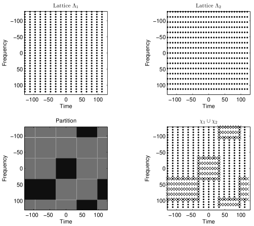
Figure 1. Partition in time-frequency and resulting quilted lattice

We now give a precise definition for quilted Gabor frames.

Definition 2 (Quilted Gabor frames).

Let Gabor frames $\mathcal{G}(g^{j},\Lambda^{j})_{j\in\mathcal{J}}$ for $\mathbf{L}^{2}(\mathbb{R}^{d})$ and an admissible covering $\Omega_{r}\subseteq(B_{R_{r}}(x_{r}))_{r\in\mathcal{I}}$ of $\mathbb{R}^{2d}$ be given. Define the local index sets $\mathcal{X}^{r}=\Omega_{r}\cap\Lambda^{m(r)}$, where $m:\mathcal{I}\mapsto\mathcal{J}$ is a mapping assigning a frame from the given Gabor frames to each member of the covering. Then the set

(4) $$\bigcup_{r\in\mathcal{I}}\mathcal{G}(g^{m(r)},\mathcal{X}^{r})$$

is called a quilted Gabor frame for $\mathbf{L}^{2}(\mathbb{R}^{d})$, if there exist constants $0<A,B<\infty$, such that

(5) $$A\|f\|_{2}^{2}\leq\sum_{r\in\mathcal{I}}\sum_{\lambda\in\mathcal{X}^{r}}|\langle f,\pi(\lambda)g^{m(r)}\rangle|^{2}\leq B\|f\|_{2}^{2}$$

holds for all $f\in\mathbf{L}^{2}(\mathbb{R}^{d})$.

The general setting of quilted frames includes, of course, various special cases. We first give some trivial examples which may however be relevant in applications.

Example 1.

For a given Gabor frame, we may choose additional sampling points in any selected region. This may be helpful, if in some applications, finer resolution is only desirable in certain parts of the time-frequency domain. Formally, this may be rephrased as follows. We are given Gabor frames $\mathcal{G}(g,\Lambda^{j})_{j\in\mathbb{N}}$ for $\mathbf{L}^{2}(\mathbb{R}^{d})$ with $\Lambda^{0}\subseteq\Lambda^{j}$ for $j\in\mathbb{N}$ and $A_{0}$ the lower frame bound for $j=0$. Then, for an admissible covering, the local index sets are defined by $\mathcal{X}^{r}=\Omega_{r}\cap\Lambda^{m(r)}$, where $m:\mathcal{I}\mapsto\mathbb{N}$ is the mapping selecting the local systems. It is then trivial to see, that the resulting quilted Gabor frame has a lower frame bound $A_{0}$. The existence of an upper frame bound is covered by Theorem 1.

Example 2.

For a given multi-window Gabor frame $\mathcal{G}(\{g_{1},\ldots,g_{n}\},\Lambda^{0})$, additional sampling points for selected windows may be added in certain parts of the time-frequency domain. For a formal description, assume that an admissible covering $\Omega_{r}$, $r\in\mathcal{I}$, is given and let $\Lambda^{0}\subseteq\Lambda^{j}$ for $j=1,\ldots,N$ as in the previous example. The mapping $m:\mathcal{I}\rightarrow\{0,\ldots,N\}^{n}$ is given by $m(r)(k)=0,\,k=1,\ldots,n$ whenever the original lattice is maintained for all windows in the support of $\Omega_{r}$ and by $m(r)(k)=j_{0},j_{0}\in\{1,\ldots,N\}$, if denser sampling correspondong to $\Lambda^{j_{0}}$ is desired in $\Omega_{r}$ for the window $g_{k}$.

In the next section we will prove the Bessel property of quilted systems obtained in a rather general situation, allowing for a finite overlap between the local patches. In the construction of lower frame bounds, a certain overlap between adjoint patches is often necessary. The two subsequent sections then describe two situations, in which a lower frame bound for the resulting quilted Gabor frame can be constructed explicitly.

4. The Bessel condition in the general case

We prove the existence of an upper frame bound for quilted frames as defined in (4). Note that the Bessel property alone allows for interesting conclusions about operators associated with the respective sequence, compare [2]. We will deduce the Bessel property of quilted Gabor frames from a general statement on relatively separated sampling sets. This result generalizes a result given in [26] on the Bessel property of irregular time-frequency shifts of a single atom. We prove that an arbitrary function from a set of window functions satisfying a common decay condition may be chosen for every sampling point in a relatively separated sampling set to obtain a Bessel sequence.

We assume that different given Gabor systems are to be used in compact sets $\Omega_{r}$ corresponding to the members of an admissible covering of $\mathbb{R}^{2d}$. Under the assumption that the windows under consideration satisfy a common decay condition in time-frequency and that the set of lattices is compact, we claim that an upper frame bound, or Bessel bound, can be found. As before, $g_{0}$ denotes the Gaussian window.

Theorem 1.

Let Gabor frames $\mathcal{G}(g^{j},\Lambda^{j})_{j\in\mathcal{J}}$ for $\mathbf{L}^{2}(\mathbb{R}^{d})$ and an admissible covering $\Omega_{r}\subseteq(B_{R_{r}}(x_{r}))_{r\in\mathcal{I}}$ of the signal domain be given. Assume further that

• $g^{j}\in H_{s,C}$ for all $j$, where

  $$H_{s,C}=\{g\in\mathbf{L}^{2}(\mathbb{R}^{d}):|\mathcal{V}_{g_{0}}g|(z)\leq C(1+\|z\|^{2})^{-\frac{s}{2}}\},\ s>2d,\ C>0.$$

• the lattice constants $\alpha^{j},\beta^{j}$ are chosen from a compact set in $\mathbb{R}^{+}\times\mathbb{R}^{+}$,
  i.e. $\alpha^{j}\subseteq[\alpha_{0},\alpha_{1}]\subset(0,\infty)$ and $\beta^{j}\subseteq[\beta_{0},\beta_{1}]\subset(0,\infty).$

• The regions assigned to the different Gabor systems correspond to an admissible covering $\Omega_{r},r\in\mathcal{I}$ with $\operatorname{supp}(\psi_{r})\subseteq\Omega_{r}\subseteq B_{R_{r}}(x_{r})$ for $r\in\mathcal{I}$.

Let $m:\mathcal{I}\mapsto\mathcal{J}$ be a mapping assigning a frame from $\mathcal{G}(g^{j},\Lambda^{j})_{j\in\mathcal{J}}$ to each member of the covering. Then for any $\delta<\infty$, the overall family given by

(6) $$\mathcal{G}^{Q}_{m}=\bigcup_{r\in\mathcal{I}}\{\pi(\lambda)g^{m(r)}:\lambda\in\mathcal{X}^{r}\subset\Lambda^{r},\ \mathcal{X}^{r}=\Lambda^{m(r)}\cap B_{R_{r}+\delta}\}$$

possesses an upper frame bound,  i.e., is a Bessel sequence for $\mathbf{L}^{2}(\mathbb{R}^{d})$.

Note that the theorem states that in particular the local systems given by $\mathcal{X}^{r}=\Omega_{r}\cap\Lambda^{m(r)}$ for all $r$ lead to a Bessel sequence. More generally, however, the local patches can uniformly be enlarged by a radius $\delta$.
We first prove a general statement on sampling of functions in certain Wiener amalgam spaces over relatively separate sampling sets.

Definition 3 (Relatively separated sets).

A set $\mathcal{X}=\{z_{i}=(x_{i},\xi_{i}),i\in\mathcal{I}\}$ in $\mathbb{R}^{2d}$ is called (uniformly) $\gamma$-separated, if $\inf_{j,k\in\mathcal{I},i\neq j}|z_{j}-z_{k}|=\gamma>0$. A relatively separated set is a finite union of separated sets. We call $\mathcal{X}$ $(\gamma,R)$-relative separated if the number of separated sets is $R$.

Remark 1.

It is easy to show that the concept of relative separation does not depend on the specific values of $\gamma$ and $R$. In other words, any $(\gamma,R)$-relative separated set is also a finite union of $\eta$-separated subsets. Of course one has to allow to compensate the smallness of $\eta$ by a larger number $R^{\prime}=R^{\prime}(\eta)$.
There is an equivalent point of view. A sequence is relatively separated in $R^{k}$ if and only if for some fixed $s>0$ the family $(B_{s}(x_{k}))_{k\geq 1}$ covers each point $x$ in $R^{k}$ at most $h=h(s)$ times, uniformly with respect to $x$.

Lemma 1.

Let $1\leq p<\infty$. Given a pair $(\gamma,R)$ there exists a constant $C=C(\gamma,R)$ such that for all $(\gamma,R)$-separated sets $\mathcal{X}$ and all functions $F\in{\boldsymbol{W}}(C^{0},\ell^{p})(\mathbb{R}^{2d})$ one has $F|_{\mathcal{X}}$ is in $\ell^{p}(\mathcal{X})$ and

(7) $$\|F|_{\mathcal{X}}\|_{\ell^{p}(\mathcal{X})}=\left(\sum_{x_{i}\in\mathcal{X}}|F(x_{i})|^{p}\right)^{1/p}\leq C\|F\|\ _{{\boldsymbol{W}}(C^{0},\ell^{p})}.$$

Proof:
Recall that $\|F\|_{{\boldsymbol{W}}(C^{0},\ell^{p})}=\|a_{kn}\|_{\ell^{p}}$, where

$$a_{kn}=\mathrm{esssup}_{(x,\xi)\in Q}|F(x+k,\xi+n)|=\|F\cdot T_{(k,n)}\chi_{Q}\|_{\infty}.$$

By assumption, $\mathcal{X}$ is the finite union of uniformly separated sets $\mathcal{X}^{r},r=1,\ldots,R$ and there exists $\gamma$, such that $\min|z_{j}-z_{k}|\geq\gamma>0$ for any pair $z_{j},z_{k}$ in $\mathcal{X}^{r}$, with $j\neq k$. Hence, for all $r=1,\ldots,R$, we have at most $(1+\frac{1}{\gamma})^{2d}$ points $z_{i}\in\mathcal{X}^{r}$ in the box $(k,n)+Q$, $(k,n)\in\mathbb{Z}^{d}\times\mathbb{Z}^{d}$, such that the number of $z_{i}\in\mathcal{X}$ in this box is bounded above by $R\cdot(1+1/{\gamma})$. Clearly

$$|F(x,\xi)|\leq\|F\cdot T_{(k,n)}\chi_{Q}\|_{\infty}\mbox{ for all }(x,\xi)\in(k,n)+Q.$$

Altogether, this yields:

(8) $$\sum_{z_{i}\in\mathcal{X}}|F(z_{i})|^{p}\ \leq\ \ R\cdot(1+\frac{1}{\gamma})^{2d}\sum_{(k,n)\in\mathbb{Z}^{2d}}\|F\cdot T_{(k,n)}\chi\|_{\infty}^{p}$$

$$=\ R\cdot(1+\frac{1}{\gamma})^{2d}\ \|F\|^{p}_{{\boldsymbol{W}}(C^{0},\ell^{p})}$$

$\square$

Remark 2.

Analogous statements are true in more general situations, especially for any weighted sequence space $\ell^{p}_{m}$, see [19, Lemma 3.8] for example.
The condition, that $F$ is continuous (locally in $C^{0}$), guarantees, that sampling is well-defined. Of course, weaker conditions, for example, semi-continuity, are sufficient.

The upper frame bound estimate will follow from a point wise estimate over the family of short-time Fourier transforms

(9) $$F(\lambda)=\sup_{j\in\mathcal{J}}|V_{g^{j}}f(\lambda)|,\quad\lambda\in\mathbb{R}^{2d}$$

We will make use of following lemma.

Lemma 2.

Assume that $g\in M\subseteq H_{s,C}$ for $s>2d$, $C>0$. Then there exists some constant $C>0$ such that for all $f\in\mathbf{L}^{2}(\mathbb{R}^{d})$ one has the following uniform estimate of $V_{g}f$ in ${\boldsymbol{W}}(C^{0},\ell^{2})$:

$$\|\sup_{g\in M}|V_{g}f|\|_{{\boldsymbol{W}}(C^{0},\ell^{2})}\quad\leq\quad C_{1}\|f\|_{2},\quad\mbox{ for all }f\in L^{2}.$$

Proof:
The crucial step is to invoke the convolution relation between different short-time Fourier transforms ([22, Lemma 11.3.3] ). For convenience in the application below let us denote the generic elements from $M$ by $g^{j}$ (instead of $g_{0}$ in 11.3.3), and make the choice $\gamma=g=g_{0}$, the normalized Gauss function $g_{0}$. Then obviously $\langle\gamma,g\rangle=\|g_{0}\|_{2}^{2}=1$ and we have the following estimate

$$|\mathcal{V}_{g^{j}}f(\lambda)|\leq\left[|\mathcal{V}_{g_{0}}f|\ast|\mathcal{V}_{g^{j}}g_{0}|\right](\lambda)$$

Since $|\mathcal{V}_{g^{j}}g_{0}(\lambda)|=|\mathcal{V}_{g_{0}}{g^{j}}(-\lambda)|\leq w_{s}(\lambda)$, we may take the pointwise supremum over $g^{j}\in M$ on the left side and arrive at

$$\sup_{g^{j}\in M}|\mathcal{V}_{g^{j}}f(\lambda)|\leq(|\mathcal{V}_{g_{0}}f|\ast Cw_{s})(\lambda)$$

Of course $s>2d$ implies that $w_{s}\in{\boldsymbol{W}}(C^{0},\ell^{1})(\mathbb{R}^{2d})$. Using the general fact ([22, Cor. 3.2.2] ) that $\|V_{g_{0}}f\|_{2}\leq C_{2}\|f\|_{2}$ for any $f\in\mathbf{L}^{2}(\mathbb{R}^{d})$ and applying the convolution relation $\mathbf{L}^{2}\ast{\boldsymbol{W}}(C^{0},\ell^{1})\subseteq{\boldsymbol{W}}(L^{1},\ell^{2})\ast{\boldsymbol{W}}(C^{0},\ell^{1})\subseteq{\boldsymbol{W}}(C^{0},\ell^{2})$, together with the appropriate estimates, we arrive at the desired estimate. $\square$

Remark 3.

It is worthwhile to note that the above result is not just a simple compactness argument. As a matter of fact it is not difficult to construct compact sets $M\subset S_{0}(\mathbb{R}^{d})$ for which the above result is not valid. One may, for example, just take a null sequence of the form $(c_{n}T_{x_{n}}g)_{n\geq 1}$ for some $g\in S_{0}(\mathbb{R}^{d})$, and with $(c_{n})\in C_{0}$ but $(c_{n})\notin\ell^{2}$.

The next theorem states that for a relatively separated sampling set of time-frequency shifts we can construct a Bessel sequence by associating to each sampling point an element from $H_{s,C}$. As before, we let $M\subseteq H_{s,C}$ be a set of window functions indexed by $\mathcal{J}$.

Theorem 2.

Let $\mathcal{X}=\{z_{i}=(x_{i},\xi_{i}),i\in\mathcal{I}\}$ in $\mathbb{R}^{2d}$ be a relatively separated set of sampling points in $\mathbb{R}^{2d}$. Let $m:\mathcal{X}\rightarrow\mathcal{J}$ be a mapping assigning a window $g^{m(z_{i})}\in M$ to each sampling point. Then the set

(10) $$\{\pi(z_{i})g^{m(z_{i})},i\in\mathcal{I}\}$$

is a Bessel Sequence for $\mathbf{L}^{2}(\mathbb{R}^{d})$.

Proof:
We have to estimate the series

$$\sum_{z_{i}\in\mathcal{X}}|\langle f,\pi(z_{i})g^{m(z_{i})}\rangle|^{2}=\sum_{z_{i}\in\mathcal{X}}|\mathcal{V}_{g^{m(z_{i})}}f(z_{i})|^{2}\leq\sum_{z_{i}\in\mathcal{X}}|F(z_{i})|^{2},$$

with $F$ given by (9). Now, as shown in the previous lemma, $F$ is in ${\boldsymbol{W}}(C^{0},\ell^{2})$. Hence, since $\mathcal{X}$ is a relatively separated set, Lemma 2 can be applied to obtain the following estimate for the Bessel bound of (10):

$$\sum_{z_{i}\in\mathcal{X}}|\langle f,\pi(z_{i})g^{m(z_{i})}\rangle|^{2}\leq C^{2}R(1+1/\gamma)^{2d}\|f\|^{2}_{2}$$

$\square$

Lemma 3.

The union of points $\{\lambda=(x,\xi),\lambda\in\mathcal{X}^{r}\}$ in the discrete sets $\mathcal{X}^{r}$ as chosen in Theorem 1 is relatively separated.

Proof:
Each of the lattices $\Lambda^{r}$ determining the Gabor frames used in the construction of $\mathcal{G}^{Q}_{m}$ is of course separated, even uniformly with respect to $r$. The admissibility condition for $(\Omega_{r})_{r\in\mathcal{I}}$ allows only finite overlap between any pair of members in the covering, or equivalently that the family of balls of radius $R_{r}$ centered at $x_{r}$ forms a covering of (uniformly) bounded height. By assumption, increasing each of the balls $B_{R_{r}}(x_{r})$ by the finite radius $\delta>0$, only the height of the covering will be increased, but not the property of (uniformly) finite height. In other words, the family of enlarged balls $B_{R_{r}+\delta}(x_{r})$ is still an admissible covering of ${\mathbb{R}^{d}}$ and the union of the $\mathcal{X}$ is a relatively separated set. $\square$

We conclude the proof of Theorem 1 by choosing $M=\{g^{j},j\in\mathcal{J}\}$ in the following Corollary.

Corollary 1.

An upper frame bound for $\mathcal{G}^{Q}_{m}$ as defined in (6) is given by $C^{2}n(\delta)(1+1/\gamma)^{2d}$.

Note that $n(\delta)$ denotes the height of the covering, which depends on $\delta$.

5. Reduced multi-window Gabor frames: windows with compact support or bandwidth

In this section, we show that in a specific situation, which is, however, of practical relevance, quilted Gabor frames may be constructed. In the present model, we only change the resolution in time (or frequency). This means, that the time-frequency domain is partitioned into stripes rather than patches. Under the additional assumption that the analysis window has compact support (or bandwidth), we easily obtain a lower frame bound for the quilted system.

Assume that we are given Gabor frames $\mathcal{G}(g^{j},\Lambda^{j})$ for $\mathbf{L}^{2}(\mathbb{R}^{d})$, $j\in\mathcal{J}$, where all the windows $g^{j}$ have compact support and $\|g^{j}\|_{S_{0}}\leq C_{g}<\infty\,\forall j$. We now want to use each system for a certain time, i.e., in a restricted stripe in the time-frequency domain. The stripes are defined by means of a partition of unity: we assume that $f=\sum_{r\in\mathcal{I}}\psi_{r}f$ with $\psi_{r}\leq 1$ and that the $\psi_{r}$ have compact support in $[a_{r},b_{r}]$. By means of a mapping $m:\mathcal{I}\rightarrow\mathcal{J}$, we assign one particular frame to each of these stripes.

Now, subfamilies of the given Gabor frames may be constructed as follows. Assume, for simplicity, that $m(0)=0$ and consider the task to represent $\psi_{0}f$ in terms of the given Gabor frame $\mathcal{G}(g^{0},\Lambda^{0})$:

$$\psi_{0}f= \psi_{0}(\sum_{\lambda\in\Lambda^{0}}\langle f,\pi(\lambda)g^{0}\rangle\pi(\lambda)g^{0})$$

$$= \sum_{\lambda\in\Lambda^{0}}\langle f,\pi(\lambda)g^{0}\rangle\psi_{0}\pi(\lambda)g^{0}.$$

Now, there exist $n^{u}_{0}$ and $n^{l}_{0}$ such that for $\lambda=(n\alpha_{0},m\beta_{0})$ with $n\notin[n^{l}_{0},n^{u}_{0}]$, we find that $\psi_{0}\pi(\lambda)g^{0}\equiv 0$, hence

$$\psi_{0}f=\sum_{\lambda\in\mathcal{X}_{0}}\langle f,\pi(\lambda)g^{0}\rangle\psi_{0}\pi(\lambda)g^{0},$$

where $\mathcal{X}_{0}=[n^{l}_{0}\cdot\alpha_{0},n^{u}_{0}\cdot\alpha_{0}]\times\beta_{0}\mathbb{Z}$ is the subset of $\Lambda^{0}$ corresponding to the nonzero contributions.

Analogously subsets $\mathcal{X}_{r}\subset\Lambda^{m(r)}$ are chosen for all $r$, and we obtain:

(11) $$f=\sum_{r\in\mathcal{I}}\psi_{r}f=\sum_{r}\sum_{\lambda\in\mathcal{X}^{r}}\langle f,\pi(\lambda)g^{m(r)}\rangle\psi_{r}\pi(\lambda)g^{m(r)}.$$

With this construction, we state the following proposition.

Proposition 1.

For a family of tight Gabor frames $\mathcal{G}(g^{j},\Lambda^{j})$, $j\in\mathcal{J}$, for $\mathbf{L}^{2}(\mathbb{R}^{d})$ let $\sup_{j\in\mathcal{I}}\|g^{j}\|_{S_{0}}=C_{g}<\infty$ and $C_{\Lambda^{j}}=(\frac{1}{\alpha_{j}}+1)^{d}(\frac{1}{\beta_{j}}+1)^{d}\leq C_{\Lambda}<\infty$ for all $j\in\mathcal{J}$. Let a partition of unity $(\psi_{r})_{r\in\mathcal{I}}$ of compactly supported $\psi_{r}$ with height $n_{0}$ be given and let a mapping $m:\mathcal{I}\rightarrow\mathcal{J}$ assign a frame $\mathcal{G}(g^{m(r)},\Lambda^{m(r)})$ to each $r\in\mathcal{I}$. Assume that index sets $\mathcal{X}^{r}=[n^{l}_{r}\cdot\alpha_{m(r)},n^{u}_{r}\cdot\alpha_{m(r)}]\times\beta_{m(r)}\mathbb{Z}$ are chosen such that for all $r\in\mathcal{I}$ and $\lambda=(n\alpha_{m(r)},m\beta_{m(r)})$ with $n\notin[n^{l}_{m(r)},n^{u}_{m(r)}]$, we have that $\psi_{r}\pi(\lambda)g^{m(r)}\equiv 0$.
Then, the union of the subfamilies $\bigcup_{r\in\mathcal{I}}(g^{m(r)},\mathcal{X}_{r})$ is a frame for $\mathbf{L}^{2}(\mathbb{R}^{d})$ with a lower frame bound given by $1/(n_{0}C_{\Lambda}C^{2}_{g})$.

Proof:
First note that

(12) $$\|\psi_{r}h\|_{2}^{2}\leq\|h\|_{2}^{2}\ \mbox{ for all }\ h\in\mathbf{L}^{2}(\mathbb{R}^{d})$$

Now set $h_{r}=\sum_{\lambda\in\mathcal{X}^{r}}\langle f,\pi(\lambda)g^{m(r)}\rangle\pi(\lambda)g^{m(r)}$ and thus, with (12):

$$\|f\|_{2}^{2}\leq n_{0}\sum_{r}\|\psi_{r}f\|_{2}^{2}$$

$$= n_{0}\sum_{r}\|\sum_{\lambda\in\mathcal{X}^{r}}\langle f,\pi(\lambda)g^{m(r)}\rangle\psi_{r}\pi(\lambda)g^{m(r)}\|_{2}^{2}$$

$$= n_{0}\sum_{r}\|h_{r}\psi_{r}\|_{2}^{2}\leq n_{0}\sum_{r}\|\sum_{\lambda\in\mathcal{X}^{r}}\langle f,\pi(\lambda)g^{m(r)}\rangle\pi(\lambda)g^{m(r)}\|_{2}^{2}$$

$$\leq n_{0}\sum_{r}(\frac{1}{\alpha_{j}}+1)^{d}(\frac{1}{\beta_{j}}+1)^{d}\|g^{m(r)}\|^{2}_{S_{0}}\sum_{\lambda\in\mathcal{X}^{r}}|\langle f,\pi(\lambda)g^{m(r)}\rangle|^{2}$$

$$\leq n_{0}C_{\Lambda}C^{2}_{g}\sum_{r}\sum_{\lambda\in\mathcal{X}^{r}}|\langle f,\pi(\lambda)g^{m(r)}\rangle|^{2}$$

The last inequality is due to the boundedness of the frame-synthesis operator $T^{\ast}_{g^{m(r)}}:\ell^{2}(\Lambda^{j})\rightarrow\mathbf{L}^{2}(\mathbb{R}^{d})$, whenever the window $g^{m(r)}$ is in $S_{0}(\mathbb{R}^{d})$, see [22, Proposition 6.2.2]. This proves the existence of a lower frame bound as stated. The existence of an upper frame bound can be seen directly from the construction of the subfamilies, and is furthermore covered by the general case proved in Section 4. $\square$

Remark 4.

1. An analogous statement holds for general, not necessarily tight frames, for, if $\gamma^{j}$ are the dual windows for each $g^{j}$, then $\|S_{j}^{-1}g^{j}\|\leq\frac{1}{A_{j}}\|g^{j}\||$.

2. The same construction may be realized in the Fourier transform domain by applying a partition of unity to $\hat{f}$. This corresponds to the usage of different Gabor frames in different stripes of the frequency domain and hence resembles a non-orthogonal filter bank. As a particular example, a constant-Q transform may be realized [5].

3. Note that a similar yet more restrictive construction, corresponding to the classical “painless non-orthogonal expansions” was suggested in [24]. Very recently, another related and highly interesting construction has been suggested in [28].

6. Replacing a finite number of frame elements

We now consider the task of replacing a finite number of atoms from a given (Gabor) frame by a finite number of atoms from a different (Gabor) frame. The following theorem gives a condition valid for general frames, which will then be applied to Gabor frames. Recall, that $T_{g}$ and $T_{g}^{\ast}$ denote the analysis and synthesis mapping, respectively, for given $g$ and $\Lambda$. In this section, we use the notation $T_{g,\mathcal{I}}$ and $T^{\ast}_{g,\mathcal{I}}$ for the respective mappings corresponding to subsets of the given lattices. For example, let $\mathcal{F}_{1}\subset\Lambda$ be a finite subset of a lattice $\Lambda$, then $T_{g,\mathcal{F}_{1}}(f)=\langle f,\pi(\lambda)g\rangle$, for $\lambda\in\mathcal{F}_{1}$. The theorem makes use of a linear mapping $L$ describing the replacement procedure in the coefficient domain. As long as elements from frame $\mathcal{G}_{1}$ may be replaced by elements from $\mathcal{G}_{2}$ in a controlled manner, i.e. without loosing energy, a quilted frame can be obtained.

Theorem 3.

Assume that two frames $\mathcal{G}_{1}=\{g_{i},i\in\mathcal{I}\}$ and $\mathcal{G}_{2}=\{h_{j},j\in\mathcal{J}\}$ for $\mathbf{L}^{2}(\mathbb{R}^{d})$ are given and a finite number of elements $\{g_{i},i\in\mathcal{F}_{1}\subset\mathcal{I}\}$ of $\mathcal{G}_{1}$ are to be replaced by a finite number of elements $\{h_{j},j\in\mathcal{F}_{2}\subset\mathcal{J}\}$ of $\mathcal{G}_{2}$.
Let $A_{1}$ be the lower frame-bound of $\mathcal{G}_{1}$. If a bounded linear mapping $L:\ell^{2}(\mathcal{F}_{1})\mapsto\ell^{2}(\mathcal{F}_{2})$ can be found such that

(13) $$\|T^{\ast}_{g,\mathcal{F}_{1}}-T^{\ast}_{h,\mathcal{F}_{2}}L\|_{2}^{2}=C<\frac{A_{1}}{2},$$

then the set

(14) $$\{g_{i},i\in\mathcal{I}\backslash\mathcal{F}_{1}\}\cup\{h_{j},j\in\mathcal{F}_{2}\}$$

is a frame for $\mathbf{L}^{2}(\mathbb{R}^{d})$ with a lower frame bound given by $(A_{1}-2C)/\max(1,2\|L^{\ast}\|_{2}^{2})$.

Proof:
First note that

$$A_{1}\|f\|_{2}^{2}\leq\sum_{i\in\mathcal{I}\backslash\mathcal{F}_{1}}|\langle f,g_{i}\rangle|^{2}+\sum_{i\in\mathcal{F}_{1}}|\langle f,g_{i}\rangle|^{2}=\|T_{g,\mathcal{I}\backslash\mathcal{F}_{1}}\|_{2}^{2}+\|T_{g,\mathcal{F}_{1}}\|_{2}^{2}.$$

Now, we have

$$\|T_{g,\mathcal{F}_{1}}\|_{2}^{2} \leq(\|(T_{g,\mathcal{F}_{1}}-L^{\ast}T_{h,\mathcal{F}_{2}})f\|+\|L^{\ast}T_{h,\mathcal{F}_{2}}f\|)^{2}$$

$$\leq 2\cdot\|(T_{g,\mathcal{F}_{1}}-L^{\ast}T_{h,\mathcal{F}_{2}})f\|_{2}^{2}+2\cdot\|L^{\ast}T_{h,\mathcal{F}_{2}}\|_{2}^{2}$$

$$\leq 2\cdot C\cdot\|f\|_{2}^{2}+2\cdot\|L^{\ast}T_{h,\mathcal{F}_{2}}f\|_{2}^{2},$$

hence

$$(A_{1}-2C)\|f\|_{2}^{2} \leq\|T_{\mathcal{I}\backslash\mathcal{F}_{1}}f\|_{2}^{2}+2\cdot\|L^{\ast}\|_{2}^{2}\|T_{h,\mathcal{F}_{2}}f\|_{2}^{2}$$

$$\leq\max(1,2\|L^{\ast}\|_{2}^{2})\cdot(\sum_{i\in\mathcal{I}\backslash\mathcal{F}_{1}}|\langle f,g_{i}\rangle|^{2}+\sum_{j\in\mathcal{F}_{2}}|\langle f,h_{j}\rangle|^{2})$$

and hence $(A_{1}-2C)/\max(1,2\|L^{\ast}\|_{2}^{2})$ is a lower frame bound for the system given in (14). The existence of an upper frame bound is trivial. $\square$
Note that the above theorem only states the existence of a lower frame bound under the given conditions, while this frame bound will usually not be optimal.
We now turn to the special case of Gabor frames.

Corollary 2.

Assume that tight Gabor frames $\mathcal{G}(g,\Lambda^{1})$ and $\mathcal{G}(h,\Lambda^{2})$ with $g,h\in S_{0}(\mathbb{R}^{d})$ are given. Assume further that in a compact region $\Omega\subset\mathbb{R}^{2d}$ the time-frequency shifted atoms $\pi(\lambda)g$, $\lambda\in\mathcal{F}_{1}=\Omega\cap\Lambda^{1}$ are to be replaced by a finite set of time-frequency shifted atoms $\pi(\mu)h$, $\mu\in\mathcal{F}_{2}\subset\Lambda^{2}$.

• If $\Lambda^{1}=\Lambda^{2}$, then

  (15) $$\mathcal{G}=\{\pi(\lambda)g:\lambda\in\Lambda\setminus\mathcal{F}_{1}\}\cup\{\pi(\mu)h:\mu\in\mathcal{F}_{2}\}$$

  is a (quilted Gabor) frame for $\mathbf{L}^{2}(\mathbb{R}^{d})$, whenever

  $$\|h-g\|_{S_{0}}^{2}\ =C<\frac{A_{1}}{2C_{\Lambda}},$$

  where $C_{\Lambda}$ is a constant only depending on the lattice $\Lambda=\Lambda^{1}=\Lambda^{2}$.

• For general $\Lambda^{2}$, a compact set $\Omega^{\ast}$ in $\mathbb{R}^{2d}$ can be chosen such that for $\mathcal{F}_{2}=\Omega^{\ast}\cap\Lambda^{2}$, the union

  (16) $$\mathcal{G}=\{\pi(\lambda)g:\lambda\in\Lambda^{1}\setminus\mathcal{F}_{1}\}\cup\{\pi(\mu)h:\mu\in\mathcal{F}_{2}\}$$

  is a (quilted Gabor) frame.

Proof:
Statement (a) can easily be seen by choosing $L=\operatorname{Id}$ in Theorem 3:

$$\|T_{\mathcal{F}_{1}}^{\ast}-T_{\mathcal{F}_{1}}^{\ast}\|^{2}_{\ell^{2}\mapsto\mathbf{L}^{2}(\mathbb{R}^{d})} =\sup_{\|c\|_{2}=1}\|\sum_{\lambda\in\mathcal{F}_{1}}c_{\lambda}(\pi(\lambda)g-\pi(\lambda)h)\|^{2}_{2}$$

$$\leq C_{\Lambda}\cdot\|h-g\|_{S_{0}}^{2},$$

where the last inequality follows from boundedness of the synthesis operator for windows in $S_{0}$, [22, Theorem 12.2.4].
To show (b), we first introduce the mapping $L:\ell^{2}(\mathcal{F}_{1})\mapsto\ell^{2}(\mathcal{F}_{2})$ as follows. For a finite sequence $\mathbf{c}=(c_{\lambda})_{\lambda\in\mathcal{F}_{1}}$ we define $L(\mathbf{c})(\mu)=(\langle\sum_{\lambda\in\mathcal{F}_{1}}c_{\lambda}\pi(\lambda)g,\pi(\mu)h\rangle)_{\mu\in\mathcal{F}_{2}}$, for which

$$\|L\|_{\ell^{2}(\mathcal{F}_{1})\mapsto\ell^{2}(\mathcal{F}_{2})}^{2} =\sup_{\|c\|_{2}=1}\sum_{\mu\in\mathcal{F}_{2}}|\sum_{\lambda\in\mathcal{F}_{1}}c_{\lambda}\langle\pi(\lambda)g,\pi(\mu)h\rangle|^{2}$$

$$=\|T_{h,\mathcal{F}_{2}}T^{\ast}_{g,\mathcal{F}_{1}}\|_{2}^{2}\leq C_{\Lambda^{1}}C_{\Lambda^{2}}\cdot\|g\|_{S_{0}}^{2}\|h\|_{S_{0}}^{2}$$

due to the boundedness of synthesis and analysis operator, $T_{h,\mathcal{F}_{2}}$ and $T^{\ast}_{g,\mathcal{F}_{1}}$, respectively. We then have:

$$\|T_{\mathcal{F}_{1}}^{\ast}-T_{\mathcal{F}_{2}}^{\ast}L\|_{\ell^{2}\mapsto\mathbf{L}^{2}(\mathbb{R}^{d})} =\sup_{\|c\|_{2}=1}\|\sum_{\lambda\in\mathcal{F}_{1}}c_{\lambda}\pi(\lambda)g-\sum_{\mu\in\mathcal{F}_{2}}\sum_{\lambda\in\mathcal{F}_{1}}\langle c_{\lambda}\pi(\lambda)g,\pi(\mu)h\rangle\pi(\mu)h\|_{2}$$

$$=\sup_{\|c\|_{2}=1}\|\sum_{\mu\in\mathcal{F}_{2}^{c}}\sum_{\lambda\in\mathcal{F}_{1}}c_{\lambda}\langle\pi(\lambda)g,\pi(\mu)h\rangle\pi(\mu)h\|_{2}$$

$$\leq\|h\|_{2}\sup_{\|c\|_{2}=1}\sum_{\mu\in\mathcal{F}_{2}^{c}}\sum_{\lambda\in\mathcal{F}_{1}}|c_{\lambda}|\cdot|\mathcal{V}_{g}h(\mu-\lambda)|$$

$$\leq\|h\|_{2}\sqrt{|\mathcal{F}_{1}|}\sum_{\mu\in\mathcal{F}_{2}^{c}}\max_{\lambda\in\mathcal{F}_{1}}|\mathcal{V}_{g}h(\mu-\lambda)|$$

where $\mathcal{F}_{2}^{c}=\Lambda^{2}\backslash\mathcal{F}_{2}$. Now an appropriate set $\mathcal{F}_{2}$ may be constructed as follows:
Let $G=|\mathcal{V}_{g}h|\in{\boldsymbol{W}}(C^{0},\ell^{1})$. We can choose a compact set $\Omega^{\ast}\subset\mathbb{R}^{2d}$, such that

$$\|\max_{\lambda\in\mathcal{F}_{1}}(T_{\lambda}G-(T_{\lambda}G)\cdot\chi_{\Omega^{\ast}})\|_{W}<\tilde{\varepsilon}=\frac{\sqrt{A_{1}}}{\sqrt{2|\mathcal{F}_{1}|}\|h\|_{2}C_{\Lambda^{2}}},$$

where $\chi_{\Omega^{\ast}}$ is the indicator function of the set $\Omega$. Now set

$$\mathcal{F}_{2}=\Lambda^{2}\cap\Omega^{\ast},$$

then

$$\sum_{\mu\in\mathcal{F}_{2}^{c}}\max_{\lambda\in\mathcal{F}_{1}}T_{\lambda}G(\mu) =\|(\max_{\lambda\in\mathcal{F}_{1}}T_{\lambda}G)\big{|}_{\mathcal{F}_{2}^{c}}\|_{\ell^{1}}$$

$$=\|\max_{\lambda\in\mathcal{F}_{1}}(T_{\lambda}G-T_{\lambda}G\cdot\chi_{\Omega^{\ast}})\big{|}_{\Lambda^{2}}\|_{\ell^{1}}$$

(17) $$\leq C_{\Lambda^{2}}\cdot\|(T_{\lambda}G-T_{\lambda}G\cdot\chi_{\Omega^{\ast}})\|_{{\boldsymbol{W}}(C^{0},\ell^{1})}$$

$$\leq C_{\Lambda^{2}}\cdot\tilde{\varepsilon}=C_{\Lambda^{2}}\cdot\frac{\sqrt{A_{1}}}{\sqrt{2|\mathcal{F}_{1}|}\|h\|_{2}C_{\Lambda^{2}}},$$

where we used Lemma 1 in (17). Hence, $\mathcal{F}_{2}$ can be chosen, such that

$$\|T_{\mathcal{F}_{1}}^{\ast}-T_{\mathcal{F}_{2}}^{\ast}L\|^{2}_{\ell^{2}\mapsto\mathbf{L}^{2}(\mathbb{R}^{d})}<A_{1}/2.$$

Of course, the existence of an upper frame bound is trivial and the resulting system (16) is a quilted Gabor frame according to Theorem 3. $\square$

Remark 5.

(1) The size of the region in which atoms from $\mathcal{G}_{1}$ have to be replaced, influences the choice of $\Omega^{\ast}$. In particular, $\tilde{\varepsilon}$ is reciprocally related to $\sqrt{|\mathcal{F}_{1}|}$, i.e., $\Omega^{\ast}$ grows in dependence on the perimeter rather than the area of $\Omega$.
(2) For statement (a) in Corollary 2, if $g,h\in\mathbf{L}^{2}(\mathbb{R}^{d})$, then the frame property follows whenever

$$\|h-g\|_{2}^{2}\ =C<A_{1}/(2|\mathcal{F}_{1}|).$$

Note that the size of $\Omega$ determines the necessary similarity of the windows, whereas, for windows in $S_{0}(\mathbb{R}^{d})$, the good localization implied by $S_{0}$-membership allows for a stronger statement.
(3) The construction in Corollary 2 implies explicit dependence on time and frequency of the resulting quilted frame. Similarly, Gabor atoms in finitely many compact areas can be replaced by different Gabor systems. Details on this procedure will be reported elsewhere. From an application point of view, this process corresponds to finding optimal representations for local signal components, e.g. in the sense of sparsity.
(4) In Example 1, the linear mapping $L:\Lambda^{0}\rightarrow\bigcup_{r}\mathcal{X}^{r}$ can be chosen as follows:

$$L(c)(\lambda)=\begin{cases}c_{\lambda},&\mbox{for }\;\;\lambda\in\Lambda^{0}\\ 0,&\mbox{for}\;\;\lambda\in\bigcup_{r}\mathcal{X}^{r}\backslash\Lambda^{0}\end{cases}.$$

Then

$$\|T_{\Lambda^{0},g}^{\ast}-T_{\bigcup_{r}\mathcal{X}^{r},g}^{\ast}L\|^{2}=\sup_{\|c\|_{2}=1}\|\sum_{\lambda\in\Lambda^{0}}c_{\lambda}\pi(\lambda)g-\sum_{\lambda\in\bigcup_{r}\mathcal{X}^{r}}L(c)(\lambda)\pi(\lambda)g\|^{2}_{2}=0.$$

As underlined by Example 1 and Corollary 2(a), in constructing quilted Gabor frames, technically difficult situations mainly arise if the lattices and the windows vary.

7. Reconstruction and Simulations

Since the frame property has been proved for systems as described in Proposition 1 and Corollary 2, reconstruction can always be performed by means of a dual frame. However, since quilted Gabor frames possess a strong local structure, alternative and numerically cheaper methods may be preferable as long as sufficient precision in the reconstruction may be guaranteed. The next two sections present numerical results for various approaches to reconstruction for which the calculation of an exact dual frame is not necessary.

7.1. Reduced multi-window Gabor frames

We first consider reduced multi-window Gabor frames. Here, equation (11) yields an immediate reconstruction formula by means of projections onto the members of the partition of unity. However, we are more interested in the generic reconstruction by means of dual frames. We may compare the dual frame corresponding to the quilted Gabor frame $\bigcup_{j\in\mathcal{I}}(g^{j},\mathcal{X}_{j})$ with the quilted system $\bigcup_{j\in\mathcal{I}}(\gamma_{j},\mathcal{X}_{j})$ resulting from using the dual windows $\gamma_{j}$ of the original frames $\mathcal{G}_{j}$. Alternatively, we may start with tight Gabor frames.
While this approach does not result in perfect reconstruction in one step, we apply the frame algorithm (see [22, Chapter 5]) to obtain near-perfect reconstruction in a few iteration steps. In this context, the condition number of the operators involved plays an important role and depends on the amount of overlap that we introduce in the design of the system. In the following example, it turns out that, while no essential overlap is necessary to obtain a frame in the finite discrete case, the overlap as requested in the proof of Proposition 1 leads to faster convergence of the frame algorithm.

Example 3.

We consider two tight Gabor frames for $\mathbb{C}^{L}$ and $L=144$ and two cases of different redundancy. First, redundancy is $4.5$, corresponding to the lattices $\Lambda^{1}$ with $a=4,b=8$ and $\Lambda^{2}$ with $a=8,b=4$. Second, we consider two frames with redundancy $1.125$, corresponding to the lattices $\Lambda^{1}$ with $a=8,b=16$ and $\Lambda_{2}$ with $a=16,b=8$. The corresponding tight windows are shown in Figure 2.

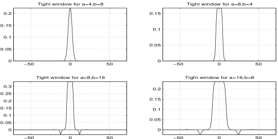
Figure 2. Tight windows corresponding to four different Gabor frames

We next generate a quilted Gabor system without overlap and a corresponding Gabor system with overlap, for both cases of redundancy. Note that in each lattice point as depicted in Figure 3, the tight window of the original Gabor frame is used.

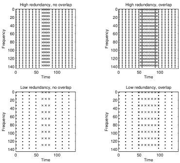
Figure 3. Various lattices with different amounts of overlap

We now look at the condition numbers of the resulting quilted systems, listed in Table 1.

Table 1: Condition number of four quilted Gabor frames Redundancy No overlap Overlap $4.5$ $1.6$ $1.4$ $1.125$ $6.4$ $1.5$

It is obvious, that higher redundancy leads to more stability in the process of quilting frames. On the other hand, for the system with low redundancy, overlap becomes essential in order to obtain acceptable condition numbers. These observations are consistently confirmed by more extensive numerical experiments.
In a next step, we now compare the convergence of the (iterative) frame algorithm for the $4$ cases considered in this example. Table 2 gives the number of iterations necessary to attain the threshold of $10^{-8}$. Figure 4 then shows the rate of convergence for the three cases with acceptable conditions numbers.

Table 2: Number of iterations for convergence of frame algorithm Redundancy No overlap Overlap $4.5$ $21$ $17$ $1.125$ $322$ $18$

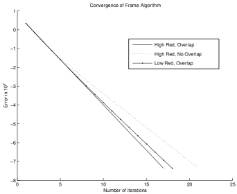
Figure 4. Convergence of frame algorithm

We finally discuss the following, “preconditioned” version of reconstruction for the case of low redundancy with overlap. We wish to reconstruct a random signal $r\in\mathbb{C}^{L}$ from its quilted Gabor coefficient. As a first guess, instead of calculating the dual frame of the quilted frame, we simply use the quilted tight frame for reconstruction: Let $T_{\mathcal{G}^{t}_{q}}$ denote the analysis operator corresponding to the quilted tight frame $\mathcal{G}^{t}_{q}=\bigcup_{j=1}^{2}(h_{j},\mathcal{X}_{j})$, where $h_{j}$ are the tight windows. We then obtain a reconstruction $rec$ by

$$rec=T_{\mathcal{G}^{t}_{q}}^{\ast}\cdot T_{\mathcal{G}^{t}_{q}}\cdot r.$$

Obviously, the result is not accurate and in particular in the regions of transition between the two systems, errors occur. However, we can correct a considerable amount of the deviation from the identity by simply pre-multiplying the frame-operator by the inverse of its diagonal. Hence, let $D$ be the diagonal matrix with $D(n,n)=T_{\mathcal{G}^{t}_{q}}^{\ast}\cdot T_{\mathcal{G}^{t}_{q}}(n,n)$, $n=1,\ldots,144$.

$$rec=T_{\mathcal{G}^{t}_{q}}^{\ast}\cdot T_{\mathcal{G}^{t}_{q}}\cdot D^{-1}\cdot r.$$

The respective results are shown in Figure 5. The relative error, defined by $\varepsilon=\frac{\|rec-r\|}{\|r\|}$ is then $0.2239$ for the uncorrected case and $0.032$ for the corrected version.

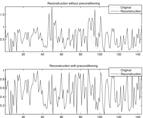
Figure 5. Reconstructed random signal

7.2. Replacing a finite number of elements

In our next example we consider a situation similar to the one discussed in Example 3, however, this time we wish to replace elements from $\mathcal{G}_{1}$ in a bounded, quadratic region of the time-frequency plane.

Example 4.

We consider the same Gabor frames as in Example 3, and look at the high redundancy systems first. As before, we compare the condition number of the system obtained with overlap to the less redundant situation. The two situations are shown in Figure 6. The quilted Gabor frame without overlap has condition number $1.5$, while allowing for some overlap, as shown in the second display of Figure 6 leads to condition number $1.4$. Accordingly, $18$ and $17$ iterations are necessary for convergence of the frame operator.
We now turn to the systems with low redundancy. Here we compare three amounts of overlap as shown in the upper displays of Figure 7. The condition numbers of the resulting systems and the convergence behavior of the corresponding frame algorithm are shown in the lower display of the same figure. Again, it becomes obvious that for low-redundancy systems, overlap is essential in order to obtain fast convergence in iterative reconstruction. On the other hand, increasing overlap beyond a certain amount, does not dramatically improve the condition numbers.

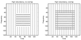
Figure 6. Replacing atoms with and without overlap, high redundancy

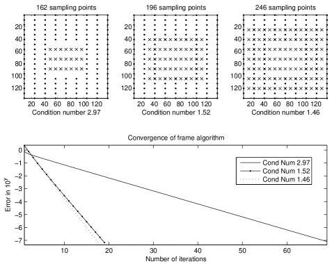
Figure 7. Replacing atoms with and without overlap, low redundancy

8. Summary and Outlook

We have shown the existence of a lower frame bound for two particular instances of quilted Gabor frames. Furthermore, an upper frame bound has been constructed for the general setting. We showed how to reconstruct signals from the coefficients obtained with quilted Gabor frames and numerical simulations have been provided.
Future work will mainly include the construction of lower frame bounds for more general situations. In particular, Proposition 1 will be generalized to Gabor frames with non-compactly supported windows. Furthermore, numerical simulations suggest that atoms from a given Gabor frame may be replaced by atoms from a different frame in infinitely many compact regions of the time-frequency plane under certain conditions. On the other hand, for practical applications algorithms applicable for long signals (number of sampling points $\gg 44100$) have to be developed. The results of processing with quilted Gabor frames will be assessed on the basis of real-life data. Preconditioning similar to the procedure suggested in Example 3 can be developed for the more complex situations of quilted frames, compare [3].

9. Acknowledgments

The author wishes to thank Hans Feichtinger for the joint development of the notion of quilted frames as well as innumerable discussions on the topic, his proofreading and invaluable comments on the content of this article. She also wishes to thank Franz Luef for his comments on an earlier version of the paper and Patrick Wolfe for fruitful scientific exchange on the topic of adaptive frames from the point of view of applications.

References

- [1] A. Aldroubi, C. Cabrelli, and U. Molter. Wavelets on Irregular Grids with Arbitrary Dilation Matrices, and Frame Atoms for L2(Rd). Appl. Comput. Harmon. Anal., Special Issue on Frames II.:119–140, 2004.
- [2] P. Balazs. Basic definition and properties of Bessel multipliers. J. Math. Anal. Appl., 325(1):571–585, 2007.
- [3] P. Balazs, H. G. Feichtinger, M. Hampejs, and G. Kracher. Double preconditioning for Gabor frames. IEEE Trans. Signal Process., 54(12):4597–4610, December 2006.
- [4] R. Bernardini and J. Kovacevic. Arbitrary tilings of the time-frequency plane using local bases. IEEE Trans. Signal Proc., 47(8):2293–2304, August 1999.
- [5] J. Brown. Calculation of a constant Q spectral transform. J. Acoust. Soc. Amer., 89(1):425 434, 1991.
- [6] P. G. Casazza and G. Kutyniok. Frames of subspaces. In Wavelets, Frames and Operator Theory, volume 345 of Contemp. Math., pages 87–113. Amer. Math. Soc., 2004.
- [7] P. G. Casazza, G. Kutyniok, and S. Li. Fusion frames and Distributed Processing. Appl. Comput. Harmon. Anal., 25(1):114–132, 2008.
- [8] O. Christensen. An introduction to frames and Riesz bases. Applied and Numerical Harmonic Analysis. Birkhäuser Boston Inc., Boston, MA, 2003.
- [9] L. Daudet and B. Torrésani. Hybrid representations for audiophonic signal encoding. Signal Process., 82(11):1595–1617, 2002.
- [10] M. Dörfler. Time-frequency Analysis for Music Signals. A Mathematical Approach. Journal of New Music Research, 30(1):3–12, 2001.
- [11] M. Dörfler. Gabor Analysis for a Class of Signals called Music. PhD thesis, University of Vienna, 2002.
- [12] M. Dörfler, H. G. Feichtinger, and K. Gröchenig. Time-Frequency Partitions for the Gelfand Triple . Math. Scand., 98(1):81–96, 2006.
- [13] M. Dörfler and K. Gröchenig. Time-Frequency partitions and characterizations of modulations spaces with localization operators. preprint, December 2009.
- [14] H. Feichtinger and P. Groebner. Banach spaces of distributions defined by decomposition methods. I. Math. Nachr., 123:97–120, 1985.
- [15] H. Feichtinger and G. Zimmermann. A Banach space of test functions for Gabor analysis. In H. and T. Strohmer, editors, Gabor Analysis and Algorithms: Theory and Applications, pages 123–170. Birkhäuser, Boston, 1998. Chap. 3.
- [16] H. G. Feichtinger. Banach spaces of distributions defined by decomposition methods, II. Math. Nachr., 132:207–237, 1987.
- [17] H. G. Feichtinger. Wiener amalgams over Euclidean spaces and some of their applications. In K. Jarosz, editor, Function Spaces, Proc Conf, Edwardsville/IL (USA) 1990, volume 136 of Lect. Notes Pure Appl. Math., pages 123–137. Marcel Dekker, 1992.
- [18] H. G. Feichtinger and P. Gröbner. Banach spaces of distributions defined by decomposition methods, I. Math. Nachr., 123:97–120, 1985.
- [19] H. G. Feichtinger and K. Gröchenig. Banach spaces related to integrable group representations and their atomic decompositions. I. J. Functional Anal., 86(2):307–340, 1989.
- [20] H. G. Feichtinger and T. Strohmer. Gabor Analysis and Algorithms. Theory and Applications. Birkhäuser, 1998.
- [21] M. Fornasier. Quasi-orthogonal decompositions of structured frames. J. Math. Anal. Appl., 289(1):180–199, 2004.
- [22] K. Gröchenig. Foundations of Time-Frequency Analysis. Appl. Numer. Harmon. Anal. Birkhäuser Boston, 2001.
- [23] C. Heil. An introduction to Wiener amalgams. In M. Krishna, R. Radha, and S. Thangavelu, editors, Wavelets and their applications., pages 183–216. Allied Publishers Private Ltd., 751, Anna Salai, Chennai, 2003.
- [24] F. Jaillet, P. Balazs, M. Dörfler, and N. Engelputzeder. Nonstationary Gabor Frames. In Proceedings of SAMPTA’09, Marseille, May 18-22, 2009.
- [25] F. Jaillet and B. Torresani. Time-frequency jigsaw puzzle: adaptive and multilayered Gabor expansions. International Journal for Wavelets and Multiresolution Information Processing, 5(2):293–316, 2007.
- [26] J. D. Lakey and Y. Wang. On perturbations of irregular Gabor frames. J. Comput. Appl. Math., 155(1):111–129, 2003.
- [27] C. Roads. The computer music tutorial. The MIT Press, 1998.
- [28] D. Rudoy, B. Prabahan, and P. Wolfe. Superposition frames for adaptive time-frequency analysis and fast reconstruction. Preprint, submitted,arXiv:0906.5202v1, 2009.
- [29] J. Vuletich. Orthonormal bases and tilings of the time-frequency plane for music processing. In M. Unser, A. Aldroubi, and A. Laine, editors, Proc. SPIE Vol. 5207. Wavelets: Applications Applications in Signal and Image Processing X, pages 784 – 793, August 2003.
- [30] P. J. Wolfe, M. Dörfler, and S. J. Godsill. Multi-Gabor dictionaries for audio time-frequency analysis. In Proceedings of the IEEE Workshop on Applications of Signal Processing to Audio and Acoustics, pages 43–46, Mohonk, NY, 2001.
- [31] M. Zibulski and Y. Y. Zeevi. Analysis of multiwindow Gabor-type schemes by frame methods. Appl. Comput. Harmon. Anal., 4(2):188–221, 1997.