Amplification of endpoint structure for new particle mass measurement at the LHC
Abstract
We introduce a new collider variable, , named as constransverse mass. It is a mixture of ‘stransverse mass()’ and ‘contransverse mass()’ variables, where the usual endpoint structure of distribution can be amplified in the basis by large Jacobian factor which is controlled by trial missing particle mass. Thus the projection of events increases our observability to measure several important endpoints from new particle decays, which are usually expected to be buried by irreducible backgrounds with various systematic uncertainties at the LHC. In this paper we explain the phenomenology of endpoint amplification in projection, and describe how one may employ this variable to measure several meaningful mass constraints of new particles.
pacs:
12.60.Jv, 13.85.Hd, 14.80.Ly, 13.90.+iI Introduction and motivation
The large hadron collider(LHC) will explore the TeV scale soon searching for new physics beyond the Standard Model(SM) atlas ; cms , and various new physics models are waiting to be tested.
A well-known expectation about the new physics phenomenology at the LHC is that a parity conservation could be a common feature in some new physics models where the lightest new particle(LNP) are very stable, providing weakly interacting massive particle(WIMP) dark matter candidates. Supersymmetry(SUSY) with R-parity susy , Little Higgs models with T-parity littlehiggs , or Universal Extra Dimension models with the Kaluza-Klein parity extradim are the examples of such models. In those models, a pair of weakly interacting stable LNPs are missing in the detector leaving rich missing transverse energy() signals. In general, the existence of multiple missing particles makes an event reconstruction very hard at the LHC where we will also suffer from the partonic center of momentum(CM) frame unambiguity and complex new event topologies. Under this circumstance, the mass measurement of new particles is not an easy task at the LHC, and many important previous studies on the subject might be useful invmassedge ; edgetail ; massshell ; mt ; mttwo ; mtmt2exp ; mt2kink ; mt2kinkinclusive ; mt2kinkisr ; mt2ext ; mct ; cusps ; m2c ; constmt2 ; mtgen ; sqrtsmin ; momentaapprox ; qcdisr ; decompose .
In particular, when a new event cannot be reconstructed, measuring the endpoints of event projections onto various observables can be a good way to obtain some mass constraints of the new particles involved. It is because the endpoints correspond to the kinematic boundaries of the allowed phase space of the event, which are mainly described by the related particle masses. Some examples of such kind of the methods include kinematic endpoint methods using invariant masses of visible particles invmassedge , and mass measurements using the endpoints of various transverse mass variables mt ; mttwo ; mtmt2exp ; mt2kink ; mt2kinkinclusive ; mt2kinkisr ; mt2ext ; mct . The existence of such endpoints or some cusp points in a distribution can be re-analyzed by surveying singularity structures of the allowed phase space of the events cusps .
For these methods using endpoints, the precise measurement of the endpoint must be the most important factor for it to be reliable. However, identifying the correct endpoint is not an easy task in the real situation since in general there exist complex systematic uncertainties. Once we precisely understand the dynamics of the signal/background processes and its detector responses, then the mass parameters can be obtained via the least likelihood method using templates as in Ref. mtmt2exp . This method is reliable because the Standard Model(SM) has been well-understood, explaining most of the phenomena in the high energy experiments up to now. However, when it comes to the LHC, things will be changed. If there exist new physics beyond the SM at the TeV scale, it is quite obvious that we will suffer from huge systematic uncertainties in measuring the masses or new model parameters. For example, about the signal with jets, heavy jet combinatoric backgrounds should be understood in the situation where the new physics events can have very complex event topologies with hard QCD effects on the beyond the SM(BSM) signals.
In this regard, extracting the meaningful endpoints via some simplified functional fitting have been performed near a proper and plausible endpoint region of the distribution invmassedge ; mt ; mttwo ; mtmt2exp ; mt2kink ; mt2ext ; mct ; mt2kinkinclusive ; mt2kinkisr . In that region, a Gaussian smeared segmented linear functional fitting for signal and backgrounds is likely to give a sufficiently good description in many cases. However, it is true that one would still suffer from large systematic uncertainties in these segmented straight-line fits to extract the endpoint position. In particular, it is more severe when the signal endpoint structure is faint with feet or tails (ignoring any smearing effects from finite total decay width or detector resolutions), leaving small number of events near the endpoints, not constructing a sharp drop edgetail . In many cases, the endpoint fitting has quite a large uncertainty with irreducible backgrounds.
In this paper, we assume a situation where one suffers from heavy systematic uncertainties in identifying the endpoints, and define the meaningful signal endpoint as a breakpoint(BP) in the distribution up to smearing effects. We describe a way to obtain some mass constraints more precisely, which have been obtained from the endpoints of distributions. To do so, we introduce a new variable, , named as ‘constransverse mass’. The projection of the events is found to have interesting Jacobian factor with respect to distribution, which amplifies the endpoint structures of .
In Sec. II, we start with the definition of which is the basic ingredient for the study, and describe the phenomenology of the endpoint structure amplification, comparing it with the distribution. In Sec. III, the variable is introduced. In Sec.IV it is described how one may employ the projection for a precise measurement of the signal endpoint, usually buried in the irreducible jet combinatoric backgrounds. Sec.V is a conclusion of our study.
II Properties of
Let us consider a mother particle decaying to the visible and missing particles (), where and are their corresponding 4 momenta. Then, one can reconstruct transverse mass() mt which is bounded from above by the invariant mass() of ,
| (1) |
where and are transverse energies of the visible and missing particles with their transverse momenta, and , is the rapidity difference between and , and is defined by
| (2) |
Furthermore, we can also define and in terms of and mct ,
| (3) |
satisfying a similar inequality,
| (4) |
An interesting property of variable is that it is invariant under the back-to-back boost of the two particles,
| (5) |
where denotes the Lorentz transformation matrix for the boost parameter . The back-to-back boost invariance(BBI) results from the BBI of “A-term”, of (3), which is the Euclidean dot products of and . The BBI of the Euclidean momenta product has been noticed in mt2kink ; mtgen with the form of in solutions, and utilized in mct using the visible transverse momenta.
In the rest frame of , and read
| (6) |
where are the transverse energies of the daughter particles, is the rapidity sum of and , and ,111 which is the absolute momentum of daughter particles in the rest frame. The reason that we specify and in the rest frame of as in (6), is because is not a frame independent quantity. From now on, we will use the value of defined only in the rest frame of mother particle as in (6), however we will not require such a restriction on .
The distribution of is interesting. In particular, the range of the distribution can be drastically changed with respect to the input trial missing particle mass . Let us assume that the true value of missing particle mass is not known. We can also construct and using a trial invisible mass, , by replacing to in (1,2,6). Then, as long as the is transversely at rest in the lab. frame, is bounded from above by as follows
| (7) |
in which also satisfies a similar relation,
| (8) |
where and the visible masses are ignored in both cases. It is very well known that has a nice endpoint, , which is invariant under the transverse boost of , even though the bulk distribution is shifted by of . However, when is not the true value (the maximum of ), is not invariant any more under the transverse motion of the .222The features of transversely boosted and endpoints were surveyed by A. Barr et. al. in mt2kink and M. Burns et. al. in mt2ext It is also true for the maximum of . In the following section, we will comment also on the feature of the shift of endpoint.
Then, let us compare the distributions of and when the mother particle is transversely at rest in the lab. frame. From Eqs. (7,8), we note that and share the same minimum point at but get different maxima. As tends to zero, tends zero, and distribution collapses almost to a zero point, while ranges from zero to . On the other hand, when is very large compared to , their ranges and shapes become very similar because the effect of the sign flip in the squared momentum is negligible. The most impressive property of the projection is that if we use a proper value of , which is not quite large, then the endpoint structure of distribution can be enhanced by some large Jacobian factor compared to the endpoint distribution. The Jacobian factor is given by
or
| (9) |
whose behavior is
Thus, the endpoint enhancement factor approaches when goes to zero, or becomes one if is very large. As a result of the very different compression rate between the endpoint and minimum region of , most of the large events are accumulated in the narrow maximal region of distribution if is not so large.
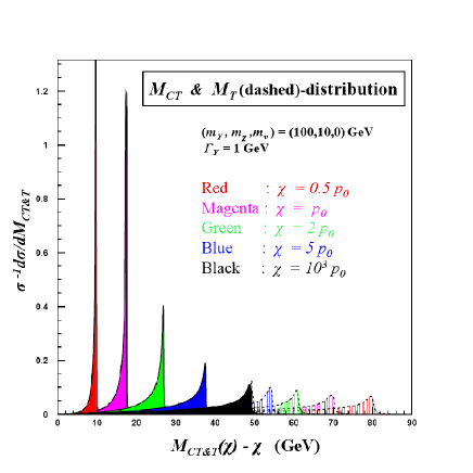
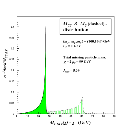
Fig. 1 shows the distribution of and when is transversely at rest in the lab. frame with , , and . The total decay width of , , was assumed to be 1 and spin angular correlation effect was ignored. In Fig. 1(a), we used a trial missing particle mass corresponding to where is . The black dashed line filled with green hatch corresponds to distribution and the black line is distribution. As explained, and share the same minimum at , but the endpoint of shrinks into a lower region so that the expected endpoint is while , ignoring the width effect. The height of the peak in distribution is amplified by the factor compared to the peak of . Fig. 1(b) shows how and are varied with respect to the trial missing particle mass . As shown in the figure, when the is small, diverges(red: ), and distribution collapses into a narrow peak region. On the other hand, if is large, then and become the same (black: ).
Now we have a collider variable which can drastically change and magnify its endpoint structure compared to that of . Basically, they provide the same physical constraint. Nevertheless, there is a big difference on the systematic uncertainties at these two end point regions. So, we move on to discuss how the amplification of the endpoint structure accompanies the propagation of statistical and systematic uncertainties.
In principle, one can try to use the sharp amplified endpoint instead of the endpoint in order to measure the mass constraint more precisely. However, one must be sure about that a naive statistical uncertainty cannot be reduced since as decreases to , the error propagation factor for increase by . On the other hands, things change when it comes to the systematic uncertainties. Actually, the endpoint structures we want to resolve are not that simple. If we attempt an accurate mass(endpoint) measurement with exact distribution shapes or templates, one have to understand the important dynamics of the new signal and backgrounds(surely also with the good understanding of the detector responses), which must include large systematic uncertainties. In this regard, model independent mass(endpoint) measurement will be important.
An effective way to measure the endpoint is simply observing and pinpointing the breakpoint(BP) with simplified local fit function up to some smearing width in the distribution. In this respect, it is important to know the effective range near the BP for the simplified local fit functions to be reliable, because we suffer from a large uncertainty in the bulk distribution. However, it is not apparent when the signal endpoint structure is dim and faint with feet or long tail above some irreducible backgrounds so that the BP is quite ambiguous with a small slope discontinuity. [We will assume that the background distribution is not singular at the BP.] When we attempt to identify a BP as the position of a meaningful endpoint, a slope discontinuity between the lower and the upper region of the BP is crucial factor for the BP measurement with less errors. The propagated uncertainty of the BP can be given as follows:
| (10) |
where is an error which can be caused by various sources, and is the slope difference between the two regions segmented by the BP. may come from event statistics or some systematic uncertainties. The point we note here is that the larger the slope difference, the clearer the endpoint structure, and as a result it enables us to elaborate the fit function and to choose more effective range of the fit function. In this regard, the elaboration of the fit scheme will reduce , and as a result will be reduced.
For the same reason an ambiguous faint endpoint in the distribution can be measured more precisely in the projection, and as a result the systematic error in obtaining the mass constraint , , can be reduced by . The specific estimation of error suppression factor is based on the following two facts,
-
(1)
The projection amplifies the slope difference near the endpoint by ,
(11) -
(2)
By the enhancement of the slope discontinuity, in the projection can be less than, or at least comparable to the case with refined fit scheme near the enhanced endpoint
(12)
Then , and if we take into account the error propagation factor for , we get .
Up to now we described that is well-defined variable using and trial missing particle mass in the rest frame of . The large amplification factor can be obtained simply by changing , and there is no additional parameter needed to accentuate the dim BP of the distribution. One might have a good chance to reduce some systematic uncertainty in extracting the mass constraints with the projection.
III constransverse mass,
In this section we introduce constransverse mass() for new physics events with two missing LNPs, which inherits the properties of . Some differences of using and will be discussed also.
When can we observe such an endpoint in a real experiment? One thing we should remind is that the maximum of and , and , are not invariant under the mother particle’s transverse motion when is not true value. One more shortcoming for is that it is not also invariant under the transverse boost of the mother particle, even when is true value. The reason for this is simply that in (3) is not an invariant quantity under the boost of mother particle, while (the endpoint value of ) is an invariant one, as has been utilized to measure the W-boson mass provided with already known neutrino mass mt ; mtmt2exp . However if we assume that we do not know the mass of the missing LNP, , while we just want to measure some mass constraints related to the decay process, then has no disadvantages compared to . As we will see in the examples of the following section, it can be much better to use or for this purpose. Then, it is just required for us to choose our decay system of interest being at rest in the transverse direction.
When the mother particle is boosted in the transverse direction with momentum, , the shift of the endpoint is described by
where , , , and is the azimuthal angle of visible particle in the mother particle’s rest frame. The shift is of order in general, and one should take care of the use of the endpoint for the mother particle with sizable transverse momentum in the lab. frame. cut must be accompanied with a proper event selection. Surely, the suppression cut might reduce the statistics of the signal event candidates. However, the cut can also play a role for purifying the signatures from backgrounds in many cases. We will describe such an effect of the cut with a new physics example, using endpoint in the next section.
Then, let us consider the production of a pair of identical new physics particles at the LHC, in which each of two mother particles decays to visible and invisible particles , (). Here with its transverse momentum() denotes the other particles not from the decays, so that it provides the transverse momenta of system as . In this case, we find that it is also possible to observe the same -like endpoint by the construction of constransverse mass, by
| (13) | |||||
where is a trial missing particle mass, and . Here all the particle momenta are defined in the lab. frame. is the contransverse mass of each mother particle system as defined in (3) using a trial transverse momenta which satisfies the missing transverse momentum condition. This is the contra version of Cambridge stransverse mass () variable mttwo . Please note that in (13) is defined for the mother particle pair where each mother particle can have sizable transverse momentum in the lab. frame, and it can make shifted as explained previously. However, an interesting point is that if , system is transversely at rest, and the also has well-defined endpoint as in (7). This is analogous to the case that becomes when the mother particle has no transverse momentum. To be analytically exact for that result, let us see the solution of . If , the analytic solution is given as follows,
| (14) | |||||
ignoring the mass of the visible particles.333In the rest of this paper, we concentrate on the events with one massless visible particle in each decay chain. The solution can be obtained just by using the visible momenta with the sign flip in solving the balanced equation as in Refs. mt2kink ; mtgen . From (14), one can see that as the natural extension of ,
| (15) |
in the limit of . This can be easily proved from Eq. (14), assuming the situation where the two mother particles are at rest in the lab. frame and all the relic particles are in the transverse plane. Such a pair of rest mother particles can be guaranteed by the back-to-back boost invariance of solution (14). It is interesting to note that is described by the value in general, in spite of the nonzero transverse momentum for each of the mother particles. This is the same phenomenon that inherits most of the important properties of , so that also. Physically Eq. (15) can be satisfied by the events with kinematically identical decay chains, each of which has the maximal or configuration. So in this case, (or ) can be effectively the same as the single (or ). This is also true for the event contributing to the minimum.
The other important inheritance of from is that the Jacobian factor in (9) should be valid also between the and , at least for the maximum and minimum regions of both variables as explained. In the maximum region, the and solutions are perfectly described by in (15) and in (8), respectively, while in the minimum region, both and become the same value, giving the Jacobian factor of .
Fig. 2 shows how the previous analysis of and is extended to the and analysis for the SUSY(sps1a) event when a pair of right handed squarks() are produced, and each decays to a quark and an LSP(),(). It is a parton level simulation with no initial state radiation(ISR) effect so that .
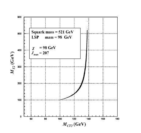
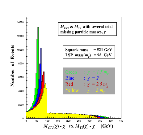
Fig. 2(a) is a scatter plot of the events in the - plane for . As expected from the previous and analysis, most of the large events are projected into a narrow endpoint region of the variable, reflecting the large factor for the endpoint region of distribution. Fig. 2(b) is a comparison plot between the and distributions for [green], [blue], [red], and [yellow]. The uprisen distributions are and the laid distributions are . For , the endpoint enhancement factors, of (9), are estimated to be , , , and . As in Fig. 1, we can also observe a similar behavior such that if is small then the distribution collapses into a region near zero with a diverging , while it approaches to when has a large value.
As a result of a large factor, a small slope difference in the distribution can be amplified also in the projection by a factor of , naturally transformed into a remarkably enhanced or uprisen endpoint structure of the mother particles. Therefore, as discussed in the previous section, the projection also can help us to extract a meaningful endpoint defined as a BP in the distribution. Even though there exist heavy systematic uncertainties in the signal and backgrounds, the dim BPs will be amplified and it can significantly reduce the systematic uncertainties we suffered from in fitting with more elaborated fitting schemes. Fig. 3 shows the (uprisen) and (laid) distributions of slepton pair production events, where a pair of right(left) handed sleptons( GeV) are produced(sps5), and each slepton decays to with GeV.

This is also a parton level result and we used . In the distribution, there exists a BP which is made by the endpoint of but buried in the signature. One can see that such a BP is enhanced in the projection, where the factor for is 5.3 for . With this example, one might naturally think about the possibility to resolve some mass hierarchies with reduced systematic uncertainties using the projection of some inclusive event data. The mass hierarchies will be represented by several values, for instance, here there are two values to be resolved as follows
| (16) |
each of which can be extracted from the first and the 2nd endpoints of the or distributions, respectively.
As we will see in the next section, projection can be a very powerful tool for resolving several values originated from various mass hierarchies between new particles. Basically, wherever there exist symmetric decay chains with various mass hierarchies, one can try to resolve them in terms of various values. If the symmetric chain involves three body decays like ()), the effective value which contributes to the endpoint of or will be . (Here the and is also defined with only 2 visible particles with properly modified missing .) From now on, we define by
| (17) |
Therefore, the projection enables us to implement some precision endpoint measurement using the inclusive signal and background data with large uncertainties. The amplification of some BPs by projection increases our observability for meaningful signal endpoints in distribution, which are buried in severe backgrounds.
IV Applications
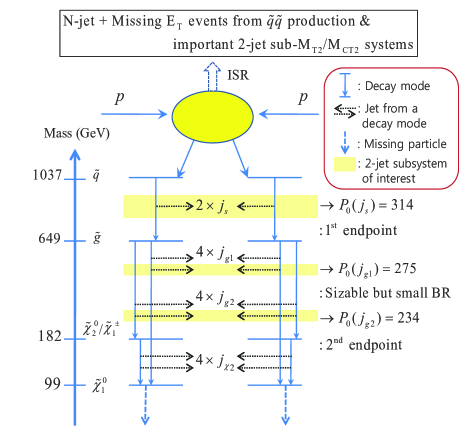
In this section, we will describe more useful example of projection in order to obtain some constraints between , , and other superparticle masses in a situation where large uncertainties are involved with jets. Specifically, an example of measuring some superparticle mass constraints via projection is shown, using 6 hard jets + signal from a SUSY model. The mSUGRA type SUSY benchmark spectrum is chosen in Table 1.
At this benchmark point, squark and slepton masses are heavier than gluino by a few hundreds . Also the 2nd neutralino and chargino are mostly wino so that their masses are nearly degenerate. Thus, if we take into account the production and decay rates at the LHC energy of 14 TeV, the important new particle mass hierarchies can be categorized by 4 mass scales listed in Table 1. and productions are the dominant superparticle generation processes with for both cases. production also has a sizable cross section about . Lepton production is suppressed here because sleptons are also very heavy so that leptons cannot be generated via some cascade decay chain of gluino or squarks. So most of new physics signals are hard N-jets + signal from squark or gluino decays. Several important squark and gluino decay chains give the following branching ratios
-
1.
-
2.
-
3.
-
4.
Here, all the listed gluino branching ratios are for 3 body decay processes via virtual squarks. The inclusive hard N() jets + signal can come from heavy squark pair production where each squark decays to , and subsequently, through 3 body decay chain,
| (18) |
where is the extra particles(e.g. ISR) which gives a recoil transverse momentum to the system. Fig. 4 shows the event topology of the production we consider. and in (18) denote the jets from squark decay and gluino decay, respectively. can be separated to and as in Fig. 4, according to their decay processes. In this paper, and are assumed to decay to light jets() + via or bosons if they are produced in the gluino decay.
In this regard, phenomenologically the most important question would be, “How can we measure the superparticle masses using N-jets + signal in a situation with large jet uncertainties in identifying true signal jets with complex combinatorics?” One might attempt to measure the gluino or squark masses using the so-called ‘-kink method mt2kink ’. According to this method, one can have a good chance to measure the squark(or gluino) and masses simultaniously by extracting the position of the kink, if 6 jets(or 4 jets) from squark(or gluino) pair decays are efficiently identified. In particular, for gluino mass measurement, if squarks are very heavy so that they are decoupled at the LHC, then most of the hardest 4 jets would be from the decays from the gluino pair, the efficiency of choosing the correct 4 jets can be quite nice. However, when squarks are heavier than gluino by just a few hundred , then the efficiency gets worse, particulary for when () is comparable to, or larger than (). Although the squark pair production rate decreases as the () increases, the two with hard are more likely to be selected in the gluino calculation, and badly pollute the endpoint structure mt2kinkinclusive . Furthermore, the ISR can be an important source of jet backgrounds with hard also mt2kinkisr ; qcdisr . Thus, there exists a large amount of systematic uncertainty in correctly estimating the jet backgrounds of gluino .
As we will describe soon, the projection can help resolving several mass differences hidden in various inclusive jet signatures in general. The mass differences are represented by several values in the endpoints measurements of the and distributions, as we discussed in the previous sections. Such values are listed in Fig. 4, whose values have been calculated by (17).
Here we concentrate on measuring the mass difference between squark and gluino since the usual gluino mass measurements have a lot of uncertainties as we explained in the previous paragraph. After the description of this specific example, we will present a generalization of the amplification for resolving several mass hierarchies which have been buried in various inclusive signatures, so regarded as meaningless in the distribution.
Our strategy for measuring the squark-gluino mass difference is naturally focusing on the two rather than trying to select four from gluino pair decays. Surely, there exists a large amount of uncertainty in correctly choosing two and estimating the backgrounds also. However, we attempted to calculate and for the Subsystem (), considering two gluinos as the effective missing particles for the system. Once we could construct the Subsystem- (M. Burns et. al. in mt2ext ) using the correct pair of two , then in the limit of vanishing , its endpoint corresponds to in (8) with given by
| (19) |
| 12.2 | 0.01 | 0.12 | |||||
| 3.9 | 0.03 | 0.11 |
Therefore, the measurement of the Subsystem- endpoint
can provide us a constraint between and .
Once we assume that the and masses could be
already obtained through the -kink methods using 6 hardest
jets, then might be also measured by
(19). However, as commented previously, the endpoint
measurement of the Subsystem- distribution is not easy.
Choosing the correct pair of two suffers from the jet
uncertainties, and hence some effective event selection cuts or methods
purifying the signals should be applied. Thus, we describe another
approach to the endpoint measurement of the Subsystem-.
In short, it can be summarized as follows :
We do not care whatever backgrounds there exist. Once
there is a dim BP from a signal endpoint in the
distribution with large systematic uncertainties, then we can try to
extract the position of the amplified BP in the projection.
With this point of view, we calculate the Subsystem- and Subsystem- variables for all possible 15 pairs of the two jets among the 6 highest jets in an event with N()-jets + . If the event is from a real squark pair production, then there exists at least one true pair of two among the 15 pairs of possible two jets, and it might consistently contribute to the meaningful endpoint in the Subsystem- distribution, although the slope change must be faint. The portion of true two pair will be much more reduced if we take into account the background events, e.g. , + etc with hard ISR effects. Anyway, using the events with N()-jets + , we tested the possibility to measure the corresponding amplified BP in the projection with less systematic errors. Extracting meaningful endpoints using more inclusive events with general N()-jets + will be discussed in the latter part of this section and a forthcoming paper nextmct2 . We found that even with this small fraction of N()-jets + events, a sizable number of events survive the usual new physics cuts, and contribute to some meaningful amplified BPs of the inclusive Subsystem(IS)-. To reconstruct the BPs in the IS- and , the 15 values of Subsystem- and Subsystem- are constructed with given trial gluino masses for an event as follows and we made histograms of all the calculated values without any preferential jet selection among the 6 hardest jets,
| (20) | |||||
The index means a specific combination to select
two among the 6 hardest jets. are
the transverse momenta of the two jets selected as in the lab.
frame. is the total missing transverse momenta, and
is modified missing transverse momenta for the
subsystem with indicating the sum of
the remaining 4 jets which are selected as four in the -th
combination. is meant to be a trial gluino mass with this
setup of visible and missing momenta.
We simulated the production events of at the LHC energy of 14 TeV using PYTHIA 6.4 pythia with ISR/FSR turned on. Fully showered and hadronized events were passed to the PGS 4.0 detector simulator pgs . The energy resolution parameter in the hadronic calorimeter was given by , and jets were defined using a cone algorithm with . To be more reliable for the new physics event experiments, we imposed several cuts for pure N-jets + events atlas ; cms ; alpha although we did not include the SM background event samples for simplicity.
The event selection cuts were as follows:
-
1.
No leptons, no jets in the event,
-
2.
Number of jets with ,
-
3.
,
-
4.
with for the pairs
of selected two jets, -
5.
,
where the index- denotes the 6 hardest jets. The alpha where and are the of the second hardest jet and dijet invariant mass, respectively, for the -th pair of selected two jets. If decay directly to , then becomes which is the total transverse momentum of the squark pair system defined in (18). As explained in the previous section, the fifth cut is imposed to suppress the shift of the endpoint (15) under arbitrary transverse boost of two mother particle system().444The endpoint with a sizable will be studied in a forthcoming paper nextmct2 . We calculated the and for all the events passing the cuts. The single jet invariant masses, in calculating the and of (20) was ignored since we found that it is quite helpful for the endpoints of both variables to be located at the expected position, reducing the jet energy resolution effect. Ignoring the jet masses also satisfies all the inequalities of and and the constructed variables can saturate to the boundary value because of enough statistics of light QCD jets in the events. In our SUSY event sample, the jet multiplicity ratio is . With the relatively small portion of the event sample () surviving the cuts, we still could observe the BP in the IS-, and the amplified BP in the IS- also.
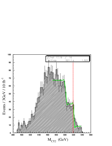
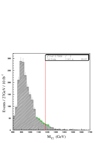
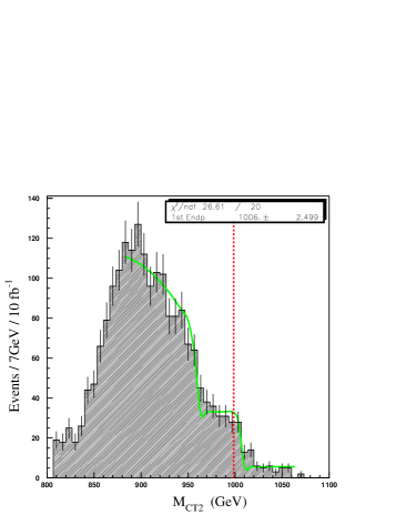
Fig. 5(a,b)(two histograms in the top) shows the and the corresponding distributions for GeV. Fig. 5(c,d)(two histograms in the bottom) are also and for GeV. The endpoint enhancement factor, is 12.2 for (a)(b), and 3.9 for (c)(d). We constructed many histograms with respect to various values. Among them, we selected the two cases as shown in Fig. 5. Actually, compared to , a much larger or smaller value of is not a good choice as explained in the previous section. Based on our trial experience, choosing of order of shows a proper amplification feature with clean breakpoint structures, and this selection can be realized by observing an average value of of the hardest jets. A strong -suppression cut was quite effective for observing a BP with a small slope discontinuity at the expected endpoints in the distributions, and we could observe the amplified BPs also at the expected position in the corresponding distributions. Actually, this cut is effective for selecting the production event. The expected endpoints are pinpointed by a red dashed line in each figure. The bin interval was selected as the best one among several bin candidates, by which the histogram near the expected BP regions shows its characteristic feature maximally while keeping its statistical relevance.
In Fig. 5(a), the distribution shows a small slope discontinuity near the expected endpoint . One can find that the faint BP structure is amplified near the expected endpoint in the (Fig. 5(b)) projection, producing a sharp cliff wall. Similarly, there exists a small BP near the expected endpoint GeV of distribution in Fig.5(c), and the BP is transformed to another BP with a sharp cliff near the expected endpoint of in Fig. 5(d).
Table 2 shows the expected and fitted endpoints of the and distributions for and . The errors after the fitting process are also listed in the columns of and . Here, the first error represents statistical one, and the second represents the systematic one in the fitting process. The fit model functions for the endpoints were a Gaussian smeared linear function for a signal, and a linear function for the backgrounds in the distributions (Fig. 5(a,c)),
| (21) | |||||
Also, the endpoint region of the distribution (Fig. 5(b,d)) was fitted by the Gaussian smeared step functions for signals, and step function for backgrounds,
| (22) | |||||
Fitting was implemented by the binned method using MINUIT with MINOS error processing minuit which takes into account both parameter correlations and non-linearities. The two step functions for signal endpoints was designed in (22) to fit two cliffs appearing in the distributions. We will explain the second endpoint below the 1st endpoint which were pointed by red dashed line in the distribution (Fig. 5(b,d)) in the latter part of this Section. For simplicity, we used the same smearing widths for both the two endpoint cliffs in the distribution. Actually, the uncertainty from the endpoint broadening effect by some widths is not our issue here. As described in Sec. II, it is simply because the endpoint uncertainty reduction factor is expected to be just the order of in that case, and the reduced width is compensated by the explicit error propagation factor for obtaining value. It is natural that there is no advantage in using projection for reducing the statistical errors. Anyway, the fitted endpoint values were found not to be very sensitive to the choice of in the range GeV for , and 0–1 GeV for , and we fixed the smearing widths to be 5 GeV for the endpoint, and 0.5 GeV for the endpoints. The width for the endpoint is a suppressed value from the width of the endpoint by .
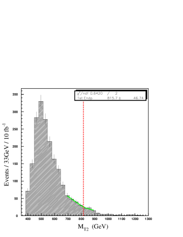
, , , .
The green lines in Fig. 5 represent the fitted model function. In order to estimate the systematic uncertainty, we attempted to fit various endpoint regions with the simple model functions while keeping the after fitting( = the number of fitted bins – 1). The small value of might guarantees the plausibility of the fit range described by the model function. Actually, for anyone trying to find some optimal range of the fitting in the distribution, he easily notices that there exist a large number of choices for a lower boundary and an upper boundary, which is consistent with small after fitting. In this situation, because the BP is quite a faint one can observe that the fitted endpoint parameter changes very much with a large uncertainty as the fit range of validity is varied. On the other hand, the fitting of the endpoint regions can be different. Due to the emergence of the sharp cliffs, which are the amplified BPs, we could clearly elaborate our effective fit model functions and the fit ranges of validity. Actually, there is another meaningful BP near GeV in the distribution, which is now clearly seen as the cliff near GeV in the projection(For , a similar BP enhancement is observed). It looks even more clearer than the first BP we expected for the squark pair decays. In the past, one would have neglected such a BP buried in the region of the low distribution, as well as suffer from large systematic uncertainties in extracting the position of the first BP. Now, in addition to the first endpoint(red dashed), we can try to extract the amplified second lower endpoint and interpret its origin with less uncertainty.
One can easily see that the second endpoint is originating from the mass differences between the and , represented by another value,
| (23) |
This is the maximal momentum of jets from a gluino three body decays to in the rest frame of the gluino. Since the BR() is times larger than the BR(), gluino decays to can contribute significantly to the inclusive N()-jets + signature than the gluino decays to since most of the hadronically decays to 2-jets() + via bosons. The point we want to emphasize here is that, once there is some possibility of a pair of mother particles to be symmetric in the lab. frame(), then as analyzed in Sec. II, it might contribute to some other endpoint in the distribution with some value defined in (17). For example, in the squark pair production events we consider, the symmetric condition of a pair of gluinos can be realized if
| (24) |
However, regardless of the gluino pair symmetry condition, and in (20) can include Subsystem- and for the subsystem which consist of two visible + effective , if the two in (20) correspond to the transverse momenta of two . Here means the 2 gluino jets , each of which comes from each mother gluino, and is selected for . The corresponding subsystem is described in the third yellow box of Fig. 4. If denotes the other two which are not selected as the subsystem visible particles, then the effective missing transverse momenta, in the (20), and in the event selection cuts become as follows:
| (25) | |||||
| (26) | |||||
where the assumption that is not included in the 6 hardest jet candidates is adopted. Then, our strong suppression cut implies that the effective missing transverse momenta are
| (27) |
This indicates that Subsystem- and in (20) can have a good chance of contributing to the well-defined endpoints described by value if the gluino symmetric condition (24) is satisfied. In that case, the contribution consistently forms the slight slope change in the distribution, and it will emerge as a sharp cliff in the distribution. In our example, the strong suppression cuts of (26) effectively acts as a suppression cut, and then it will create a bias to choose small events because distribution is expected to be an even convex function when is zero. Then, the symmetric condition can be effectively satisfied for a lot of events, and there exist large contributions to form some slope change near the expected exact second endpoint.
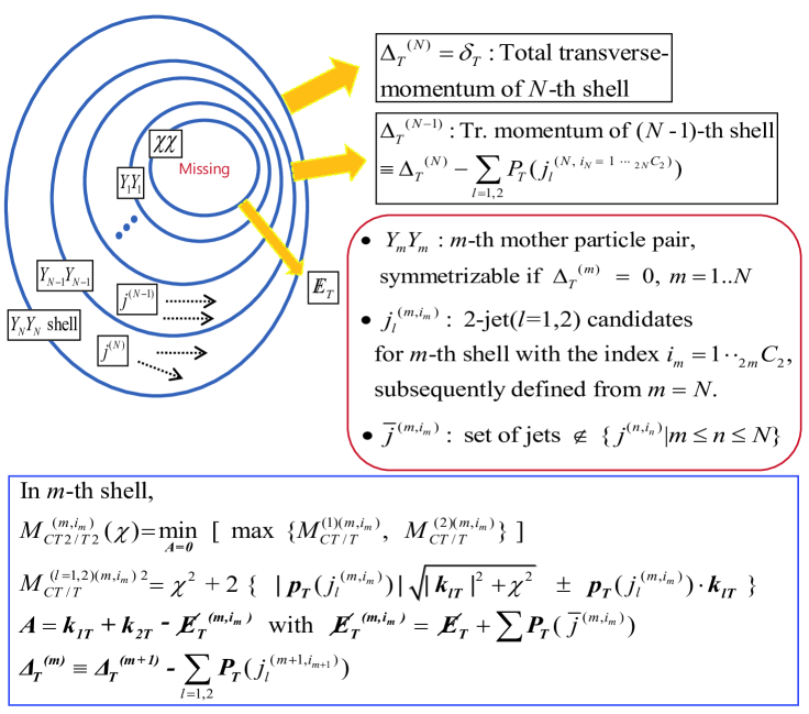
However, one can easily notice that the suppression cut cannot guarantee the exact symmetric condition of the gluino pair. In order to access to each symmetric mother particle pairs possibly hidden in the N-decay shells, one can extend the definitions of Subsystem- and of (20) as shown in Fig. 6. Here, with hard ()-jet + inclusive signatures, one can subsequently construct all the possible -th Subsystem-, variables from the highest shell, which has a well-defined generalized symmetric condition parameter, . In general, Subsystem- and have (=) multiplicity which is the number of jet combinations possible in the -th shell. As a result one can explicitly control those cut parameters to observe the amplified BPs from several symmetrized mother particle pairs. Furthermore, one can find that to realize the hidden endpoints the one-dimensional decomposed version decompose of Subsystem- and , and , can be useful, if it is constructed using only partial components of perpendicular to direction. In this regard, a more general spectroscopy will be discussed in a forthcoming paper nextmct2 . As a result several mass hierarchies in various new physics models can be probed by general Subsystem- amplification using the inclusive N()-jets/leptons/photons + signatures, with less systematic uncertainties.
Finally, we summarize the fit results of the first endpoints(red dashed) in the column, and , of Table 2. Using dozens of fit results for various fit ranges, we evaluated the statistical errors as GeV for , and 1.6 GeV for . The listed systematic uncertainties were obtained by from the fitted endpoint values. It is noticeable that the systematic errors are suppressed in the by the factor of for or less than that for , while all of the statistical errors are reduced by the order of . As a result, the precision to measure the can be enhanced at least by a factor of as listed in the last column of Table 2. These results are well matched with our expectation of the endpoint structure enhancement by the projections.
Including more various systematic error effects (the SM backgrounds, the signal and BGs in higher orders, PDF) is beyond the scope of this paper. But, the main point of this paper is clear: The features of the BP enhancement by projection has a more stronger power in resolving the buried mass hierarchies as our situation gets worse with large uncertainties.
V Conclusion
We have introduced the constransverse mass, , and have
shown that it can significantly increase our ability to measure
the endpoints precisely by amplifying the small slope discontinuity of the endpoint region, which are usually buried in the complex backgrounds
with large uncertainties. As a result, the proposed variable
for various subsystems with two visible particles can resolve the mass
hierarchies hidden in various inclusive signatures for the event
type, N()-jets/leptons/photons + . We hope
that this variable can be a useful tool in the LHC era.
Acknowledgements.
WSC thanks Kiwoon Choi for useful discussions, and Mihoko Nojiri for inviting him to the IPMU Workshop where this topic has been presented. WSC and JEK are supported in part by the Korea Research Foundation, Grant No. KRF-2005-084-C00001, and JHK is supported in part by Grant No. KRF-2008-313-C00162 and the FPRD of the BK21 program.References
- (1)
- (2)
- (3) ATLAS Technical Proposal, CERN-LHCC-94-43.
- (4) CMS Physics Technical Design Report, CERN-LHCC-2006-021.
- (5) H. P. Nilles, Phys. Rep. 110, 1 (1984); H. E. Haber and G. L. Kane, Phys. Rep. 117, 75 (1985).
- (6) N. Arkani-Hamed, A. G. Cohen and H. Georgi, Phys. Lett. B 513, 232 (2001) [hep-ph/0105239]; H. C. Cheng and I. Low, J. High Energy Phys. 09, 051 (2003) [hep-ph/0308199].
- (7) T. Appelquist, H. C. Cheng and B. A. Dobrescu, Phys. Rev. D 64, 035002 (2001) [hep-ph/0012100].
- (8) M. M. Nojiri, G. Polesello and D. R. Tovey, [hep-ph/0312317]; K. Kawagoe, M. M. Nojiri and G. Polesello, Phys. Rev. D 71, 035008 (2005) [hep-ph/0410160]; M. M. Nojiri, G. Polesello and D. R. Tovey, J. High Energy Phys. 12, 014 (2008) [arXiv:0712.2718] H. C. Cheng, D. Engelhardt, J. F. Gunion, Z. Han and B. McElrath, Phys. Rev. Lett. 100, 252001 (2008) [arXiv:0802.4290]; H. C. Cheng, J. F. Gunion, Z. Han, G. Marandella and B. McElrath, J. High Energy Phys. 12, 076 (2007) [arXiv:0707.0030]; H. C. Cheng, J. F. Gunion, Z. Han and B. McElrath, Phys. Rev. D 80, 035020 (2009) [arXiv:0905.1344]; B. Webber J. High Energy Phys. 09, 124 (2009) [arXiv:0907.5307]; C. Autermann, B. Mura, C. Sander, H. Schettler and P. Schleper, [arXiv:0911.2607];
- (9) I. Hinchliffe, F. E. Paige, M. D. Shapiro, J. Soderqvist and W. Yao, Phys. Rev. D 55, 5520 (1997) [hep-ph/9610544]; H. Bachacou, I. Hinchliffe and F. E. Paige, Phys. Rev. D 62, 015009 (2000) [hep-ph/9907518]; I. Hinchliffe and F. E. Paige, Phys. Rev. D 61, 095011 (2000) [hep-ph/9907519]; B. C. Allanach, C. G. Lester, M. A. Parker and B. R. Webber, J. High Energy Phys. 09, 004 (2000) [hep-ph/0007009]; B. K. Gjelsten, D. J. Miller and P. Osland, J. High Energy Phys. 12, 003 (2003) [hep-ph/0410303]; B. K. Gjelsten, D. J. Miller and P. Osland, J. High Energy Phys. 06, 015 (2005) [hep-ph/0510033]; D. Costanzo and D. R. Tovey, J. High Energy Phys. 04, 084 (2009) [arXiv:0902.2331]; M. Burns, K. T. Matchev and M. Park, J. High Energy Phys. 05, 094 (2009) [arXiv:0903.4371]; K. T. Matchev, F. Moortgat, L. Pape and M. Park, J. High Energy Phys. 08, 104 (2009) [arXiv:0906.2417]; M. Bisset, R. Lu and N. Kersting, [arXiv:0806.2492]; N. Kersting, Euro. Phys. J. 63, 23-32 (2009) [arXiv:0806.4238]; N. Kersting, Phys. Rev. D 79, 095018 (2009) [arXiv:0901.2765]
- (10) V.D. Barger, A.D. Martin and R.J.N. Phillips, Z. Phys. C 21 (1983) 99; J. Smith, W. L. van Neerven and J. A. M Vermaseren, Phys. Rev. Lett. 50, 22 (1983)
- (11) T. Aaltonen et al. (CDF Collaboration), Phys. Rev. D 77, 112001 (2008) [arXiv:0708.3642]; T. Aaltonen et al. (CDF Collaboration), [arXiv:0911.2956]; W. S. Cho, K. Choi, Y. G. Kim and C. B. Park, Phys. Rev. D 78, 034019 (2008) [arXiv:0804.2185]; A. Barr, B. Gripaios and C. G. Lester, J. High Energy Phys. 07, 072 (2009) [arXiv:0902.4864]
- (12) C. G. Lester and D. J. Summers, Phys. Lett. B 463, 99 (1999) [hep-ph/9906349]; A. Barr, C. G. Lester and P. Stephens, J. Phys. G29 (2003) 2343 [hep-ph/0304226].
- (13) W. S. Cho, K. Choi, Y. G. Kim and C. B. Park, Phys. Rev. Lett. 100, 171801 (2008) [arXiv:0709.0288]; B. Gripaios, J. High Energy Phys. 02, 053 (2008) [arXiv:0709.2740]; A. J. Barr, B. Gripaios and C. G. Lester, J. High Energy Phys. 02, 014 (2008) [arXiv:0711.4008]; W. S. Cho, K. Choi, Y. G. Kim and C. B. Park, J. High Energy Phys. 02, 035 (2008) [arXiv:0711.4526].
- (14) M. M. Nojiri, Y. Shimizu, S. Okada and K. Kawagoe, J. High Energy Phys. 06, 035 (2008) [arXiv:0802.2412]; M. M. Nojiri, K. Sakurai, Y. Shimizu and M. Takeuchi, J. High Energy Phys. 06, 100 (2008) [arXiv:0808.1094]
- (15) J. Alwall, K. Hiramastsu, M. M. Nojiri and Y. Shimizu, Phys. Rev. Lett. 103, 151802 (2009) [arXiv:0905.1201]
- (16) M. Burns, K. Kong, K. T. Matchev and M. Park, J. High Energy Phys. 03, 143 (2009) [arXiv:0810.5576]; K. T. Matchev, F. Moortgat, L. Page and M. Park, [arXiv:0909.4300]; P. Konar, K. Kong, K. T. Matchev and M. Park, [arXiv:0911.4126]
- (17) R. Tovey, J. High Energy Phys. 04, 034 (2008) [arXiv:0802.2879]; M. Serna, J. High Energy Phys. 06, 004 (2008) [arXiv:0804.3344]; G. Polesello and D. R. Tovey, [arXiv:0910.0174]
- (18) T. Han, I.W. Kim and J. Song, [arXiv:0906.5009]; I. W. Kim [arXiv:0910.1149]
- (19) D. J. Miller, P. Osland and A. R. Raklev, J. High Energy Phys. 03, 034 (2006) [hep-ph/0510356]; C. G. Lester, Phys. Lett. B 655, 39 (2007) [hep-ph/0603171].
- (20) G. G. Ross and M. Serna, Phys. Lett. B 665, 212-218 (2008) [arXiv:0712.0943]; M. Serna, J. High Energy Phys. 06, 004 (2008)[arXiv:0804.3344]; A. J. Barr, G. G. Ross and M. Serna, Phys. Rev. D 78, 056006 (2008) [arXiv:0806.3224]; A. J. Barr, A. Pinder and M. Serna, Phys. Rev. D 79, 074005 (2009) [arXiv:0811.2138]
- (21) H. C. Cheng and Z. Han, J. High Energy Phys. 12, 063 (2008) [arXiv:0810.5178]; A. J. Barr, B. Gripaios and C. G. Lester, J. High Energy Phys. 11, 096 (2009) [arXiv:0908.3779]
- (22) C. G. Lester and A. J. Barr, J. High Energy Phys. 12, 102 (2007) [arXiv:0708.1028]
- (23) P. Konar, K. Kong and K. T. Matchev, J. High Energy Phys. 03, 085 (2009) [arXiv:0812.1042]
- (24) W. S. Cho, K. Choi, Y. G. Kim and C. B. Park, Phys. Rev. D 79, 031701 (2009) [arXiv:0810.4853]; K. Choi, S. Choi, J. S. Lee and C. B. Park, Phys. Rev. D 80, 073010 (2009) [arXiv:0908.0079]; N. Kersting, Phys. Rev. D 79, 095018 (2009) [arXiv:0901.2765]; Z. Kang, N. Kersting, S. Kraml and A. R. Raklev, [arXiv:0908.1550]
- (25) J. Alwall, S. Visscher and F. Maltoni J. High Energy Phys. 02, 017 (2009) [arXiv:0810.5350]; A. Papaefstathiou and B. Webber, J. High Energy Phys. 06, 069 (2009),[arXiv:0903.2013]
- (26) K. T. Matchev and M. Park, [arXiv:0910.1584]; P. Konar, K. Kong, K. T. Matchev and M. Park, [arXiv:0910.3679]
- (27) W. S. Cho, work in progress
- (28) PYTHIA, T. Sjostrand, S. Mrenna and P. Skands, LU TP 06-13, FERMILAB-PUB-06-052-CD-T [hep-ph/0603175]; T. Sjostrand, S. Mrenna and P. Skands, Comput. Phys. Commu. 178, 852-869 (2008) [arXiv:0701.3820]
- (29) SOFTSUSY, B. C. Allanach, Comput. Phys. Commun. 143, 305-331 (2002) [arXiv/0104145]
-
(30)
PGS 4, http://www.physics.ucdavis.edu/conway
/research /software/pgs/pgs4-general.htm. - (31) L. Randall and D. Tucker-Smith Phys. Rev. Lett. 101, 221803 (2008) [arXiv:0806.1049]
-
(32)
MINUIT, CERN program library long writeup, D506.
http://seal.web.cern.ch/seal/snapshot/work-packages/mathlibs/minuit/