Fitting and Comparison of Models of Radio Spectra–Publication information;
Fitting and Comparison of Models of Radio Spectra
Abstract
I describe an approach to fitting and comparison of radio spectra based on Bayesian analysis and realised using a new implementation of the nested sampling algorithm. Such an approach improves on the commonly used maximum-likelihood fitting of radio spectra by allowing objective model selection, calculation of the full probability distributions of the model parameters and provides a natural mechanism for including information other than the measured spectra through priors. In this paper I cover the theoretical background, the algorithms used and the implementation details of the computer code. I also briefly illustrate the method with some previously published data for three near-by galaxies. In forthcoming papers we will present the results of applying this analysis larger data sets, including some new observations, and the physical conclusions that can be made. The computer code as well as the overall approach described here may also be useful for analysis of other multi-chromatic broad-band observations and possibly also photometric redshift estimation. All of the code is publicly available, licensed under the GNU General Public License, at http://www.mrao.cam.ac.uk/~bn204/galevol/speca/index.html.
1 Introduction
The spectrum of radio emission from the majority of astronomical sources consists of a smooth continuum with (in some but not all sources) atomic and molecular lines superimposed, most notably the H i line at 1.42 GHz and the carbon monoxide rotational line ladder starting at 115 GHz. Measurements with significant fractional bandwidths are almost always dominated by the continuum emission.
The shape of the continuum emission can be measured by making observations at widely spaced frequencies. The available measurements for some local objects span a very wide range of frequencies, from about 50 MHz to above 1 THz and into the far-infrared portion of the spectrum. The measured shape of the continuum emission naturally provides information about the physical properties of the sources and mechanisms for emission. There are many examples of physical properties which one can try to extract:
-
•
The slope of the synchrotron emission gives the energy spectrum of relativistic electrons in the source, providing constraints on the mechanism by which they are created
-
•
The change in slope in the synchrotron spectrum gives an estimate of the age of the source
-
•
The low frequency turn-over, i.e., where source becomes opaque due to absorption due to electrons, places constraints on the geometry of the source
-
•
The slope of the Raleigh-Jeans part of the dust spectrum places constraints on the properties of the dust
-
•
The frequency of the peak of the dust spectrum determines the temperature of the dust and the total power output of the source
Additionally one can try to make an estimate of redshift of a distant object from the observed spectral shape.
Most of the physics underlying the emission processes at these wavelengths is well understood and it is possible to calculate the expected spectrum given a model and its parameters. Therefore, analysis of radio continuum spectra often consists of ‘fitting’ a selection of known models to the observations.
Some of the desirable outputs of such an analysis are:
-
1.
An objective measure of how well the model explains the data
-
2.
Unbiased estimates of parameters of the model, estimates of errors with which these estimates are made, and the correlations between the estimate errors
-
3.
Full probability distributions of parameters in cases that they are significantly non-Gaussian
-
4.
An objective way of comparing how well different models explain the same data
All of these can be obtained simultaneously using Bayesian analysis and the nested sampling algorithm. In this paper I describe a computer code to perform this analysis and illustrate it with examples using previously published data for three near-by galaxies.
This code was developed to support an ongoing observational programme to measure the radio spectral energy distributions of near-by star-forming galaxies. We are also currently applying he code to analyse the spectra of Ultra-Luminous InfraRed Galaxies (ULIRGs) with the goal of better understanding the their radio emission and the physical conditions within them. These results will be published separately in forthcoming papers.
2 Method
The analysis proceeds in the usual fashion, starting with the Bayes equation (see for example: Jaynes 2003; Sivia & Skilling 2006):
| (1) |
where the symbols have following meaning:
-
is the hypothesis under which the data are analysed. In this case, the hypothesis consists of the model we assume for the radio emission and the priors for each of the model parameters
-
is a vector with elements that are the parameters of the model (e.g., the spectral index , the frequency of the spectral break )
-
are the observed data (in this case, the observed flux densities at various frequencies)
-
is the probability that the model parameters take a particular value, i.e., the prior information associated with the hypothesis that we are using
-
is the likelihood, i.e., the probability of observing the data we have given some model parameters
-
is the so-called Bayesian evidence, that is a measure of how well our hypothesis (i.e., the model for the emission spectrum and the priors) predict the data actually observed
-
is the posterior joint distribution of the model parameters
The two inputs to the calculation are:
The computation is done using the nested sampling algorithm (Skilling 2006) as described in Section 2.3.
The two outputs are:
-
1.
, the evidence for the model and the prior
-
2.
, the posterior distribution of the model parameters
2.1 Models of synchrotron radiation spectra
In general, the models that it makes sense to try when analysing a particular set of observations are determined by the type of object that has been observed and the region of the spectrum which is being analysed. The current version of the computer code described here already has implementations of models which combine absorption, synchrotron and thermal radiation.
In this paper however, I restrict the description to models of non-thermal synchrotron emission. The reason is that in the examples shown later I use only measurements below 5 GHz while the synchrotron mechanism is the dominant component of emission from the majority of extragalactic sources at frequencies below about 50 GHz, so this is a reasonable approximation. The remaining models present in the software implementation will be used for forthcoming science papers and they can easily be extended further still with thermal dust or spinning dust emission for example.
The simplest model of synchrotron emission spectrum is a simple power-law model:
| (2) |
with two parameters:
-
The flux density at the frequency of 1 GHz
-
The spectral index
It is not however convenient to make a parametrisation directly in terms of since it can take large range of values for typical sources, and we do not a-prior know even the order magnitude of to expect. For example, if we assumed that could be any value between 0.01 and 1 Jy with uniform probability then there would be far more values with magnitude of order of 1 than of order 0.01. Instead, I parametrise the model in terms of the logarithm of , i.e., and assume that this is uniformly distributed over a range of values (-2 to 0 in the example above). There is further discussion of this topic of so-called scale parameters by Jaynes (2003).
A more complicated and physically more accurate model is the so called continuous-injection model (e.g., Kardashev 1962). In this model it is assumed that the energetic electrons have a power-law energy distribution when they are created, and that these freshly-created electrons are continuously added to the plasma at a constant rate. As the electrons emit synchrotron radiation they naturally loose energy. The rate of energy losses is however higher for the higher-energy electrons, and this leads to a ‘break’ in the emission spectrum of the plasma. The resulting spectrum can be approximately described by:
| (5) |
The one new parameter in this model is the frequency of break in the spectrum, . If this break frequency is known, it can be used to estimate the age of the source given the magnetic field strength within it and vice-versa.
Like the flux density scaling parameter , the frequency of the spectral break is a scale parameter and is best parametrised as the logarithm of the actual frequency: .
The models just described here are continuous functions of frequency while actual measurements are integrated over some finite bandwidth. The effect of averaging over a bandwidth can be taken into account analytically for the simple models described here or more generally by numerically integrating the average flux over the band. In this work however, I however make the approximation that the bandwidths are small and that it can be assumed without too great an error that each measurement is monochromatic.
The above two models describe the intrinsic emission spectrum from relativistic electrons. Depending on the geometry of the source and total density of electrons, the electrons may absorb as well as emit radiation. This self-absorption process usually becomes significant at a low enough frequencies, leading to a turn-over in the spectrum. The self absorption factor, (e.g., Pacholczyk 1970) can be parametrised by the frequency at which emission peaks, :
| (6) | ||||
| (7) |
Again, this quantity is an additional parameter of models and should be parametrised in terms of its logarithm: .
The possibility of Synchrotron-Self Absorption (SSA) leads to a total of four possible models in this simple example: power-law, power-law that also exhibits self-absorption, continuous-injection and continuous-injection with self-absorption.
As described above, these models need to be combined with priors on their parameters for them to be useful. For this illustration I use simple priors with following two properties which ease analysis:
-
1.
The prior factors into independent functions of one parameter only; e.g., for the most complex model:
(8) -
2.
Each prior is constant within a given range and zero outside:
(9) For all of the examples presented below I used the same set of priors as follows:
(10) (11) (12) (13)
2.2 Likelihood
In this section I describe the calculation of the likelihood of the observed data given a model and its parameters. This part of the calculation depends on a good understanding of the observations and how they were processed so that realistic error estimates on measured flux densities can be assigned and any selection effects taken into account.
In the simplest cases, it is possible to make two simplifying assumptions:
-
1.
Measurements at each frequency are independent, and the likelihood therefore factors into a product of functions of flux densities at one frequency only
-
2.
Errors on each measurement are normally distributed, and the likelihood therefore takes the standard Gaussian form
If these assumptions are made, than the joint likelihood is simply:
| (14) |
where is the flux density observed at a frequency of and is the estimate of the standard error of this measurement. The second term in the sum is the normalisation constant (i.e., it does not depend on the observed data or the model) which must be included for correct calculation of the evidence value.
The above assumptions are the same as often made in analysis of radio spectra using more conventional techniques. One of the advantages of the present approach however is that these assumptions do not need to be made.
For example, in multi-frequency surveys of relatively faint sources it is often the case that sources are selected at the lower frequency (where the survey speed is typically higher) and only the detected sources are followed up at the higher frequency. This leads to a cross-dependence in the likelihood function between the measurements at the lower and higher frequencies.
2.3 Nested sampling
The method I use for the calculation of the evidence, and the posterior distribution of the model parameters, , is the nested sampling algorithm described by Skilling (2006). The key advantage of this algorithm for this application is that it allows efficient and accurate calculation of the evidence value even in the presence of relatively complex likelihood distributions.
The starting set of points used by the sampler is initialised by randomly and uniformly distributing the points in the space allowed by the priors. Since all priors are flat this is sufficient to ensure a representative starting distribution.
The sampling then proceeds by finding the point in the current set with the smallest likelihood and replacing it. The replacement needs to be selected uniformly from the prior space with the constraint that the likelihood of the replacement point is greater than the likelihood of the point it replaces. This is implemented by:
-
1.
Selecting a point at random in the current set
-
2.
Using a Markov chain with to find a new point subject to the likelihood constraint
The step size and directions used in the Markov chain are determined by spread of the points in the current set. Specifically, a principal component analysis is carried out on the current set and the steps in the Markov chain alternate between each of the eigenvectors, which are scaled by 0.1 before being used. Normally 100 steps are made with the Markov chain before the new point is added to the current set.
The nested sampling procedure is terminated when the requested number of samples has been made or when the Markov chain procedure fails to find a point with better likelihood than the worst point in the set. Because of this latter mechanism for termination of the sampler, the number of samples made should be inspected before further analysis to ensure the sampling proceeded far enough to provide accurate results.
This procedure generally appears to work well but it should be noted that for multi-modal distributions with widely separated peaks it will generate step sizes which are too large and with too high a likelihood of leading to a lower-likelihood region. This would manifest itself as early termination of the nested sampling algorithm because the Markov chain constrained sampling does not produce a sample with a higher likelihood than the worst point in the live set.
I note again that the models I have considered so far are (generally) multi-modal, but the modes are sufficiently close that the present scheme works well. If the models of radio spectra and the likelihood function are extended further to more complex problems, this potential problem presented by multi-modal distributions should be kept in mind.
2.4 Presenting the results
The evidence values calculated are simple numbers and can be tabulated for various combinations of models and priors. In the examples below only one set are priors is used, so only the one evidence value is given for each model. The relative magnitudes of the evidence allow objective model selection, with the higher evidence value implying the preferred model.
For each model, the nested-sampling algorithm also provides the full joint posterior distribution of the parameters. These are conventionally visualised by marginalising to get to the marginal distributions of single parameters and of pairs of parameters. These can be then plotted as one-dimensional histograms and two-dimensional colour plots respectively.
It is clearly also useful to visualise how well each combination of model and priors fits the observed data. For example, this often provides crucial information about how the models might need to be modified to explain the observations. Since the result of the nested-sampling analysis is a distribution of model parameters, there are various choices as to how the resulting models may be visualised. The simplest choice is to plot the model with the maximum-likelihood parameter set for each model. Good maximum likelihood estimate can obtained simply by taking the highest-likelihood point in the live set of the sampler at the completion of the algorithm.
The approach of plotting the model with maximum-likelihood parameters however fails to capture the variation away from the maximum-likelihood solution that is the main reason for the Bayesian analysis approach in the first place. An alternative is to compute the probability distribution of the flux density as a function of frequency:
| (15) |
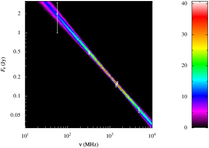
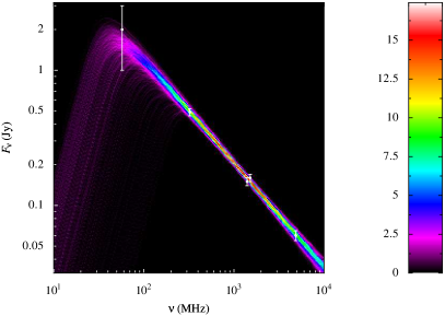
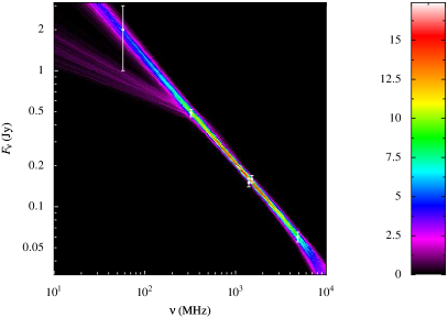
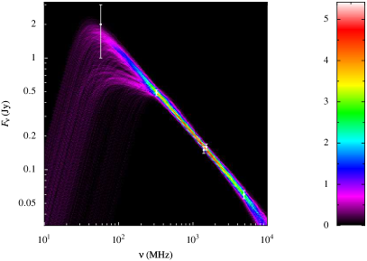
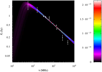
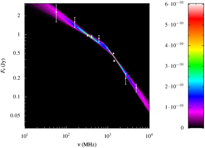
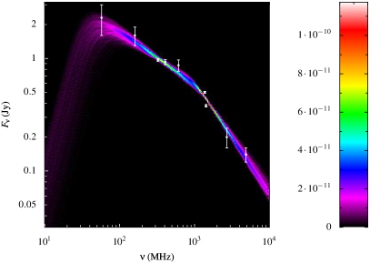
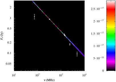
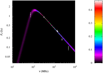
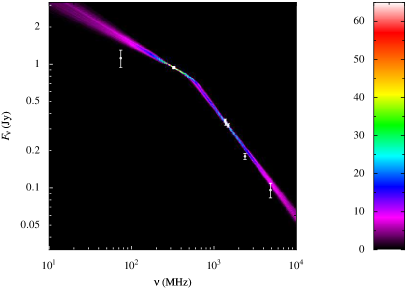
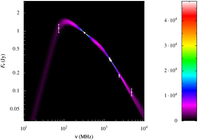
where as before is the hypothesis, i.e., the model for emission and the priors on the model parameters; is the posterior distribution which is an output of the nested sampling; and the integration over is of course over all its dimensions. This probability distribution can then be plotted by assigning frequency to horizontal position, flux density to vertical position and the probability to colour-scale on the plot. Such diagrams are sometimes called fan-diagrams in economics, and I adopt that terminology here. This visualisation approach is shown in Figures 1–3.
3 Implementation
| Power-law (Evidence: 185.874) | Power-law + SSA (Evidence: 76.3034) |
 |
 |
| CI (Evidence: 83.4132) | CI + SSA (Evidence: 27.65) |
 |
 |
| Power-law (Evidence: ) | Power-law + SSA (Evidence: ) |
 |
 |
| CI (Evidence: ) | CI + SSA (Evidence: ) |
 |
 |
| Power-law (Evidence: ) | Power-law + SSA (Evidence: 0.5) |
 |
 |
| CI (Evidence: 70) | CI + SSA (Evidence: ) |
 |
 |
| Overall flux | Spectral index (at frequencies below the break) |
 |
 |
| Frequency of the spectral break | Frequency at which self-absorption becomes important |
 |
 |
The major computational parts of the algorithms described here are implemented in the C++ programming language in two separate libraries:
-
•
bnmin1 This is a minimisation and inference library that contains the nested-sampling algorithms and the supporting functions
-
•
radiospec This is the library specialised for this application, and contains the models of radio spectra and descriptions of observations and their errors
The first of these, bnmin1, is a general purpose minimisation/inference library that may be used in a variety of application. So far I have used this library for phase retrieval holography (Nikolic et al. 2007a, Nikolic et al. 2007b), which is the application for which I first started to develop the library; and for phase correction algorithms for ALMA (Nikolic 2009a and Nikolic 2009b). The library has been available to the public under the GNU General Public License for a number of years and although it has been downloaded occasionally I am not aware of other public work using it. The majority of the functionality described in this paper has only just been added in the release of the library that accompanies this paper. The remaining functionality available in the library includes Levenberg-Marquardt fitting and Markov Chain Monte Carlo (MCMC).
The C++ parts of both of the libraries are relatively self-contained with only two external dependencies: the Boost C++ libraries (Abrahams et al. 2009), and the GNU Scientific Library (Galassi et al. 2009). The build system of bnmin1 is based on the standard AutoTools chain, while radiospec is built using the SCons system.
The top level commands, such as which algorithms to use, to enter the observed data, to control adjustable parameters etc are implemented in the Python programming language. The interface between the C++ libraries and Python is generated automatically using the standard SWIG111http://www.swig.org/ package described by Beazley (2003). This architecture allows easy interactive use of the library. The supporting Python script for this application is available as part of radiospec.
All of the code is available for public download under the GNU General Public License at http://www.mrao.cam.ac.uk/~bn204/galevol/speca/index.html. I should however point out some caveats:
-
•
The packages need to be compiled from source and this typically requires some experience. The instructions posted on the above web-pages will be updated over time to explain how to tackle common problems with compilation that are reported to me
-
•
In order to analyse new observations using existing models, you will need to program in Python. There is no graphical or command shell user interface to this software
-
•
In order to create new models, you will need to program in C++
Included with the code is a script which reproduces the illustrative examples given later in this paper.
3.1 Implementation of radio spectra models
The models of radio spectra are implemented as a polymorphic class hierarchy in C++ in the radiospec package. The base class defining the interface is RadioModel which in turn inherits from the Model class from the BNMin1 package. There are however only two relevant “virtual” functions in the interface:
-
1.
double fnu(double nu) const which computes the flux density at specified frequency nu
-
2.
void AddParams(std::vector< Minim::DParamCtr > &pars) which defines the parameters of the model by adding them to the vector of parameter definitions pars
Any new models with which radiospec is extend must properly define these two functions to be useful.
The reason for adopting the polymorphic inheritance approach rather than the more run-time efficient template approach is that the polymorphic inheritance can be easily accessed and manipulated from Python, allowing for example dynamic composition of several models into a new, more complex, single model.
3.2 Implementation of the likelihood function
The likelihood function for the examples shown here is implemented in the NormalLkl class. This function combines an user specified model (as a pointer to a type RadioModel object), an user specified set of observations (as an object of RadioObs class) and the usual Gaussian probability formula to compute the likelihood.
If a non-Gaussian likelihood function is required, it should be implemented in a similar way to NormalLkl class but it should not be derived from it.
3.3 Implementation of the priors
In the current version of the code, only flat priors which are separable functions of single model parameter are supported. Additionally, every model parameter must have some prior defined for it because this information is used to initialise the nested sampling algorithm. Consequently, the user effectively has to define a parameter-space prior ‘box’ for each problem.
The prior ‘box’ is specified in the Python layer as a dictionary of parameter names that map to a tuple specifying the lower and upper bound of the parameter. An example is given in the file methodex.py.
3.4 Plotting
The plotting of output is implemented using the PyX framework for Python (Lehmann et al. 2009). This library is able to directly write PostScript (PS) and Portable Document Format (PDF) files and to run LaTeX to generate properly type-set labels for the graphs. The main benefits of this library for this application are that it can be used directly from Python and that the output is of high-quality both visually and in terms of the efficiency and readability of the output PostScript code.
The routines that build on top of PyX to make the plots shown in this paper are largely contained in the package PyHLP which is distributed separately from the other packages and can be downloaded at http://www.mrao.cam.ac.uk/~bn204/technotes/pyhlp.html.
4 Results
The data I used to illustrate this approach are taken from Paladino et al. (2009). They are global spectra of three late-type galaxies with measurements at 5 to 7 frequencies in the range 50 MHz–5 GHz. I have taken the measurements and measurement errors listed by Paladino et al. (2009) without any further edits and without referring to the original sources for the archival data that they used.
The spectra of all three galaxies were processed as described above, including the use of the priors listed in Equations 10–13. The results are presented as the fan-plot for each model, together with the evidence value in Figures 1– 3. For NGC 7331, in Figure 4 I also plotted the marginalised distributions of the model parameters.
4.1 NGC 628
The radio spectrum of the galaxy is relatively featureless and can be by-eye seen to be reasonably close to a pure power-law. The analysis presented here also reaches this expected conclusion.
The fan-diagrams of all four models for this object are shown in Figure 1. The combination of model and prior with the highest evidence value is the power-law case, shown in the upper-left panel of this figure. This means that this simple model is the best model for the true underlying process given the observations out of the four models considered here.
The continuous injection model fan-diagram in the lower-left panel shows that it can explain the data in two ways: either the break is at a frequency higher than the highest observations, or, the break is at around 300 MHz and the lowest-frequency data point is predicted with a significant error. Therefore there in principle remains a possibility that this galaxy has a highly aged electron population with an intrinsic injection index of about . This is however unlikely given the lower evidence value of this model compared to the power law.
Finally it can be seen that the absorbed models on the right hand side of Figure 1, i.e., the upper-right and lower-right plots, do not describe the data as well as the non-absorbed models. This is part because the minimum frequency of the turnover was set at 30 MHz by priors.
4.2 NGC 3627
The fan-diagrams for this galaxy are shown in Figure 2. The model with the highest evidence is the continuous-injection model without absorption at low frequencies. The lower evidence of the CI+SSA model indicates that with these data, there is no evidence for absorption in this source.
4.3 NGC 7331
The fan-diagrams for this galaxy are shown in Figure 3. What is noticeable for this galaxy is that the most complex model, the continuous-injection with synchrotron self-absorption model (CI+SSA), has the highest evidence value by several orders of magnitude. This high evidence value implies that this complex model must be preferred given the available data. The fan-diagram of the CI+SSA model, in the lower-right panel of the figure, shows that it reproduces well the observed features of the spectrum while all of the others fail to reproduce one or more features.
The marginalised distributions of the parameters of the CI+SSA model are shown in Figure 4. It shows that the distributions of all of the parameters are well constrained, although at least the spectral index and the break frequency show non-Gaussian distributions. This should be interpreted to mean that care must be taken when using a simple single-value error estimate for these parameters in further calculations.
5 Summary
Fitting of radio spectra of galaxies is a topic that is computationally relatively simple, since most models are either analytic or contain simple one-dimensional integrals. A proper statistical analysis is however not entirely straightforward for a combination of reasons:
-
1.
There are few measurement points (typically 3–10)
-
2.
Errors are often non-Gaussian (e.g., because they are dominated by calibration errors) and are sometimes not well quantified
-
3.
There are many different models that could be tried
An attractive way to tackle this problem is using Bayesian analysis because it provides:
-
1.
A rigorous theoretical framework
-
2.
Objective model selection
-
3.
A natural way to introduce physical constraints on model parameters through priors
-
4.
Full probability distributions for each model parameter
-
5.
A complete picture of any degeneracies in the model parameters
In this paper I have described a publicly available computer code which implements such Bayesian analysis of spectra using the nested sampling algorithm developed by Skilling (2006). This algorithm allows efficient calculation of all of the outputs of Bayesian analysis including the evidence value and the full joint distribution of all parameters. This means analysis is computed quickly and without the need to guide it ‘by hand’, by for example carefully choosing starting positions.
The described code also allows visualisation of how well the each model explains the data using fan-diagrams. I believe this little-used approach to visualisation allows a good and intuitive understanding of implications of a particular distribution of model parameters.
The code described is already being used for several of projects in radio astronomy but I expect it could useful for quite a broad range of applications. Such application to new areas will no doubt lead to discoveries of errors and shortcoming in the code and I would very much appreciate to be notified these at mailto:b.nikolic@mrao.cam.ac.uk. If you obtain useful results from the code without finding any errors or shortcomings, than of course I would be even more happy to hear from you, at the same email address, and can place a link to your paper on the web-pages.
References
- Abrahams et al. (2009) Abrahams D., et al. Boost c++ libraries [online], 2009. Available from: http://www.boost.org/
- Beazley (2003) Beazley D. M., 2003, Future Generation Computer Systems, 19. Available from: http://www.swig.org/
- Feroz & Hobson (2008) Feroz F., Hobson M. P., 2008, MNRAS, 384, 449. arXiv:0704.3704
- Feroz et al. (2009) Feroz F., Hobson M. P., Bridges M., 2009, MNRAS, 398, 1601. arXiv:0809.3437
- Galassi et al. (2009) Galassi M., et al. Gnu scientific library [online], 2009. Available from: http://www.gnu.org/software/gsl/
- Jaynes (2003) Jaynes E. T., 2003, Probability Theory : The Logic of Science. Cambridge University Press
- Kardashev (1962) Kardashev N. S., 1962, Soviet Astronomy, 6, 317
- Lehmann et al. (2009) Lehmann J., Schindler M., Wobst A. Pyx - python graphics package [online], 2009. Available from: http://pyx.sourceforge.net/
- Nikolic (2009a) Nikolic B., 2009a, ArXiv e-prints, ALMA Memo 587. arXiv:0903.1179
- Nikolic (2009b) —, 2009b, ArXiv e-prints, ALMA Memo 588. arXiv:0907.4472
- Nikolic et al. (2007a) Nikolic B., Hills R. E., Richer J. S., 2007a, A&A, 465, 679. arXiv:arXiv:astro-ph/0612241
- Nikolic et al. (2007b) Nikolic B., Prestage R. M., Balser D. S., Chandler C. J., Hills R. E., 2007b, A&A, 465, 685. arXiv:arXiv:astro-ph/0612249
- Pacholczyk (1970) Pacholczyk A. G., 1970, Radio astrophysics. Nonthermal processes in galactic and extragalactic sources, Pacholczyk A. G., ed.
- Paladino et al. (2009) Paladino R., Murgia M., Orrã E., 2009, A&A, 503, 747. arXiv:0905.3643
- Sivia & Skilling (2006) Sivia D. S., Skilling J., 2006, Data Analysis–A Bayesian Tutorial, 2nd edn. Oxford Science Publications
- Skilling (2006) Skilling J., 2006, in ISBA 8th World Meeting on Bayesian Statistics
Publication information
As an experiment, I will be publishing this paper on arXiv only. This is in part because future revision of this paper is likely to be necessary, once the code is used more extensively both by us and hopefully by the general community.
In lieu of the normal referring process, I would be happy to hear from readers on any aspect of the paper and incorporate all corrections and (at least constructive) suggestions in any future versions. All of these will be credited unless requested otherwise. Alternatively if you have more extensive comments I suggest you use the arXiv trackback mechanism.