Probing Backreaction Effects with Supernova Data

Abstract:

As the Einstein equations are non-linear, spatial averaging and temporal evolution do not commute. Therefore, the evolution of the averaged universe is affected by inhomogeneities. It is, however, highly controversial how large these cosmological backreaction effects are. We use the supernova data of the Constitution set up to a redshift of 0.1 in order to analyse to what extent the measurement of the Hubble constant is affected. The size of the effect depends on the size of the volume that is averaged over. The observational results are then compared to the theory of the backreaction mechanism.

1 Introduction

In cosmology it is very common to assume a homogeneous and isotropic universe. As we know that there exist structures in the universe [1], this homogeneity and isotropy can only be statistical on large scales [2], but not exact. Due to the non-linearity of Einstein’s equations spatial averaging and temporal evolution do not commute. Thus, local inhomogeneities can affect the expansion of the background universe via the so-called backreaction mechanism [3, 4, 5, 6]. In this work, we probe the influence of backreaction on the measurement of the Hubble rate using supernova type Ia data.

2 Averaging

Many observables are averaged quantities. As all observed objects lie on our past light cone, it would be appropriate to average the observables over this light cone. This is however a very difficult task that has not been achieved yet. Instead one can use spatial averages at the cost of introducing an error. In order to keep this error at an acceptable level, it is necessary to limit the use of spatial averages to low redshifts. In our analysis we use supernovae up to $z=0.1$. In that range, this averaging method is justified.

The averages of observables are calculated within a certain domain $D$. Its volume is given by

$$V_{D}(t)\equiv\int_{D}W_{D}({\bf x})\sqrt{\mbox{det}g_{ij}}\mbox{d}{\bf x}\;,$$ (1)

where $W_{D}({\bf x})$ is the window function specifying the domain. Then the spatial average of an observable $O$ within $D$ is

$$\langle O\rangle_{D}\equiv\frac{1}{V_{D}(t)}\int_{D}W_{D}({\bf x})O(t,{\bf x})\sqrt{\mbox{det}g_{ij}}\mbox{d}{\bf x}\;.$$ (2)

An effective scale factor $a_{D}$ can be defined via the domain volume:

$$\frac{a_{D}}{a_{D_{0}}}\equiv\left(\frac{V_{D}}{V_{D_{0}}}\right)^{1/3}\;,$$ (3)

where the subscript 0 denotes the present time. The effective Hubble rate then determined by

$$H_{D}\equiv\frac{\dot{a}_{D}}{a_{D}}\;.$$ (4)

Following Buchert’s formalism, the Einstein equations can be averaged in order to obtain the effective Friedmann equations for a dust universe [5]:

$$\left(\frac{\dot{a}_{D}}{a_{D}}\right)^{2} = \frac{8\pi G}{3}\rho_{\rm eff}\;,$$ (5)

$$-\frac{\ddot{a}_{D}}{a_{D}} = \frac{4\pi G}{3}(\rho_{\rm eff}+3p_{\rm eff})\;.$$ (6)

These equation include the energy density and pressure of an effective fluid, which are given by

$$\rho_{\rm eff} \equiv \langle\rho\rangle_{D}-\frac{1}{16\pi G}\left(\langle Q\rangle_{D}+\langle{\cal R}\rangle_{D}\right)\;,$$ (7)

$$p_{\rm eff} \equiv -\frac{1}{16\pi G}\left(\langle Q\rangle_{D}-\frac{1}{3}\langle{\cal R}\rangle_{D}\right)\;.$$ (8)

$\langle Q\rangle_{D}$ denotes the kinematical backreaction and $\langle{\cal R}\rangle_{D}$ the averaged spatial curvature.

We want to analyse the influence of backreaction effects on the measurement of the Hubble rate. Its average value obtained by observing objects within a domain $D$ is denoted as $H_{D}$. Assuming that there exists a global value $H_{0}$, we can define the fluctuation of the Hubble rate as

$$\delta_{H}\equiv\frac{H_{D}-H_{0}}{H_{0}}\;.$$ (9)

Without backreaction the average value $\overline{\delta_{H}}$ equals zero. Considering backreaction effects, the value of $\overline{\delta_{H}}$ becomes slightly negative for small domain sizes. But the main effect is that the variance of $\delta_{H}$ is increased compared to the case when backreaction effects are not taken into account.

3 Gaussian window function

3.1 Method

It is not obvious which choice of window function yields the best results for a test of backreaction effects. The first try was to assume a spherically symmetric domain described by a gaussian window function

$$W_{D}(r)=\frac{1}{\sqrt{2\pi}R_{D}}\exp\left(-\frac{r^{2}}{2R_{D}^{2}}\right)\;,$$ (10)

where $R_{D}$ specifies the size of the domain. Then the variance of $\delta_{H}$ due to backreaction effects is given by [7]:

$${\rm Var}\left(\delta_{H}\right)=\frac{25}{486\pi^{3}}\frac{1}{(1+z)^{2}}\left(\frac{R_{\rm H}}{R_{D}}\right)^{4}\int_{0}^{\infty}\!{\cal P}_{\varphi}(x/R_{D})J^{2}_{3/2}(x){\rm d}x\;,$$ (11)

where $R_{H}$ is the Hubble radius. The values for the power spectrum ${\cal P}_{\varphi}$ are taken from WMAP5 measurements [8].

For the analysis, we use supernova type Ia data from the Constitution set [9] up to a redshift of 0.1. We used the data that were fitted with SALT2 [10]. The number density of SNe needs to be approximately constant within the considered domain. Thus, the number of SNe $N(r)$ in the distance interval $[r,r+{\rm d}r]$ must be proportional to $r^{2}W_{D}(r)$. That means that we have to choose a subset of SNe, whose distribution in space corresponds to that of the considered window function.

(a)

(b)

Figure 1: Gaussian window function. (a) Distribution of the SNe and $r^{2}W_{D}(r)$ for five different values of $R_{D}=45,60,80,100,120$. The black curve is the sum of all five window functions $r^{2}W_{D}(r)$. (b) $\delta_{H}$ obtained from ten different realisations of subsets. Also shown are the variances with and without backreaction.

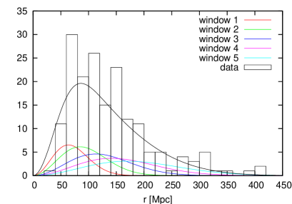
Figure 1a shows the distribution of the 178 SNe in the Constitution set up to redshift 0.1. For the test of backreaction effects, it is essential to compare the value of $\delta_{H}$ of differently sized domains. The domain size can be changed by varying $R_{D}$ as given in equation (10). We chose to use five domains. Their corresponding window functions $r^{2}W_{D}(r)$ are plotted in the figure, the black curve being the sum of these functions. However, the window functions only determine how many SNe at a certain distance are assigned to a subset, but not which individual SNe. The actual assignment of SNe to a subset within one realisation is done randomly, but in a way that all subsets are disjoint and thus statistically independent. As soon as one uses many realisations, i.e. different assignments of SNe to the subsets, the statistical independence is lost.

In order to calculate the Hubble rate $H_{D}$, we need to know the redshift $z$ and the distance modulus $\mu$ for each supernova. The distance modulus, however, depends on the calibration of the absolute magnitude of the SNe. Thus, a different calibration leads to different values of $\delta_{H}$, if one uses a global $H_{0}$ that was not obtained by using the same data set, but by other observations such as WMAP. It turned out that the test result is very sensitive to the calibration. Therefore, we have to determine $H_{0}$ using the same data set as for calculating $H_{D}$.

3.2 Results

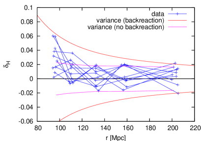
Figure 1b shows $\delta_{H}$ for ten random realisations of subsets. The five data points obtained from the five subsets in each realisation are connected by lines. $r$ is the average distance of the SNe in a subset. The pink curves indicate purely the measurement errors of the SNe. For the red curves $\sqrt{{\rm Var}\left(\delta_{H}\right)}$ from equation (11) is added in quadrature to the measurement errors. Here, the domain scale $R_{D}$ has to be expressed in terms of the average distance as $R_{D}=\sqrt{\pi/8}\,r$. The global Hubble rate that is needed for the calculation of $\delta_{H}$ was chosen such that the data points at large distances lie within the variance limits. There is a trend of increasing $\delta_{H}$ with decreasing distance. The model with backreaction effects seems to describe the data better than the one without these effects.

In order to test backreaction effect, we need however a more quantitative analysis. Therefore, we determined the optimal $H_{0}$ for each realisation once with and once without backreaction effects. Then we calculated the likelihoods of each model given the data. In 27 out of 100 realisations the model including backreaction effects was favoured. However, in none of the realisations one of the two models was favoured significantly.

4 Tophat window function

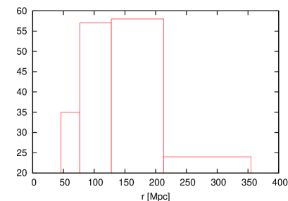
As it was not possible to detect backreaction effects using a gaussian window function, we tried a different ansatz. Since backreaction effects are larger at smaller distances, our aim was to minimize the distance of the first data point. This can be achieved by only using the nearest SNe to calculate the first data point. So we binned the SN data according to distance, where the binwidth is increased with increasing distance (see figure 2a). The corresponding window function is

$$W_{D}(r)=\Theta(R_{D})\Theta\left(r-\frac{5}{3}R_{D}\right)\;.$$ (12)

Then the variance of $\delta_{H}$ is given by

$${\rm Var}\left(\delta_{H}\right)=\frac{2025}{153664\pi^{2}}\frac{1}{(1+z)^{2}}\left(\frac{R_{\rm H}}{R_{D}}\right)^{4}\int_{0}^{\infty}\!{\cal P}_{\varphi}(x/R_{D})J^{2}_{3/2}(x){\rm d}x\;.$$ (13)

The relation between $R_{D}$ and the average distance is $R_{D}=49/68\,r$.

(a)

(b)

Figure 2: Tophat window function. (a) Distribution of SNe. (b) $\delta_{H}$ obtained from the SN subsets. Also shown are the variances with and without backreaction.

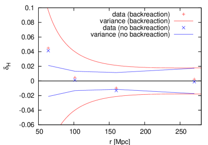
An advantage of the new window function (12) is that the assignment of SNe to subsets is unique. So we do not need to consider different realisations. Like in the previous case, we determined the optimal global Hubble rate $H_{0}$ for the model with and that without backreaction and subsequently calculated $\delta_{H}$ for each subset. The result is shown in figure 2b. Note that the data points for the two models differ slightly as we have used different values of $H_{0}$. The quantitative analysis shows that the model with backreaction is only about twice as likely as the models without backreaction effects. Thus, we have not found any evidence for backreaction.

5 Conclusion

Theoretically, backreaction influences the measurements of the Hubble rate by increasing its variance. This effect should be observed, if it was possible to measure the Hubble rate at different locations in the universe. We are, however, restricted to our local universe. So it is possible that our local measurements are by chance consistent with a model that does not include backreaction effects. If that was the case, we would not be able to detect those effects using the test presented in this work. Therefore, the test can potentially prove the existence of backreaction effects, but it cannot prove that there are no such effects.

Using the currently available supernova data, we could find some slight hint of backreaction, but no evidence. Larger data could help providing that evidence. A larger number of supernovae leads to a smaller variance in the model without backreaction. If the measured values of $\delta_{H}$ stayed approximately the same for a sufficiently large data set, then the data would lie significantly outside the variance limits of a model without backreaction. In that way future data sets have the potential of providing the evidence for the backreaction mechanism.